How will land use affect air temperature in the surface boundary layer? Lessons learned from a comparative study on the energy balance of an oak savanna and annual grassland in California, USA

Abstract

We investigated the effect of land use on differences in air temperature. We based our analysis on a decade of weather and energy flux measurements, collected over two contrasting landscapes, an oak savanna and an annual grassland, growing under the same climate conditions. Over the decade, the daily-averaged, potential air temperature above the aerodynamically rougher and optically darker oak savanna was 0.5°C warmer than that above the aerodynamically smoother and optically brighter annual grassland. However, air temperature differences were seasonal. Smallest differences in potential air temperature occurred towards the end of spring, when much of the soil moisture reservoir was depleted. Largest differences in potential air temperature occurred during the winter rain season when the grass was green and transpiring and when the trees were senescent or deciduous. To understand the effect of land use on the local climate, we examined the concomitant changes in net radiation, sensible and latent heat exchange, the aerodynamic roughness (R_a), the surface resistance to water transfer (R_s), aerodynamic surface temperature and the growth of the planetary boundary layer, with measurements and model computations. Overall, these biophysical variables provide us with mechanistic information to diagnose and predict how changes in air temperature will follow changes in land use or management. In conclusion, land use change is responsible for having a marked impact on the local climate of a region. At the local level, the change in the surface energy balance, towards a darker and rougher surface, will produce an additive increment to climate warming induced by a greater greenhouse gas burden in the atmosphere.

• climate change
• micrometeorology
• energy balance
• savanna
• land use change
• eddy covariance

1. Introduction

Land use change is emerging as one of the major signatures of the new Anthropocene era (Steffen et al., 2007). Across the surface of the planet, land use change is occurring in many different ways and to different extents due to direct and indirect human activities. In the tropics, deforestation is widespread, as land is being cleared for agriculture (DeFries et al., 2002). In temperate zones, afforestation and reforestation are occurring on abandoned agricultural fields, as populations have shifted from farms to cities (Nabuurs, 2004). In semi-arid regions, shrubs are encroaching across many pasture lands (He et al., 2011). Wide regions of deserts and steppes have been transformed into green agricultural landscapes by irrigation (Christy et al., 2006). And across the boreal and western forests of North America accelerated disturbance is occurring through logging, fire (Randerson et al., 2006; Westerling et al., 2006) and insect infestation (Brown et al., 2010).

Land use change plays a critical role in regulating the climate system by changing the Earth's surface radiation balance and the burden of greenhouse gases in its atmosphere (Foley et al., 2005). The consequence of land use change on the land's energy balance is complex because it can modulate fast (hours, days and seasons) biophysical processes in several ways. Specifically, the presence, or absence, of forests affects the energy balance of the land through its modulation of surface properties, such as the surface and planetary albedo, the aerodynamic and surface conductance to heat and moisture transfer and the surface's radiative or aerodynamic temperature (Dickinson, 1983; Verma, 1989; Sellers et al., 1997a; Masson et al., 2003). In principle, albedo is a function of leaf area index, spectral reflectance of the leaves, leaf nitrogen content and the clumping and angle of leaves (Sellers, 1985; Ollinger, 2010). Converting the land from forest to grassland can increase surface albedo by a factor of two (Hollinger et al., 2010). However, the production of reflective cumulus clouds by actively transpiring forests can increase the albedo of that column of air (Bonan, 2008). The aerodynamic conductance is affected by atmospheric stability, the roughness length and the zero plane displacement of the vegetation and wind velocity (Shaw and Pereira, 1982; Verma, 1989). Replacing a forest with grass can decrease the aerodynamic conductance of the surface by factors ranging between two and ten (Kelliher et al., 1993). The surface conductance, or its inverse – the resistance, is most affected by leaf area index, photosynthetic capacity, soil moisture and leaf nitrogen content (Schulze et al., 1994). Replacing a forest with irrigated and fertilised crops can increase the surface conductance by a factor of two (Kelliher et al., 1995; Baldocchi and Xu, 2007). Adjustments in surface temperature caused by trade-offs between latent and sensible heat exchange can have a profound impact on the net radiation balance of the surface – long-wave energy lost by the surface is a function of absolute surface temperature to the fourth power. Warming the surface by 5 K can increase long-wave energy lost to the sky by 7%, according to calculations based on the Stefan–Bolzmann Law (Monteith and Unsworth, 1990). Finally, the depth of the planetary boundary layer is dependent upon sensible heat exchange at the surface (McNaughton and Spriggs, 1986). Hence, one observes deeper boundary layers over forests with higher sensible heat fluxes than shorter vegetation (Barr and Betts, 1997). Together, coupled feedbacks among surface energy balance, the depth of the planetary boundary layer and by the entrainment of air from the free troposphere can alter the air temperature near the land surface by several degrees, Kelvin (McNaughton and Spriggs, 1986; Siqueira et al., 2009).

The goal of this article is to report on the effect of land use on the local climate by comparing the microclimate and energy fluxes that were measured over two contrasting landscapes, an annual grassland and an oak savanna woodland in California. This analysis is based on data acquired over the course of a decade at two field sites that were located 2.6 km away. Hence, they sit on similar soils and experience the same weather. The seasonal aspects of the Mediterranean climate of this region give us the opportunity to compare cases when: (1) the trees were dormant and leafless and the grass was green (autumn and winter); (2) the trees and grasses were both green (spring); and (3) the trees were green and the grasses were dead (summer).

We hypothesise that the air temperature over an oak savanna will be warmer than that above an annual grassland. We formulated this hypothesis on the basis of two, connected lemmas. The first lemma asserts that the savanna is darker than an annual grassland – this feature can cause a savanna to absorb more energy, which in turn can warm the atmosphere more. The second lemma contends that a savanna is aerodynamically rougher – this feature enables the woodland to transfer the extra absorbed energy as sensible heat into the atmosphere more effectively than a grassland, and thereby warming the air more. The seasonal aspects of this landscape allow us to test a set of conditional hypotheses. First, we hypothesise that the annual grassland will experience warmer surface temperatures during the summer when it is senescent. This circumstance will cause it to emit more long-wave energy, thereby reducing its net radiation budget, even more; the grass is dead and highly reflective during the summer. Consequently, the grassland will produce less sensible heat than the savanna and warm the air layer less. Alternatively, we hypothesise that the savanna will produce less sensible heat than the dead grass during the summer less because the transpiring trees will be cooler; this set of linkages will warm the air layer less. Second, we hypothesise that the transpiring grass will be cooler than the dormant and senescent savanna, during the winter, so the grassland will heat the air less. Alternatively, the bare trees, which are not transpiring, but are aerodynamically rough, will convert more available energy into sensible heat and warm the atmosphere more.

We explain the mechanisms, describing our results, through the lens of energy flux measurements and computations based on an energy balance model that is coupled to a one-dimensional planetary boundary layer model (McNaughton and Spriggs, 1986). Specifically, we use the energy flux measurements and model computations to investigate the respective controls by net radiation, albedo, surface temperature, the surface resistance and aerodynamic resistances and depth of the planetary boundary layer on air temperature; this is accomplished by studying how the net radiation budget is modulated and how that energy is partitioned into sensible and latent heat exchange.

2. Materials and methods

2.1. Site information

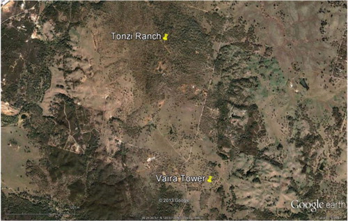
Meteorological conditions and mass and energy fluxes were measured at two field sites, which are located on the lower foothills of the Sierra Nevada Mountains, near Ione, CA (USGS 7.5′ Quadrangle map: Irish Hill). One study site, the Tonzi Ranch, is classified as an oak savanna woodland (latitude: 38.4311°N; longitude: 120.966°W; altitude: 177 m). The second site, the Vaira Ranch, is less than 2.6 km way and is classified as a California, annual grassland (latitude: 38.4133°N; longitude: 120.9508°W; altitude: 129 m); Fig. 1 presents an aerial image of the landscape. Cattle grazed both sites, seasonally, at low stocking rates. Environmental measurements started in early November 2000 at the grassland site and in late April 2001 at the oak woodland; measurements continue as we write this article.

Fig. 1 Image of the field sites under investigation. The Tonzi Ranch is the venue of the oak savanna flux tower. The annual grassland is located on the Vaira Ranch. Both sites are near Ione, CA.

From a micrometeorological perspective, the field sites are nearly ideal. They are on are relatively flat terrain and possess adequate fetch. A uniform fetch of tree/grass savanna extends upwind for about 700 m around a central meteorological tower (Kim et al., 2006). The fetch of the grassland is >100 m; its fetch extends beyond the flux footprint calculated with a two-dimensional model (Hsieh et al., 2000).

Due to the Mediterranean climate of the region, rainfall is concentrated between October and May; essentially no rain occurs during the summer months. Mean annual precipitation is 562 mm, with a standard deviation of 193 mm over the period 1948–2005. Mean daily-averaged air temperature was 15.7±6.8°C.

We quantified the structural features of the oak savanna woodland with a variety of direct and remote sensing methods, including airborne LIDAR, IKONOS and AVIRIS images and ground-based measurements of light transmission (Chen et al., 2006, 2008; Ryu et al., 2010). Blue oak (Quercus douglasii) and grey pine (Pinus sabineana) trees cover about 63% of the landscape. On average, the trees are about 9.4±4.3 m tall and constitute a leaf area index of 0.7.

Leaf area index of the herbaceous vegetation was measured periodically using destructive sampling methods by running samples of leaves through an area meter (LICOR 3100, Lincoln, NE, USA). On average, grass starts growing after the commencement of autumnal rains (after day 300) and starts to senesce shortly after the rains stop in spring (~ day 100) (Ma et al., 2011). The maximum leaf area of the grassland approaches 2 m² m⁻². It occurs near day 80, and results in a closed canopy. In contrast, the herbaceous vegetation in the understory of the savanna is sparser and its maximal leaf area index approaches 1 m² m⁻².

The soil of the grassland site is an Exchequer very rocky silt loam (Lithic xerorthents). The soil of the oak–grass savanna is an Auburn very rocky silt loam (Lithic haploxerepts). Ground-penetrating radar measurements reveal that the soil layer is about 0.60 m thick and that it overlays fractured greenstone bedrock (Raz-Yaseef et al., 2013).

2.2. Meteorological and soil measurements

Solar radiation flux densities were measured above the canopies with an upward and downward facing quantum sensor (PAR Lite, Kipp and Zonen, Delft, The Netherlands), a pyranometer (CM 11, Kipp and Zonen, Delft, The Netherlands), and a net radiometer (NR Lite, Kipp and Zonen, Delft, The Netherlands), respectively. Static pressure was measured with capacitance barometers (model PTB101B, Vaisala, Helsinki, Finland). Rainfall was measured with a tipping bucket rain gauge (TE 5252 mm, Texas Electronics, Dallas, TX, USA).

Air temperature and relative humidity were measured with a platinum-resistance thermometer and solid-state humicap, respectively (model HMP-45A, Vaisala, Helsinki, Finland). These sensors were shielded from the sun and aspirated, yielding an accuracy of ±0.2°C at 20°C. To remove bias errors between two sensors, we referenced the temperature measurements to a standard that was provided by the AmeriFlux project during several site visits (Schmidt et al., 2012); these comparisons occurred at the grassland in 2004 and 2007 and at the savanna in 2005 and 2010. The standard temperature sensor was a shielded, aspirated platinum-resistance thermometer, calibrated against known standards at three points between 0 and 100°C.

Soil moisture was measured using two methods to provide a hybrid measure that assesses the spatial and temporal attributes. Volumetric soil moisture content was measured continuously with an array of frequency domain reflectometry sensors (Theta Probe model ML2-X, Delta-T Devices, Cambridge, UK). The probes sense 60 mm segments of soil and deduce soil moisture by measuring the dielectric constant in the contained soil matrix. Sensors were placed at various depths in the soil (surface, 10, 20 and 50 cm) and were calibrated using the gravimetric method. To augment these temporal measurements with better spatial sampling, we deployed a mini-network of segmented (0–15, 15–30, 30–45 and 45–60 cm), time-domain, reflectometer probes (Moisture Point, model 917, E.S.I Environmental Sensors, Inc, Victoria, British Columbia, Canada). Profiles of soil moisture were sampled every week or two during site visits.

Soil temperatures were measured with multi-level thermocouple probes. The sensors were spaced logarithmically at 0.02, 0.04, 0.08, 0.16 and 0.32 m below the surface. Four probes were placed in the soil at the woodland and two were used to sample soil temperature at the grassland. Soil heat flux density was measured by averaging the output of three soil heat flux plates (model HFP-01, Hukseflux Thermal Sensors, Delft, The Netherlands) at each site. They were buried 0.01 m below the surface and were randomly placed within a few metres of the flux system. The gradual build-up of plant matter changed the thermal properties of the upper layer. Consequently, heat storage was quantified in the upper layer by measuring the time rate of change in temperature using the method of Fuchs and Tanner (1967).

Canopy heat storage of the woodland was calculated by measuring the time rate of change in bole temperature. Bole temperatures were measured in 10 trees using three thermocouples per tree. Those sensors were placed about 0.01 m into the boles and were azimuthally space across a tree at breast height. Using information on tree density and diameter at breast height, the storage measurements of heat flux were scaled to the landscape.

Ancillary meteorological and soil physics data were acquired and logged on Campbell CR-231X and CR-10X data loggers. The sensors were sampled every few seconds and half-hour averages were computed and stored on a computer, to coincide with the flux measurements.

2.3. Eddy covariance instrumentation and flux density calculations

The eddy covariance method was used to measure latent and sensible heat and CO₂ flux densities between the biosphere and atmosphere. Positive flux densities represent mass and energy transfer into the atmosphere and away from the surface and negative values denote the reverse.

Wind velocity and virtual temperature fluctuations were measured with a three-dimensional ultra-sonic anemometer (Windmaster Pro, Gill Instruments, Lymington, UK). CO₂ and water vapour fluctuations were measured with an open-path, infrared absorption gas analyzer (model LI-7500, LICOR, Lincoln, NE, USA). The micrometeorological sensors were sampled and digitised 10 times per second.

At the savanna site, a set of micrometeorological instruments was supported 23 m above the ground (~10 m over the forest) on a walk-up scaffold tower. The gas analyzer was mounted 0.35 m below the sonic and 0.25 m to the side of the anemometer. Another set of flux measurement instrumentation was mounted at 2 m above the ground in the understory. A set of flux measurement instrumentation was also mounted on a tripod tower 2 m above the ground at the grassland. Each tower was protected from the cows with an electrical fence.

In-house software was used to process the measurements into flux densities. The software computed covariances between velocity and scalar fluctuations over half-hour intervals. Turbulent fluctuations were calculated using the Reynolds decomposition technique by taking the difference between instantaneous and mean quantities. Mean velocity and scalar values were determined using 30-min records. The computer program also removes electrical spikes and rotates the coordinate system to force the mean vertical velocity to zero.

The fast response CO₂/water vapour sensors were calibrated every three to four weeks against gas standards. The calibration standards for CO₂ were traceable to those prepared by NOAA's Climate Monitoring and Diagnostic Laboratory. The output of the water vapour channel was referenced to a dew point hygrometer (LI-610, Licor, Lincoln, NE, USA). The calibration zeros and spans have shown negligible drift. Corrections for density fluctuations to CO₂ and water vapour fluctuations were applied to the scalar covariances that were measured with the open-path sensor using theory developed by Webb et al. (1980).

To minimise flux measurement errors, we optimised the experimental setup of the flux covariance using guidance from transfer functions (Moore, 1986); the sampling frequency, sampling height, sensor separation and sensor path length attenuate the flux covariance by <10%. Considering uncertainties with applying the transfer functions – the functional representation of co-spectra vary with canopy height and atmospheric stability (Anderson et al., 1986; Detto et al., 2010) – we chose not to apply them to our data.

This analysis is based on nearly 4000 days of comparative meteorological and energy flux measurements, conducted over a decade. Data gaps were inevitable. We did not fill gaps in meteorological measurements. However, we filled gaps in energy fluxes to compute daily and annual sums of fluxes, with minimal basis. We filled data gaps in the energy fluxes with the mean diel-average method (Falge et al., 2001) and numerical smoothing techniques, which work well for this Mediterranean climate (Ma et al., 2007). The diel means were computed for consecutive 20-day windows to account for seasonal trends in phenology and soil moisture.

One metric of testing the quality of the energy flux density measurements is to test for closure of the surface energy balance (Wilson et al., 2002; Leuning et al., 2012). For these two study sites, energy balance closure was good. For the grassland, the mean of the daily sum of sensible and latent heat exchange (H+λE) (6.43±0.108 MJ m⁻² d⁻¹) was 4.5% greater than the mean of the daily sum of available energy which is composed of net radiation minus storage heat flux (R _n–S) (6.15±0.138 MJ m⁻² d⁻¹). For the oak savanna woodland, the mean of the daily sum of sensible and latent heat exchange (H+λE) (7.85±0.142 MJ m⁻² d⁻¹) was 10% less than the mean of the daily sum of available energy (R _n–S) (8.73±0.173 MJ m⁻² d⁻¹). Part of this energy imbalance was due to bias errors in measuring the canopy heat storage. When we modelled the heat storage of the landscape with a three-dimensional energy balance model, we came to a closer agreement of energy balance (Kobayashi et al., 2012).

2.4. Diagnosing energy flux measurements with the Penman–Monteith equation for latent heat exchange

We inverted the Penman–Monteith equation for latent heat exchange (λE) (Monteith, 1981) to compute the surface conductance, G _sfc, and its inverse, the surface resistance, R _sfc, using field measurements of latent heat exchange (λE), net radiation (R _n), soil heat flux density (S), vapour pressure deficits (D) and the aerodynamic conductance for water vapour transfer (G _a,v=1/R _a,v):1

Other parameters in eq. (1) include the slope of the saturation vapour pressure–temperature curve, (s), air density (ρ), the specific heat of air at constant pressure (C _p) and the psychrometric constant (γ).

We evaluated the aerodynamic resistance to water vapour transfer (R _a,v) as the sum of the resistances for momentum transfer (R _a,m) and the quasi-laminar boundary layer resistance (R _b) (Verma, 1989):2

In eq. (2), u is wind velocity, k is von Karman's constant (0.4), u _* is friction velocity, Sc is the dimensionless Schmidt number and Pr is the Prandtl number.

The aerodynamic surface temperature, T _aero, was computed by inverting the resistance analogue equation for sensible heat exchange, H:3

In eq. (3), G _H is the aerodynamic conductance for heat exchange and was assumed to be equivalent to the aerodynamic conductance for water vapour, G _a,v.

2.5. Coupled surface energy balance-boundary layer growth model

We computed the daily dynamics of surface energy fluxes and the atmospheric state variables, temperature and humidity mixing ratio, by coupling an analytical solution to the surface energy balance (Paw and Gao, 1988) to a one-dimensional, clear-sky planetary boundary layer model (McNaughton and Spriggs, 1986). We summarise the key attributes of the model next. Details of the energy balance computations are given in Appendices A1 and A2.

The model considers the exchange of heat and moisture in and out of the top and bottom of a column of air that is capped by the planetary boundary layer. The time rate of change of potential temperature (θ _m) in the mixed layer is a function of the height of the mixed layer, h, its time rate of change, dh/dt, sensible heat flux at the land surface, H, and the entrainment of warm air (θ _e) as the mixed layer grows and entrains air from the inversion above the mixed layer:4

The subscript ‘m’ refers to the mixed layer and the subscript ‘e’ refers to the air mass above the entrainment layer. Similarly, we can express the time rate of change of the mixing ratio of water vapour, q _m, in the mixed layer as:5

Here, the surface flux is defined by the evaporative flux density, E, and q _e is the mixing ratio of vapour above the entrainment layer. The additional unknown is the time rate of change of the height of the mixed layer, dh/dt. A simple but robust scheme for computing dh/dt is:6

In eq. (6), H _v is the virtual temperature heat flux, which is defined in terms of sensible and latent heat flux densities:7

is the virtual temperature inversion strength. It is a function of the slopes of the inversions associated with potential temperature and specific humidity:8

3. Results and discussion

3.1. Where was it warmer?

To answer the overarching question, ‘where was it warmer?’ we compared 10 years of diel-averaged measurements of potential air temperature over the two contrasting ecosystems; we used potential temperature to compensate for differences in measurement height (Arya, 1988). Figure 2a shows a one-to-one plot between potential air temperatures measured above the grassland (y) and the oak savanna (x). Fitting a linear regression on 3771 daily-mean samples yielded a slope equal to 1.007, a zero intercept equal to −0.684 and r ² equal to 0.988. In summary, these air temperatures were highly correlated with one another, but the negative intercept indicates that the potential air temperature was notably warmer over the oak savanna, compared to the annual grassland.

Fig. 2 A comparison in daily-averaged potential air temperature an annual grassland and savanna ecosystem. These data were acquired between 2001 and 2011. (a) one–one plot between measurements made over the oak woodland and the annual grassland; (b) probability density function (pdf) of potential temperature differences measured over the woodland and grassland. The probability density function, defined by kernel smoothing method, a non-parametric technique, is superimposed upon the histogram.

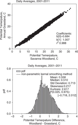
To investigate these data with greater statistical rigor, we examined the distribution of the probability densities of the paired differences in daily-mean, potential air temperature for the savanna, or oak woodland, and the annual grassland, θ _a(savanna)−θ _a(grass) (Fig. 2b). The mean paired temperature difference was 0.558°C, on a standard deviation of ±0.713°C. We also determined that the probability distribution was non-Gaussian, as the median was 0.510°C, the skewness was 0.217, the kurtosis was 2.617, and the 95% confidence interval of the probability distribution ranged between −0.7184 and 2.012°C.

Because the probability distribution of data was non-normal, we applied non-parametric statistics to test if the difference in the paired potential air temperature measurements was significantly different from zero. We computed the 95% confidence interval about the median using the method of McGill et al. (1978); it was computed to be ±0.0807. Based on these statistical metrics, we conclude that the median of the paired potential air temperature differences (0.510°C) was significantly different than the null hypothesis that the median of the potential air temperature differences was equal to zero, at the 5% level of significance (p=0.05). In summary, mean daily potential air temperature above the oak savanna woodland was warmer than the mean daily potential air temperature above the grassland over the course of a decade. However, the probability distribution tells us there were many episodes when the potential air temperature above the grassland was warmer than over savanna.

3.2. When was it warmer?

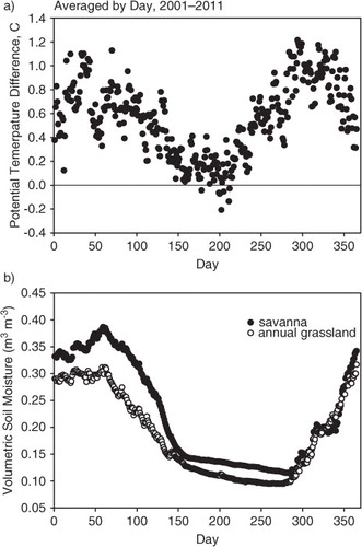
Because of seasonal changes in structure and function of the two ecosystems, as well as changes in soil moisture, solar radiation and other weather variables, it is pertinent to investigate how the mean differences in potential air temperature varied with day of the year and time of the day. Figure 3a shows the seasonal course in the mean difference between potential air temperature at the oak savanna and annual grassland sites; the data were binned by day and averaged by years. Figure 3b shows the corresponding soil moisture for the mean annual cycle. We observed considerable seasonal variation in potential air temperature differences. The greatest temperature differences, ranged between 0.4 and 1.2°C, and occurred during the winter period (days 1–80); this period corresponded to when the trees were dormant, the grass was green and transpiring and soil moisture was greatest. A decline in potential air temperature differences started in the spring after the trees began transpiring (after day 80). This decline in potential air temperature differences continued through the period of rapid soil moisture extraction, to about day 150. The smallest temperature differences occurred during the spring/summer transition, between days 150 and 220, when soil moisture was low (<0.15 m³ m⁻³), the grass was dying and the trees were green and transpiring at moderate rates; during this period, differences in potential air temperature ranged between 0.2 and −0.2°C. Later in the summer (after day 220), the potential air temperature differences increased with time, as the trees closed their stomata further, due to chronic soil moisture deficits; this increase in potential air temperature differences lasted until the start of the autumn rain period and leaf senescence (after day 270).

Fig. 3 (a) Seasonal course in diel-averaged potential temperature between an oak savanna and an annual grassland ecosystem. (b) Seasonal course in volumetric soil moisture. The data were bin-averaged by day for the period 2001–2011.

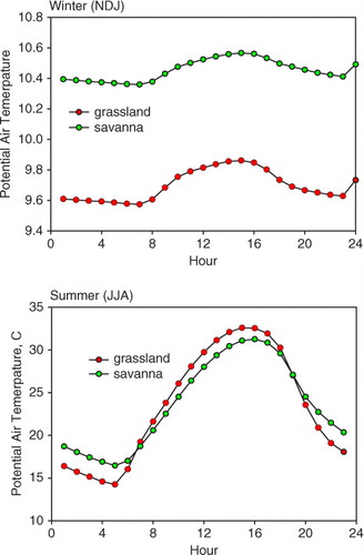
With regards to time of day, we find that the potential air temperature differences depended upon season (Fig. 4). During the winter, dormant period (November–December–January), the potential air temperature over the oak savanna was 0.76°C warmer, on average, than the grassland during both the day and night. During the summer period (June–July–August), potential air temperature above the savanna was 2.2°C warmer than that above the grassland during the night and the air above the grassland was up to 1.7°C warmer than the air above savanna during the day.

Fig. 4 Mean diurnal plot of air temperature over an oak savanna and an annual grassland. These data were binned by hour and were averaged over multiple years. (a) dormant period months, November–December–January, N–D–J; (b) summer (June–July–August, J–J–A).

3.3. Why were there seasonal variations in potential air temperature differences?

To diagnose and explain the mechanisms causing the seasonal variation in potential air temperature differences, we inspect the energy fluxes and the associated aerodynamic and surface resistances that were measured over the two canopies, next.

Over the course of the year, the oak savanna converted more incoming short- and long-wave energy from the sun and sky into net radiation than the grassland (Fig. 5). The mean annually integrated difference in net radiation between the savanna and grassland, averaged over the decade, was 0.849 GJ m⁻² y⁻¹ (Table 1). The mean diel difference in R _net, averaged over a decade, was 2.32±0.122 (95% CI) MJ m⁻² d⁻¹ (Table 2). On a seasonal basis, this difference in net radiation exceeded 5 MJ m⁻² d⁻¹ during the summer; this difference diminished during the spring; and, autumn and net radiation flux density values overlapped one another during the winter. The upper bound of albedo for the grassland approached 0.30 during the summer, and its lower bound approached 0.15 during the winter period (Hollinger et al., 2010). We did not have independent measurements of albedo from the woodland, but a synthesis of measurements across broad-leaved deciduous forests in the Ameriflux network shows albedo was about 0.15 (Hollinger et al., 2010).

Fig. 5 Yearly course in daily-integrated net radiation flux density, averaged by day for the period 2001–2011, for a grassland and savanna ecosystem.

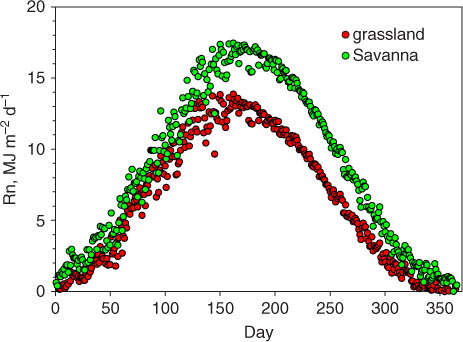
Table 1. Mean annual sums of energy flux densities and mean annual average of potential air temperatures

Variable	Unit	Annual grassland	Oak savanna
R net	GJ m^−2 y^−1	2.326	3.175
H	GJ m^−2 y^−1	1.574	1.993
LE	GJ m^−2 y^−1	0.844	1.260
G	GJ m^−2 y^−1	0.0393	0.0081
θ pot	°C	15.56	16.16

Table 2. Comparison in mean differences in daily-integrated energy fluxes and average potential temperature over an oak savanna and annual grassland

	Units	Mean difference: woodland – grass	95% CI
R net	MJ m^−2 d^−1	2.32	±0.122
H	MJ m^−2 d^−1	0.667	±0.050
λE	MJ m^−2 d^−1	0.6283	±0.046
θ pot	°C	0.558	±0.0228

Note: Statistics on the 95% confidence interval is given on 3770 degrees of freedom.

We note that the summer period, with the greatest differences in net radiation, corresponded with the period with the smallest differences in potential air temperature (days 150–220). Also, we note that the winter period with the least differences in net radiation (days 1–80) corresponded with the period with the greatest differences in potential air temperature. Hence, differences in net radiation balance, alone, were not sufficient to explain the potential air temperature differences observed above these two contrasting plant canopies.

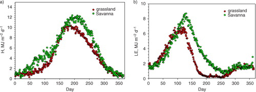
Over the course of a year, the excess net radiation at the oak savanna yielded greater sensible heat flux into the atmosphere, compared to the grassland (Fig. 6a). On an annual basis, the oak savanna injected 0.419 GJ m⁻² y⁻¹ more sensible heat into the atmosphere than the grassland (Table 1). Sensible heat flux density differences were greatest during the winter (0.92 MJ m⁻² d⁻¹), when the trees were leafless and the grass was green, and during summer and early autumn (1.25 MJ m⁻² d⁻¹), when the trees were green and transpiring and the grass was dead. During the spring and autumn, sensible heat flux densities, measured over the two contrasting landscapes, were similar.

Fig. 6 (a) Yearly course in daily-integrated sensible heat flux density (H), averaged by day for the period 2001–2011, for a grassland and savanna ecosystem. (b) Yearly course in daily-integrated latent heat flux density (LE), averaged by day for the period 2001–2011, for a grassland and savanna ecosystem.

Ironically, the periods with the greatest and least temperature differences corresponded with periods when the differences in sensible heat exchange were greatest. Therefore, seasonal differences in sensible heat exchange do not produce satisfactory explanations for the seasonal differences in potential air temperature either.

Only part of the excess net radiation, absorbed by the oak savanna during the summer, was consumed as sensible heat exchange. The other part of excess energy was consumed by latent heat exchange (Fig. 6b), which on an annual basis was favoured over by savanna by 0.416 GJ m⁻² y⁻¹. Conversely, differences in latent heat exchanges changed with the seasons. During the winter, latent heat exchange by the green grass was slightly greater (0.52 MJ m⁻² d⁻¹) than that from the dormant and deciduous oak savanna, with a grass understory. During the spring/summer transition period, latent heat exchange over the savanna was much greater (2.7 MJ m⁻² d⁻¹) than that measured over the senescing grass.

Small differences in latent heat exchange, during the winter, did not generate large enough differences in evaporative cooling to offset the differences in sensible heat exchange, thereby yielding the greatest potential air temperature differences then. The extra evaporative cooling achieved by the oak savanna woodland during the spring/summer transition was partly responsible for the reduction in potential air temperature differences that were observed then, despite the additional net radiation that was available to the savanna. However, as we will show below, differences in latent heat exchange do not provide the full explanation for the observed temperature differences, either.

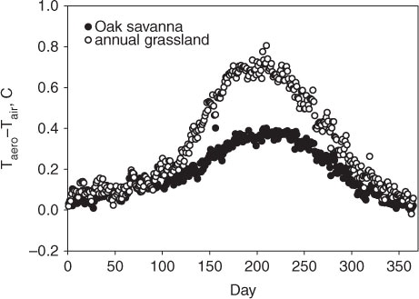
Surface temperature provides one node of the energy potential that drives sensible heat into the atmosphere. The temperature gradient between the aerodynamic surface (eq. 3) and the air above varied with location and time of year (Fig. 7). In general, the grassland maintained a stronger surface-air temperature gradient than the savanna. The greatest temperature gradient approached 0.8°C and occurred during the summer when the grass was dead. In contrast, temperature gradients were less than 0.15°C when the grass was green and transpiring.

Fig. 7 Yearly course in the daily-average difference between the aerodynamic surface temperature, as computed from the surface energy balance, and air temperature.

Despite the fact that the grassland surface temperature was warmer than the savanna, the savanna was able to inject more sensible heat into the atmosphere because it was aerodynamically rougher than the grassland (Fig. 8a); in general, the aerodynamic resistance of the oak savanna woodland was about one-half of that of the grassland.

Fig. 8 (a) Yearly course in daily-averaged aerodynamic resistance (R _a), averaged by day for the period 2001–2011, for a grassland and savanna ecosystem. (b) Yearly course in daily-average surface resistance (R _sfc), averaged by day for the period 2001–2011, for a grassland and savanna ecosystem.

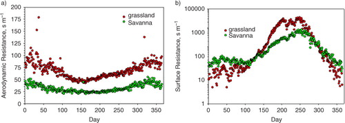
Finally, we inspect the surface resistance, R _sfc, by inverting the Penman–Monteith equation (eq. 1); it gives us information on how the differences between leaf area index and soil moisture impact stomatal conductance, which in turn governs the partitioning of available energy into sensible and latent heat exchange. Fig. 8b shows that the grass possessed a lower surface resistance (<100 s m⁻¹) than the savanna (it ranged between 100 and 200 s m⁻¹), during the winter (days 1–80), as the grass was green and transpiring, while the leafless and dormant trees stood over a green grass understory. During the summer, the surface resistance of the grassland was huge (>10 000 s m⁻¹) due to the dead state of the grass and the extremely dry state of the soil; volumetric water content was less than 0.05 m³ m⁻³. In contrast, the two ecosystems experienced similar surface resistances during the spring and during the autumn, after the first rains occurred and wetted the region again (after day 270).

In relation to surface resistances, we observed the smallest potential air temperature differences during the summer when the surface resistances differed by a factor of 10. Hence, this biophysical factor does not provide the clue explaining these temperature differences, either. However, warmer air temperatures over the savanna, during the winter, are consistent with the fact that its surface resistance was more than double that experienced by the greener grassland.

At this stage we can draw a set of summary statements. The greatest differences in potential air temperature occurred during the winter when net radiation fluxes overlapped one another, more sensible heat exchange was lost by the savanna, and more latent heat was lost by the grass. These differences in how energy was partition occurred because the grass maintained a lower surface resistance, while the woodland established a smaller aerodynamic resistance, thereby enabling the woodland to inject more sensible heat into the atmosphere and warm the air more.

We observed the smallest differences in potential air temperature during the spring/summer transition despite the fact that the savanna gained much more net radiation and lost much more sensible heat, and, despite the fact that the surface temperature of the grassland was warmer than that of the savanna. Greater latent heat exchange by the savanna and more long-wave energy lost by the grassland diminished the potential air temperature differences between the two sites. Yet, a complete explanation for these temperature differences remains unresolved with our measurements, alone. To complete our analysis, we apply a coupled energy balance/planetary boundary layer model to this problem.

3.4. Diagnosing our measurements with a coupled energy balance/planetary boundary layer model

Inspection of the surface energy balance informs us that land use change will alter the aerodynamic roughness (R _a), the surface resistance (R _s), surface's radiative temperature (T _sfc), long-wave energy loss (L↑), and the net radiation balance (R _n). It will also change the depth of the planetary boundary layer, which has the potential to buffer increases in air temperature against incremental changes in sensible heat exchange.

It is difficult to conduct manipulative experiments that alter all these factors in a systematic way across a spectrum of surface conditions. Instead, biophysical models can play a pivotal role in diagnosing the theoretical effects of altering these biophysical variables on the local climate. In this section, we use model computations to help us explain interactions acting on the field data that were reported above. In particular, they help us to understand the role of variables that we cannot measure well or at both sites, like albedo, radiative surface temperature and growth of the planetary boundary layer (z _i ).

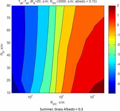
In the first case, we reference computations of air temperature and energy exchange to the conditions of the savanna experienced during the spring/summer transition (days 150–220), yielding an albedo of 0.15, a surface resistance (R _sfc) of 2000 s m⁻¹, and an aerodynamic resistance (R _a) of 20 s m⁻¹. Simulations assumed a clear day with a sinusoidal variation in solar radiation that reached a maximum value of 1000 W m⁻². Also, we assumed that initial air temperature was 20°C, based on data in Fig. 4.

Figure 9 compares temperature differences, referenced to the condition representative of the savanna, to changes in the aerodynamic and surface resistances. As R _a increases from 10 to 80 s m⁻¹ and R _sfc increases from 20 to 20000 s m⁻¹, one sees that air temperature differences, range from being 7°C cooler than the savanna-like conditions to being 2°C warmer. If we focus on the set of conditions that evoke the grassland, during the spring/summer transition (R _a>60 s m⁻¹; R _sfc>10000 s m⁻¹), we calculate that air temperature is between 0 and 1°C warmer than the savanna-like conditions. These values are consistent with the observations reported in Figs. 3 and 4.

Fig. 9 Model computations of air temperature, referenced to temperatures above conditions experienced by the savanna (R _a=20 s m⁻¹; R _sfc=200 s m⁻¹; albedo=0.15), for summer-like weather. The model was run for a range of values in the aerodynamic and surface resistances. We assumed the albedo of the grass was 0.3.

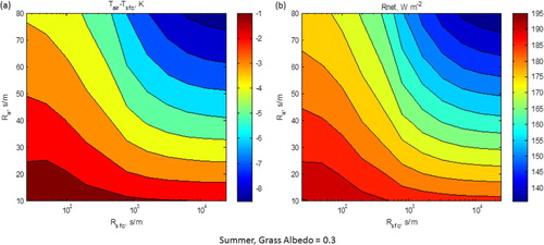
Theoretical air temperatures for the biophysical conditions experienced by the grassland hovered close to the oak savanna for two reasons. First, the dead grass, with a large surface resistance produced radiative surface temperatures up to 8°C warmer than the air temperature (Fig. 10a); this produced a larger loss of long-wave energy, which is a function of surface temperature to the fourth power. Higher flux densities of out-going long-wave energy, combined with a highly reflective surface, yielded a net radiation balance that was 40–50 W m⁻² less than for the conditions experienced by the savanna (Fig. 10b).

Fig. 10 (a) Model computations of air minus radiative surface temperatures, as a function of aerodynamic and surface resistances. (b) Model computations of net radiation, as a function of aerodynamic and surface resistances. Computations assumed albedo equalled 0.3 and summer time conditions of temperature and sunlight.

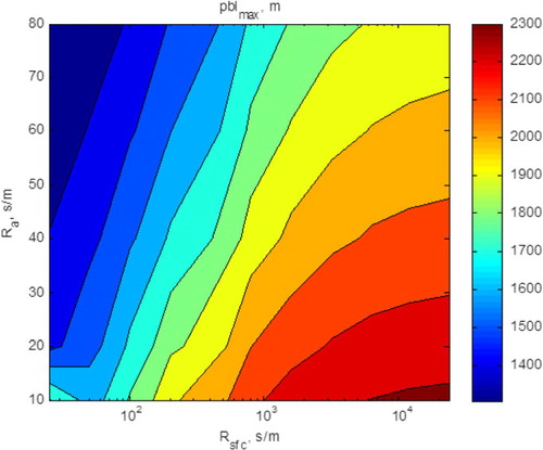
In the end, the extra energy injected into the atmosphere over the savanna-like conditions did not lead to large air temperature differences, because large flux densities of sensible heat promoted deep growth in the planetary boundary layer (Fig. 11); for the meteorological and biophysical conditions experienced by the savanna and grassland during the spring/summer transition, the depth of the planetary boundary layer could reach over 2000 m. While the planetary boundary layer model was simple and one-dimensional, its depth was consistent with measurements by Bianco et al. (2011), who studied the seasonality of boundary layer growth in the nearby Central Valley.

Fig. 11 Three-dimensional plot between maximum growth of the planetary boundary layer as a function of the aerodynamic and surface resistances. Computations were performed for summertime meteorological conditions and the biophysical conditions of the annual grass.

The second model case study is for the winter period when the grass was green and the trees were deciduous, over a green grass understory, yielding a surface resistance (R _sfc) of 200 s m⁻¹ and an aerodynamic resistance (R _a) of 20 s m⁻¹. These simulations assumed a clear day with a sinusoidal variation in solar radiation that reached a maximum value equal to 500 W m⁻². We also assumed that initial air temperature equalled 10°C, based on Fig. 4.

Figure 12 shows how air temperature differences, against the savanna-like reference case, varied with R _a and R _sfc. In this situation, we focus on temperature differences for the region where R _sfc is <200 s m⁻¹ and R _a is >60 s m⁻¹, which typified the grassland during the winter (Fig. 8a and b). Under this combination of conditions, we find that the air temperature above the savanna-like surface was 1–2°C warmer than the range of conditions experienced by the biophysical conditions that were indicative of the grassland. Again, these computations are broadly consistent with the observations reported in Figs. 3 and 4.

Fig. 12 Model computations of air temperature, referenced to temperatures above conditions experienced by the savanna (R _a=20 s m⁻¹; R _sfc=200 s m⁻¹; albedo=0.15), for winter-like meteorological conditions. The model was run for a range of values in the aerodynamic and surface resistances. We assumed the albedo of the grass was 0.15.

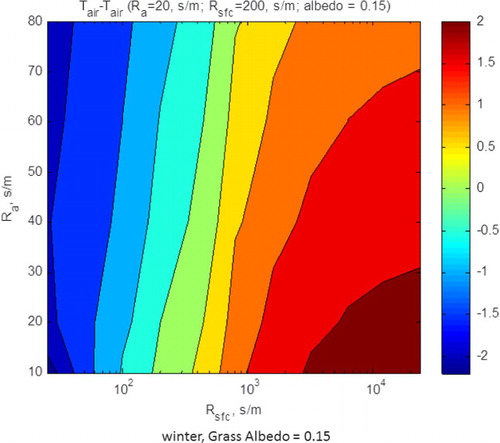
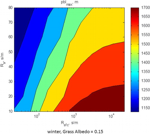
Under winter conditions, there are much smaller differences between surface and air temperatures, yielding smaller differenced in outgoing long-wave radiation and similar values of net radiation (not shown). Yet, greater differences air temperature above the biophysical conditions representative of the grass and savanna are able to evolve, theoretically, because the depth of the winter planetary boundary layer is much less (1000–1500 m, Fig. 13) than under summer-time conditions (2000–2500 m, Fig. 11).

Fig. 13 Three-dimensional plot between maximum growth of the planetary boundary layer, shown as a function of the aerodynamic and surface resistances. Computations were performed for winter-time meteorological conditions and the biophysical conditions of the annual grass.

3.5. The role of this study, in conjunction with the literature

In general, the results from this study are consistent with the findings from Lee et al. (2011), who examined air temperature over a network of forest sites in North America and compared their temperatures with those in nearby clearings; air temperatures over forested lands across North America are reported to be 0.85±0.44°C warmer than nearby open landscapes. However, the gross and net effects of land use change on the energy exchange at regional scales are complex, conditional, and in some instances counter-intuitive and controversial – in some regions land use change can cause regional-scale warming, and other regions it can lead to cooling. In the boreal zone, for example, the presence of forests darkens the snow covered surface during the winter, warming the surface air, compared to snow covered fens and bogs (Sellers et al., 1997b). At the interface between the Boreal and Arctic zones, the expansion of the tree line can darken the albedo of the present tundra and provide a new source of water vapour to the atmosphere through enhanced transpiration (Swann et al., 2010). In the tropics, trees facilitate the transfer of moisture from the soil, forming clouds and increase the planetary albedo (Bonan, 2008). This set of feedbacks cools the surface occupied by forests compared to land replaced by pastures (Jackson et al., 2008; Anderson et al., 2011; Lee et al., 2011). Furthermore, replacing C₃ tropical trees with C₄ grasses amplifies the reduction in surface conductance and increases the potential warming effect on the climate (Bounoua et al., 2002, 2006). The replacement of semi-arid woodlands with grass and shrubs yields some counter-intuitive findings on mass and energy exchange, worth discussing. Woody vegetation is darker than surrounding shrub and grasslands, causing savannas and pine forests to absorb much more solar energy (Montes-Helu et al., 2009; Rotenberg and Yakir, 2011). But more effective convective heat loss and evaporative cooling cause aerodynamically rough forests to experience lower surface temperatures than contrasting smoother landscapes. In one instance, the surface temperature of a transpiring forest plantation in a desert region was 5°C cooler than the surrounding landscape (Rotenberg and Yakir, 2010).

Paired micrometeorological studies sometimes receive criticism about being subject to pseudo-replication because they are un-replicated, per se (Hurlbert, 1984). Yet, comparative ecosystem studies can provide novel information ecosystem–climate–atmosphere interactions (Carpenter et al., 1995). Specifically, comparative studies on the mass and energy exchange of sites differing in land use can serve as field laboratories for studying and understanding the effect of forestation and deforestation. Despite the power of this approach, relatively few paired studies have addressed the roles of the presence/absence of forests on surface energy fluxes using comparative studies (Denmead, 1969; Eugster et al., 2000; Baldocchi et al., 2004; Juang et al., 2007; Rotenberg and Yakir, 2010). More often, scientists have tracked the effects of land use change on energy exchange using measurements across broad ecological gradients that may experience different weather and soils (Baldocchi et al., 2000; Lee et al., 2011; Krishnan et al., 2012) or across a chronosequence following disturbance (Amiro et al., 2006; Goulden et al., 2006).

In recent years, there has been a growing body of literature defending large-scale studies (Carpenter et al., 1995; Oksanen, 2001; Schank and Koehnle, 2009). Oksanen (2001), for example, concludes that ‘The concept pseudo-replication amounts to entirely unwarranted stigmatization of a reasonable way to test predictions referring to large-scale systems’. Here, we studied the short- and long-term temperature dynamics of two contrasting ecosystems, many hundred hectares in area (Hsieh et al., 2000; Schmid, 2002). Because our measurements sampled a large footprint, we were able to measure the state of the general population, rather than deducing its expected value statistically with a replicated set of small and infrequent samples. We contend that repeated temporal sampling of meteorological variables is not pseudo-replication, as suggested by Hurlbert (1984), for two reasons. First, the theory of ergodicity tells us we can substitute spatial sampling with temporal sampling (Panofsky and Dutton, 1984). And, second, we found that successive temporal measurements were not auto-correlated; the sub-hourly temperature measurements were uncorrelated after 12 h and the daily-averaged data became uncorrelated after 90 days. Consequently, we collected a large number of independent statistical samples of temperature at the two contrasting field sites that were representative of large areas. We also contend that repeated temporal sampling reduces the sampling error and increases the precision in detecting differences between two treatments (Moncrieff et al., 1996).

4. Conclusions

Using an extensive decade-long dataset of meteorological conditions, we show that changes in land cover have a marked impact on the air temperature of a landscape. Specifically, we observed that the potential air temperature over an oak savanna was 0.5°C warmer than the air above an annual grassland, 2 km away.

Using a combination of energy flux measurements and model computations with a coupled energy balance/planetary boundary layer model, our data support the overarching hypothesis that the air above the oak woodland is warmer than that above the grassland in part because the oak woodland is darker, so it absorbs more radiation. Furthermore, the oak woodland is aerodynamically rougher. Consequently, is able to inject more sensible heat into the atmosphere than the grassland. But, this extra sensible heat did not convert into warming linearly. The magnitude of the temperature differences above the savanna and grassland was conditional on time of year, phenology, biophysical conditions of the surface and the depth of the planetary boundary layer.

The greatest differences in potential air temperature occurred during the winter when net radiation fluxes overlapped one another, more sensible heat exchange was lost by the savanna, and more latent heat was lost by the grass. These differences in how energy was partition occurred because the grass maintained a lower surface resistance, while the woodland established a smaller aerodynamic resistance, thereby enabling the woodland to inject more sensible heat into the atmosphere and warm the air more. During the winter, the planetary boundary layer did not grow deep, so differences in sensible heat could translate into relatively large differences in air temperature.

We observed the smallest differences in potential air temperature during the spring/summer transition despite the fact that the savanna gained much more net radiation and lost much more sensible heat, and, despite the fact that the surface temperature of the grassland was warmer than that of the savanna. Greater latent heat exchange by the savanna and more long-wave energy lost by the grassland diminished the potential air temperature differences between the two sites. Yet, a complete explanation for these temperature differences depended upon computations of the growth of the planetary boundary layer. During the summer, the planetary boundary layer could grow up to 2500 m and buffer the daily range of air temperature.

In closing, land managers are faced with a number of interesting and conflicting ecological services regarding the presence or absence of forests, as a factor for mitigating climate change. These ecosystems are effective carbon sinks and provide a wide range of favourable ecosystem services outside climate regulation like habitat, soil preservation and water storage. But, forests are also darker, so they can absorb more energy. And, forests may transpire more than grass, causing their surface temperatures to be cooler through latent heat exchange. And forests are aerodynamically rougher than grasslands, so they are able to exchange sensible heat more effectively across a smaller temperature gradient, than grasslands. Consequently, forests may recharge less groundwater than other vegetation classes (Kim and Jackson, 2012) and provide less run-off for stream flow (Marc and Robinson, 2007) compared to grasslands.

Acknowledgements

This research was supported by the US Department of Energy Terrestrial Carbon Program, grant No. DE-FG03-00ER63013 and DE-SC0005130 and the University of California Agricultural Experiment Station. The authors thank Joe Verfaillie and Ted Hehn for their technical help; they have been instrumental in ensuring that the operation of this flux system runs continuously and is of the highest quality. Work on this topic was catalysed by a National Center for Ecological Analysis and Synthesis (NCEAS) workshop, organised by Jim Randerson and Rob Jackson. They thank Dr. Naama Raz-Yassef for providing an internal review. Finally, they thank the Tonzi and Vaira families for access to their ranches for our research.

7. Appendix

A.1. Details on the energy balance and surface temperature computations

To solve for sensible and latent heat exchange in the coupled energy balance/boundary layer model, we relied on a solution to the quadratic equation for latent heat exchange (λE; W m⁻²) (Paw and Gao, 1988):A1

The coefficients for the quadratic equation for λE are as follows:A2 A3 A4

We also employed a solution to the quadratic equation, defining the difference between surface and air temperature (ΔT), was derived from the leaf energy balance relationship so an analytical solution could be used to compute leaf temperature (Paw, 1987):A5

These coefficients are defined as follows:A6 A7 A8

Other variable in eqs. (A1–A7) are defined as follows: ɛ is emissivity, σ is the Stefan–Boltzman constant, ρ _a is air density, λ is the latent heat of vaporisation, T _k is absolute temperature (K), G _w is the conductance for water transfer (it combines the surface conductance, G _s, and the aerodynamic conductance for vapour transfer, G _a,v, in parallel; m s⁻¹), G _h is the aerodynamic conductance for sensible heat transfer (m s⁻¹), C _p is the specific heat of air, Q is absorbed energy (incoming short- and long-wave radiation, minus reflected short-wave radiation; W m⁻²), S is soil heat flux density, m _v and m _a are the molecular weights of vapour and dry air (g mol⁻¹), P is pressure (kPa), e _s is saturated vapour pressure (kPa) and e _a is the ambient vapour pressure (kPa).

Table A1. List of initial conditions and parameter values used to evaluate the coupled surface energy balance/boundary layer model

	R gmax	Air temperature, t=0	Humidity	Albedo, grass	Albedo, savanna	R sfc, grass	R sfc, savanna
Summer	1000 W m^−2	20°C	1.5 kPa	0.20	0.15	25 s m^−1	200 s m^−1
Winter	500 W m^−2	10°C	1.0 kPa	0.40	0.15	10000 s m^−1	3000 s m^−1

R _gmax is the value of solar radiation at mid-day. R _sfc is the surface resistance.

A.2. Details on the fluxes and state variables using the coupled surface layer-planetary boundary layer model computations

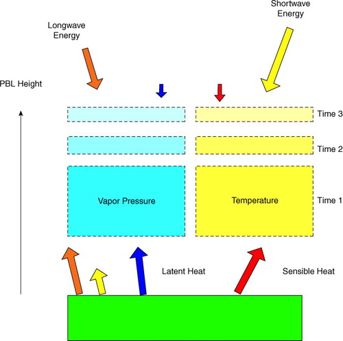
The coupled surface layer-planetary boundary layer model was used to compute surface and entrainment fluxes of latent and sensible heat, and in turn these were used to compute the state of temperature and humidity in the mixed layer and the incremental growth of the mixed layer (Fig. A1). The model was evaluated at hourly time steps. Prescribed initial meteorological conditions are listed in Table A1. Energy fluxes and meteorological conditions were computed for ideal, clear sky conditions, representative of winter and summer days. We assumed that the hourly time course of solar radiation followed a half-sine pattern, symmetric about a mid-day maximum. The initial depth of the planetary boundary layer was assumed to be 100 m and wind velocity was held at 3 m s⁻¹.

Fig. A1 Schematic of the coupled surface energy balance and planetary boundary layer model. The model identifies the energy fluxes at the lower and upper boundaries of the planetary boundary layer and how the layer grows with each time step.

References

- Amiro B. D , Barr A. G , Black T. A , Iwashita H , Kljun N , co-authors . Carbon, energy and water fluxes at mature and disturbed forest sites, Saskatchewan, Canada. Agri. Forest Meteorol. 2006; 136: 237–251.
- Anderson D. E , Verma S. B , Clement R. E , Baldocchi D. D , Matt D. R . Turbulence spectra of CO2, water vapor, temperature and velocity over a deciduous forest. Agri. Forest Meteorol. 1986; 38: 81–99.
- Anderson R. G , Canadell J. G , Randerson J. T , Jackson R. B , Hungate B. A , co-authors . Biophysical considerations in forestry for climate protection. Front. Ecol. Environ. 2011; 9: 174–182.
- Arya S. P . Introduction to Micrometeorology. 1988; San Diego, Academic Press.
- Baldocchi D. D , Kelliher F. M , Black T. A , Jarvis P. G . Climate and vegetation controls on boreal zone energy exchange. Glob. Change Biol. 2000; 6: 69–83.
- Baldocchi D. D , Xu L . What limits evaporation from Mediterranean oak woodlands – the supply of moisture in the soil, physiological control by plants or the demand by the atmosphere?. Adv. Water Resour. 2007; 30: 2113–2122.
- Baldocchi D. D , Xu L , Kiang N . How plant functional-type, weather, seasonal drought, and soil physical properties alter water and energy fluxes of an oak-grass savanna and an annual grassland. Agri. Forest Meteorol. 2004; 123: 13–39.
- Barr A. G , Betts A. K . Radiosonde boundary layer budgets above a boreal forest. J. Geophys. Res. –Atmos. 1997; 102: 29205–29212.
- Bianco L , Djalalova I , King C , Wilczak J . Diurnal evolution and annual variability of boundary-layer height and its correlation to other meteorological variables in California's Central Valley. Boundary-Layer Meteorol. 2011; 1–21.
- Bonan G. B . Forests and climate change: forcings, feedbacks, and the climate benefits of forests. Science. 2008; 320: 1444–1449.
- Bounoua L , DeFries R , Collatz G. J , Sellers P , Khan H . Effects of land cover conversion on surface climate. Clim. Change. 2002; 52: 29–64.
- Bounoua L , Masek J , Tourre Y. M . Sensitivity of surface climate to land surface parameters: a case study using the simple biosphere model SiB2. J. Geophys. Res. 2006; 111
- Brown M , Black T. A , Nesic Z , Foord V. N , Spittlehouse D. L , co-authors . Impact of mountain pine beetle on the net ecosystem production of lodgepole pine stands in British Columbia. Agri. Forest Meteorol. 2010; 150: 254–264.
- Carpenter S. R , Chisholm S. W , Krebs C. J , Schindler D. W , Wright R. F . Ecosystem experiments. Science. 1995; 269: 324–327.
- Chen Q , Baldocchi D , Gong P , Dawson T . Modeling radiation and photosynthesis of a heterogeneous savanna woodland landscape with a hierarchy of model complexities. Agri. Forest Meteorol. 2008; 148: 1005–1020.
- Chen Q , Baldocchi D , Gong P , Kelly M . Isolating individual trees in a savanna woodland using small footprint lidar data. Photogrammetric Eng. Remote Sens. 2006; 72: 923–932.
- Christy J. R , Norris W. B , Redmond K , Gallo K. P . Methodology and results of calculating central California surface temperature trends: evidence of human-induced climate change?. J. Clim. 2006; 19: 548–563.
- DeFries R , Houghton R , Hansen M , Field C , Skole D , co-authors . Carbon emissions from tropical deforestation and regrowth based on satellite observations for the 1980s and 1990s. Proc. Natl. Acad. Sci. U. S. A. 2002; 99: 14256–14261.
- Denmead O. T . Comparative micrometeorology of a wheat field and a forest of Pinus radiata . Agri. Meteorol. 1969; 6: 357–371.
- Detto M , Baldocchi D , Katul G. G . Scaling properties of biologically active scalar concentration fluctuations in the atmospheric surface layer over a managed peatland. Boundary-Layer Meteorol. 2010; 136: 407–430.
- Dickinson R. E . Land surface processes and climate-surface albedos and energy balance. Adv Geophys. 1983; 25: 305–353.
- Eugster W , Rouse W. R , Pielke R. Sr , McFadden J , Baldocchi D , co-authors . Landatmosphere exchange in Arctic tundra and boreal forests: available data and feedbacks to climate. Glob. Change Biol. 2000; 6: 84–115.
- Falge E , Baldocchi D , Olson R , Anthoni P , Aubinet M , co-authors . Gap filling strategies for long term energy flux data sets. Agri. Forest Meteorol. 2001; 107: 71–77.
- Foley J. A , DeFries R , Asner G. P , Barford C , Bonan G , co-authors . Global consequences of land use. Science. 2005; 309: 570–574.
- Fuchs M , Tanner C. B . Evaporation from a drying soil. J. Appl. Meteorol. 1967; 6: 852–857.
- Goulden M. L , Winston G. C , McMillan A. M. S , Litvak M. E , Read E. L , co-authors . An eddy covariance mesonet to measure the effect of forest age on land-atmosphere exchange. Glob. Change Biol. 2006; 12: 2146–2162.
- He Y. F , De Wekker S. F. J , Fuentes J. D , D'Odorico P . Coupled land-atmosphere modeling of the effects of shrub encroachment on nighttime temperatures. Agri. Forest Meteorol. 2011; 151: 1690–1697.
- Hollinger D. Y , Ollinger S. V , Richardson A. D , Meyers T. P , Dail D. B , co-authors . Albedo estimates for land surface models and support for a new paradigm based on foliage nitrogen concentration. Glob. Change Biol. 2010; 16: 696–710.
- Hsieh C. I , Katul G , Chi T . An approximate analytical model for footprint estimation of scaler fluxes in thermally stratified atmospheric flows. Adv. Water Resour. 2000; 23: 765–772.
- Hurlbert S. H . Pseudoreplication and the design of ecological field experiments. Ecol. Monogr. 1984; 54: 187–211.
- Jackson R. B , Randerson J. T , Canadell J. G , Anderson R. G , Avissar R , co-authors . Protecting climate with forests. Environ. Res. Lett. 2008; 3 044006, DOI: 10.1088/1748-9326/3/4/044006.
- Juang J. Y , Katul G , Siqueira M , Stoy P , Novick K . Separating the effects of albedo from eco-physiological changes on surface temperature along a successional chronosequence in the southeastern United States. Geophys. Res. Lett. 2007; 34 L21408, DOI: 10.1029/2007GL031296.
- Kelliher F. M , Leuning R , Raupach M. R , Schulze E.-D . Maximum conductances for evaporation from global vegetation types. Agri. Forest Meteorol. 1995; 73: 1–16.
- Kelliher F. M , Leuning R , Schulze E. D . Evaporation and canopy characteristics of coniferous forests and grasslands. Oecologia. 1993; 95: 153–163.
- Kim J , Guo Q , Baldocchi D. D , Leclerc M , Xu L , co-authors . Upscaling fluxes from tower to landscape: overlaying flux footprints on high-resolution (IKONOS) images of vegetation cover. Agri. Forest Meteorol. 2006; 136: 132–146.
- Kim J. H , Jackson R. B . A global analysis of groundwater recharge for vegetation, climate, and soils. Vadose Zone Journal. 2012; 11
- Kobayashi H , Baldocchi D. D , Ryu Y , Chen Q , Ma S , co-authors . Modeling energy and carbon fluxes in a heterogeneous oak woodland: a three-dimensional approach. Agri. Forest Meteorol. 2012; 152: 83–100.
- Krishnan P , Meyers T. P , Scott R. L , Kennedy L , Heuer M . Energy exchange and evapotranspiration over two temperate semi-arid grasslands in North America. Agri. Forest Meteorol. 2012; 153: 31–44.
- Lee X , Goulden M. L , Hollinger D. Y , Barr A , Black T. A , co-authors . Observed increase in local cooling effect of deforestation at higher latitudes. Nature. 2011; 479: 384–387.
- Leuning R , Van Gorsel E , Massman W. J , Isaac P. R . Reflections on the surface energy imbalance problem. Agri. Forest Meteorol. 2012; 156: 65–74.
- Ma S , Baldocchi D. D , Xu L , Hehn T . Inter-annual variability in carbon dioxide exchange of an oak/grass savanna and open grassland in California. Agri. Forest Meteorol. 2007; 147: 151–171.
- Ma S. Y , Baldocchi D. D , Mambelli S , Dawson T. E . Are temporal variations of leaf traits responsible for seasonal and inter-annual variability in ecosystem CO2 exchange?. Funct. Ecol. 2011; 25: 258–270.
- Marc V , Robinson M . The long-term water balance (1972–2004) of upland forestry and grassland at Plynlimon, mid-Wales. Hydrol. Earth Syst. Sci. 2007; 11: 44–60.
- Masson V , Champeaux J.-L , Chauvin F , Meriguet C , Lacaze R . A global database of land surface parameters at 1-km resolution in meteorological and climate models. J. Clim. 2003; 16: 1261–1282.
- McGill R , Tukey J. W , Larsen W. A . Variations of box plots. Am. Stat. 1978; 32: 12–16.
- McNaughton K. G , Spriggs T. W . A mixed-layer model for regional evaporation. Boundary-Layer Meteorol. 1986; 34: 243–262.
- Moncrieff J , Malhi Y , Leuning R . The propogation of errors in long-term measurements of carbon and water. Global Change Biol. 1996; 2: 231–240.
- Monteith J. L . Evaporation and surface-temperature. Q. J. R. Meteorol. Soc. 1981; 107: 1–27.
- Monteith J. L , Unsworth M. H . Principles of Environmental Physics. 1990; Edward Arnold, London.
- Montes-Helu M. C , Kolb T , Dore S , Sullivan B , Hart S. C , co-authors . Persistent effects of fire-induced vegetation change on energy partitioning and evapotranspiration in ponderosa pine forests. Agri. Forest Meteorol. 2009; 149: 491–500.
- Moore C. J . Frequency response corrections for eddy covariance systems. Boundary-Layer Meteorol. 1986; 37: 17–35.
- Nabuurs G.-J , Field C , Raupach M . Current consequences of past actions: how to separate direct from indirect. The Global Carbon Cycle: Integrating Humans, Climate and the Natural World. 2004; Island Press, Washington, DC. 317–328.
- Oksanen L . Logic of experiments in ecology: is pseudoreplication a pseudoissue?. Oikos. 2001; 94: 27–38.
- Ollinger S. V . Sources of variability in canopy reflectance and the convergent properties of plants. New Phytologist. 2010; 189: 375–394.
- Panofsky H , Dutton J. A . Atmospheric Turbulence: Models and Methods for Engineers. 1984; John Wiley, New York.
- Paw U, K. T . Mathematical-Analysis of the Operative Temperature and Energy Budget. Journal of Thermal Biology. 1987; 12: 227–233.
- Paw U, K. T , Gao W . Applications of solutions to non-linear energy budget equations. Agri. Forest. Meteorol. 1988; 43: 121–145.
- Randerson J. T , Liu H , Flanner M. G , Chambers S. D , Jin Y , co-authors . The impact of boreal forest fire on climate warming. Science. 2006; 314: 1130–1132.
- Raz-Yaseef N , Koteen L , Baldocchi D. D . Coarse root distribution of a semi-arid oak savanna estimated with ground penetrating radar. J. Geophys. Res. Biogeosci. 2013; 118
- Rotenberg E , Yakir D . Contribution of semi-arid forests to the climate system. Science. 2010; 327: 451–454.
- Rotenberg E , Yakir D . Distinct patterns of changes in surface energy budget associated with forestation in the semiarid region. Glob. Change Biol. 2011; 17: 1536–1548.
- Ryu Y , Sonnentag O , Nilson T , Vargas R , Kobayashi H , co-authors . How to quantify tree leaf area index in an open savanna ecosystem: a multi-instrument and multi-model approach. Agri. Forest Meteorol. 2010; 150: 63–76.
- Schank J. C , Koehnle T. J . Pseudoreplication is a pseudoproblem. J. Comp. Psychol. 2009; 123: 421–433.
- Schmid H. P . Footprint modeling for vegetation atmosphere exchange studies: a review and perspective. Agri. Forest Meteorol. 2002; 113: 159–183.
- Schmidt A , Hanson C , Chan W. S , Law B. E . Empirical assessment of uncertainties of meteorological parameters and turbulent fluxes in the AmeriFlux network. J. Geophys. Res. 2012; 117
- Schulze E.-D , Kelliher F. M , Korner C , Lloyd J , Leuning R . Relationships among maximum stomatal conductance, ecosystem surface conductance, carbon assimilation rate, and plant nitrogen nutrition: a global ecology scaling exercise. Annu. Rev. Ecol. Syst. 1994; 25: 629–660.
- Sellers P. J . Canopy reflectance, photosynthesis and transpiration. Int. J. Remote Sens. 1985; 6: 1335–1372.
- Sellers P. J , Dickinson R. E , Randall D. A , Betts A. K , Hall F. G , co-authors . Modeling the exchanges of energy, water, and carbon between continents and the atmosphere. Science. 1997a; 275: 502–509.
- Sellers P. J , Hall F. G , Kelly R. D , Black A , Baldocchi D , co-authors . Boreas in 1997: scientific results; experimental overview and future directions. J. Geophys. Res. 1997b; 102: 28731–28770.
- Shaw R. H , Pereira A. R . Aerodynamic roughness of a plant canopy: a numerical experiment. Agri Meteorol. 1982; 26: 51–65.
- Siqueira M , Katul G , Porporato A . Soil moisture feedbacks on convection triggers: the role of soil–plant hydrodynamics. J. Hydrometeorol. 2009; 10: 96–112.
- Steffen W , Crutzen P. J , McNeill J. R . The anthropocene: are humans now overwhelming the great forces of nature. Ambio. 2007; 36: 614–621.
- Swann A. L , Fung I. Y , Levis S , Bonan G. B , Doney S. C . Changes in Arctic vegetation amplify high-latitude warming through the greenhouse effect. Proc. Natl. Acad. Sci. U. S. A. 2010; 107: 1295–1300.
- Verma S. B , Black T. A . Aerodynamic resistances to transfers of heat, mass and momentum. Estimation of Areal Evapotranspiration. 1989; IAHS, Wallingford, UK. 13–20.
- Webb E. K , Pearman G. I , Leuning R . Correction of flux measurements for density effects due to heat and water-vapor transfer. Q. J. R. Meteorol. Soc. 1980; 106: 85–100.
- Westerling A. L , Hidalgo H. G , Cayan D. R , Swetnam T. W . Warming and earlier spring increase western US forest wildfire activity. Science. 2006; 313: 940–943.
- Wilson K , Goldstein A , Falge E , Aubinet M , Baldocchi D , co-authors . Energy balance closure at FLUXNET sites. Agri. Forest Meteorol. 2002; 113: 223–243.