Exploiting the favourable alignment of CALIPSO's descending orbital tracks over Sweden to study aerosol characteristics

Abstract

One of the key knowledge gaps when estimating aerosol forcing and their role in air quality is our limited understanding of their vertical distribution. As an active lidar in space, the CALIOP-CALIPSO is helping to close this gap. The descending orbital track of CALIPSO follows elongated semi-major axis of Sweden, slicing its atmosphere every 2–3 d, thus providing a unique opportunity to characterise aerosols and their verticality in all seasons irrespective of solar conditions. This favourable orbital configuration of CALIPSO over Sweden is exploited in the present study. Using five years of night-time aerosol observations (2006–2011), we investigated the vertical distribution of aerosols. The role of temperature inversions and winds in governing this distribution is additionally investigated using collocated AIRS-Aqua and ERA-Interim Reanalysis data. It is found that the majority of aerosols (up to 70%) are located within 1 km above the surface in the lowermost troposphere, irrespective of the season. In summer, convection and stronger mixing lift aerosols to slightly higher levels, but their noticeable presence in the upper free troposphere is observed in the winter half of the year, when the boundary layer is decoupled due to strong temperature inversions separating local sources from the transport component. When southerly winds prevail, two or more aerosol layers are most frequent over southern Sweden and the polluted air masses have higher AOD values. The depolarisation ratio and integrated attenuated backscatter of these aerosol layers are also higher. About 30–50% of all aerosol layers are located below the level where temperature inversions peak. On the other hand, relatively cleaner conditions are observed when the winds have a northerly component.

• aerosols
• CALIPSO
• vertical distribution
• air quality

1. Introduction

Understanding the sources of anthropogenic and natural aerosols, their physical and chemical transformations and long-range transport have been a main focus of studies during the recent decades due to their adverse effects on health and their multi-scale influence on climate. In the European Union, as well as in Sweden, the severity of health impacts due to air pollution is often assessed based on the extent of the accumulation of PM2.5 and PM10 (fine particles that are 2.5 µm in diameter and coarse particles, respectively) in the air. Several studies commissioned by the Swedish EPA (Swedish Environmental Protection Agency: http://www.naturvardsverket.se) have highlighted the adverse effects of particulate matter on public health. Also, strong spatio-temporal inhomogeneity in aerosol distribution and properties together with insufficient measurements contribute to uncertainties in the estimation of aerosol direct and indirect effects. Until recently, satellite derived aerosol optical depth (AOD) from passive sensors such as MODIS (MODerate resolution Imaging Spectroradiometer aboard Terra and Aqua satellites) and MISR (Multi-angle Imaging SpectroRadiometer) were used for air quality applications by expressing it in terms of PM2.5 or PM10 so that it can be used for health studies and also, improve the spatial and temporal coverage of the in-situ observations (Hoff and Christopher, 2009; van Donkelaar et al., 2010; Paciorek and Liu, 2012). These sensors have been widely used for understanding the long-range transport of aerosols. However, they could only give estimates in total column quantities in cloud-free cases, thus limiting the information on the vertical distribution of aerosols. However, CALIOP (Cloud-Aerosol Lidar with Orthogonal Polarisation) sensor on board CALIPSO (Cloud-Aerosol Lidar and Infrared Pathfinder Satellite Observation) satellite enables investigations of vertical profiles of aerosols and clouds accurately. Precise knowledge on the vertical distribution of aerosols is required for the following reasons:

1. Facilitates better understanding/quantifying of air quality and its variability since, for example, the vertical location of aerosols below or above the inversion layer has very different impact on public health.

2. It is necessary to obtain accurate estimates of their direct and indirect radiative forcings as it is well known that the direct radiative heating of elevated aerosols could induce differential heating gradient that eventually has an impact on atmospheric circulation, stability, etc.

3. The presence of aerosols at different elevations has a further impact on the latent heat produced by condensation/freezing processes, and in turn cloud processing of aerosols also.

Here, we provide an overview of previous studies pertaining to air quality owing to long-range transport and local sources over the Scandinavian region. Attempts have been made to simulate the verticality of aerosols to understand the long-range transport and local effects using 3D chemistry transport models coupled to aerosol microphysics. It was revealed that the air masses from the north or west were relatively clean with more nucleation-Aitken mode particles and the air masses that pass over continental Europe had more accumulation mode particles by the contamination from anthropogenic sources (Tunved et al., 2003; Guibert et al., 2005; Tunved et al., 2005). Also, the air masses that originated over the North Atlantic were associated with low PM0.5 and those originating from continental Europe had high PM0.5 because of the influence of anthropogenic aerosols. Gustafsson and Franzén (2000) studied the transport of marine aerosols across the six meteorological stations in southern Sweden for the year 1995 and showed that the sea salt flux is dominant across southern Sweden during strong westerly winds (>10 m/s). Significant long-range transport of soot and sulphate aerosols into southern Sweden is observed with sources from more than 1000 km away in SE–SW directions (Rodhe et al., 1972). An investigation of the background air at Vavihill station in southern Sweden indicated that the main summer anthropogenic contribution to carbonaceous aerosols was of biogenic origin (80%) whereas biomass burning (32%) and fossil fuel combustion (28%) contributed more in winter (Genberg et al., 2011). Sporre et al. (2012) combining MODIS satellite data and ground-based measurements in the subarctic showed that the polluted air masses that arrived to their study area (Pallas and Värriö stations) from the south had relatively high cloud optical thickness, cloud depth and droplet number concentration and hence, smaller cloud droplet particles compared to the clean air masses that arrived from the north. However, all of the studies mentioned above are based on very few measurement sites located in Sweden which makes it difficult to assess the large-scale spatial and vertical structure of aerosols and also, to infer how the large-scale meteorology alters the distribution of aerosols.

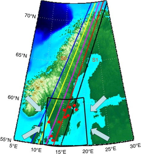
In view of the studies mentioned above and to facilitate similar studies in future, it is useful to characterise aerosol spatio-temporal and vertical distribution and to investigate its sensitivity to the large-scale meteorology. Here, we focus on the CALIOP sensor on board CALIPSO satellite that, for the first time, provides an opportunity to gather statistical information on the vertical structure of aerosols accurately. A noticeable feature of the orbital track of the CALIPSO satellite, that is of primary importance for us, is that its descending orbits follow the elongated major axis of Sweden as shown in Fig. 1 and passes the nearby major populated cities in Southern Sweden during the night-time. Spatial information from CALIPSO is limited, but at least one vertical cross-section over Sweden is available every 2–3 days along any one of the tracks shown in Fig. 1. Coupling this information with other sensors on board, the A-Train constellation of satellites would further enable the incorporation of spatial context and thermodynamics, thus helping to better understand aerosol spatio-temporal distribution. This aspect is exploited in the current study. In particular, an attempt is made to address the following points:

1. The seasonality in the vertical distribution of aerosols over Sweden

2. The role of temperature inversions in controlling their vertical distributions and

3. The impact of different wind directions on the vertical distribution of aerosols.

Fig. 1 Schematic of the CALIPSO orbits following the elongated major axis of Sweden. The red dots mark the most populated cities in southern Sweden.

2. Data sets

In the present study we use three data sets; aerosol information from CALIPSO, temperature profiles derived from the AIRS (Atmospheric InfraRed Sounder) instrument, and wind data from the ERA-Interim Reanalysis. A brief description of these data sets is given below.

CALIOP-CALIPSO data form the basis of the present study (Winker et al., 2009). We use 5 km aerosol layer product (Version 3) covering five years of data from June 2006 through May 2011 (Liu et al., 2009; Omar et al., 2009; Winker et al., 2009; Young and Vaughan, 2009). This data set is suitable for studying the large-scale statistical features in aerosol physical properties (e.g. Devasthale and Thomas, 2011; Devasthale et al., 2011). The data for both clear and cloudy sky conditions are used for the analysis. CALIOP cannot detect an aerosol layer below cloud if that cloud is optically thicker than 3. However, the sensor can detect the aerosol layer present over the cloud. In order to obtain realistic vertical distribution, we included both clear-sky aerosols as well as aerosols over clouds. It is worth pointing out that the observations showed that the frequency of aerosol-cloud overlap is very low over the study area (Devasthale and Thomas, 2011). A rigorous quality control is applied when using the data set. For example, an aerosol layer is analysed only if the feature is classified with high confidence and the value of Cloud-Aerosol-Discrimination (CAD) score is greater than 80 (Liu et al., 2009). This greatly reduces uncertainties related to aerosol-cloud misclassifications. It is to be noted that CALIOP may miss some of the optically thin aerosol layers over the study area. However, this underestimation is probably negligible compared to passive sensors. Relatively speaking, AODs are very low over Sweden compared to other polluted regions in the world. In this context, extra sensitivity of CALIOP to lower optical depths is very useful for our study area.

As shown in Fig. 1, the CALIPSO track roughly follows five well-defined pathways over Sweden during its descending passes. The vertical slices in the atmosphere from these corresponding tracks from east to west are designated as S1–S5. In this study, we examine the mean layer height of aerosols, AOD and the number of aerosol layers in the vertical for the period 2006–2011 along these five slices. We also evaluate how the vertical distribution of aerosols, layer AOD, the number of aerosol layers and the aerosol types in the region are affected by the winds. For the latter, we mainly focus on southern Sweden for the geographical region shown by the box and the wind direction as indicated by the arrows in Fig. 1.

The analysis is further complemented with observations from the AIRS sensor on-board AQUA satellite that provides information on thermodynamics. As both AIRS and CALIOP are a part of the A-Train constellation, the synergy between the two can be very useful in investigating the interplay of atmospheric thermodynamics and spatial and vertical distribution of aerosols and gases. Specifically for the present study, we use temperature retrievals from the daily level 3 data at 1° horizontal resolution. Although these retrievals are available at 24 vertical levels in the atmosphere (in the level 3 data version), we used retrievals reported at the eight lowermost levels (from the surface to 400 hPa) in the lower and middle troposphere, where temperature inversions are usually present. Further details of this data set, its applications in studying inversion characteristics can be obtained in Devasthale et al. (2010). We also use the estimates of zonal and meridional wind components from the ERA-Interim reanalysis project (Dee et al., 2011).

3. Results and discussion

In the present study, we investigate the following aspects of aerosol distribution over Sweden. First, we obtain the large-scale statistics of aerosol layer heights along the chosen five slices (Fig. 1) over Sweden during different seasons. We then focus on investigating the role of meteorology in influencing the observed distribution of aerosols. We specifically address temperature inversions, one of the dominant meteorological phenomena over Sweden, and wind direction and how these two affect the aerosol distribution.

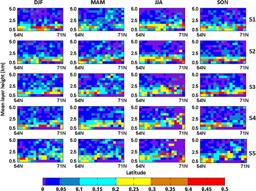
The frequency distribution of mean aerosol layer height with latitude is presented in Fig. 2 for different slices and seasons. Each 2D histogram shows the probability of observing aerosols at a particular height for each 1° latitude bin. Along the Y-axis the bin size (height interval) is 0.5 km. It is evident that approximately 50–70% of all aerosols are found below 1 km during the winter months in all the passes with respect to the surface and they are more evenly distributed in the layers above. North of 68N, the topography is characterised by mountainous terrain. Therefore, the boundary layer aerosols are found at higher altitudes compared to the southern latitudes. The surface elevation above mean sea level increases from S1 to S5 leading to increased aerosol altitudes from S1 to S5 northward of 68N. During the spring months, most of the aerosols lie below 1.5 km, but there are occasions when aerosols are homogeneously distributed in all the levels in S1 and S3 between 62N and 68N. However, during summer, the aerosols are lifted up to slightly higher levels (up to 2.5–3 km) because of convection induced by localised heating and stronger vertical mixing. This is more prominent in the latitude belt north of 63N. During SON months, the bulk of aerosols lie below 1.5 km. It is interesting to note that, among all seasons, the frequency of the occurrence of aerosols in the free troposphere (above 3 km) is highest during winter and spring compared to the rest of the year, especially towards northernmost latitudes. During half of the year, the boundary layer is decoupled from the free troposphere and the vertical mixing of polluted air masses is suppressed. The advected pollution in the free troposphere caused by the long-range (most likely isentropic) transport remains persistent in the free troposphere decoupled from the boundary layer. The circulation pattern also favours eventual transport of polluted Eurasian air masses to the Arctic via Scandinavian regions (Eckhardt et al., 2003; Stohl, 2006). Apart from the Eurasian sources, the intercontinental transport of aerosol precursor gases originating from North America (and subsequent aerosol formation and aging processes) and reaching over Scandinavia is also frequent and efficient during this half of the year (Stohl et al., 2002; Eckhardt et al., 2003; Stohl, 2006). For example, while inferring an indirect signal of long-range transport of carbon monoxide over Scandinavia during winter, Devasthale and Thomas (2012) recently showed that the pollution transport signal is most evident in the free troposphere (above 3 km) when the atmosphere is relatively unstable, winds are stronger and have a southerly component. Considering the tight connection of carbon monoxide with other anthropogenic aerosol precursor gases, it is expected that a similar signal (i.e. high frequency of aerosol layers in the free troposphere during winter) is also expected here. During summer, wet deposition and other scavenging processes are more efficient, thus explaining the observed lower frequency of aerosol layers in the free troposphere.

Fig. 2 Seasonal mean of the frequency distribution of the mean aerosol layer height with latitude.

For the investigations discussed hereafter, we focus on Southern Sweden (12E–20E, 55N–60N, the rectangular box in Fig. 1) since it accommodates majority of the Swedish population (top 10 populous cities). The probability of encountering layer AOD and total column AOD in the range 0.01–0.1 (in intervals of 0.01) averaged over Southern Sweden (the rectangular box in Fig. 1) and Northern Sweden (rest of the geographical area) for the four seasons is presented in Fig. 3a (top row) and Fig. 3c (bottom row), respectively, while the statistics on the number of aerosol layers found in the atmospheric profile is shown in Fig. 3b (middle row).

Fig. 3 Probability distribution of: (a) aerosol layer optical depths; (b) number of distinctive aerosol layers; and (c) total column aerosol optical depths for Southern and Northern Sweden.

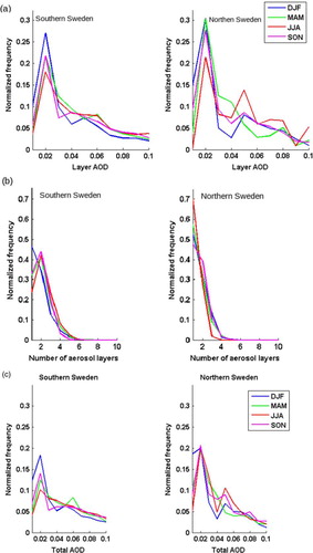
It is clearly seen that the majority of individual aerosol layers in the atmosphere have AODs less than 0.02 over both regions, with frequency of such events being highest in winter (narrow AOD pdf) and lowest in summer (broad pdf). However, over Southern Sweden, the probability of the occurrence of two aerosol layers in the atmospheric profiles is almost as high as the chances of observing one aerosol layer (Fig. 3b), while the presence of a single aerosol layer dominates over the Northern Sweden irrespective of the seasons. The layer AODs in the range 0.03–0.04 are most frequent during spring, while the AODs higher than those are commonly observed during summer over Sweden. The pdfs of the total column AOD shows similar features as the pdfs of layer AOD. This is expected mainly because of the presence of one, in most cases or, at the most two aerosol layers.

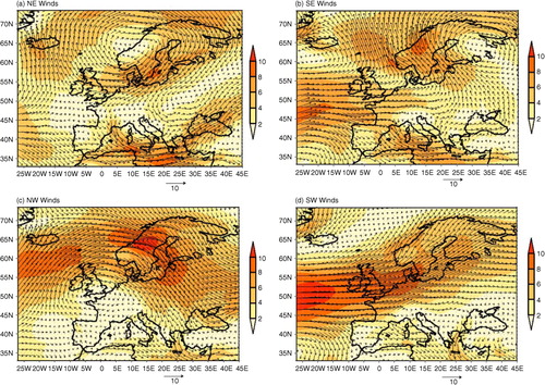
To investigate how meteorology affects the distribution of aerosols, first we analyse the daily 850 hPa winds from ERA-INTERIM Reanalysis (Dee et al., 2011) for the period 2006–2011 and classify them as north-easterly (NE), south-easterly (SE), north-westerly (NW) and south-westerly (SW). We select only those days for analysis when the winds prevail for at least three consecutive days in a particular direction. The composites of wind direction and strength for these four cases are presented in Fig. 4. It can be seen that the strongest winds occur when the winds are south-westerly with origins from North America and North Atlantic. The south-easterly winds transport air masses from central and eastern Europe over Sweden, whereas north-westerly winds have two distinct components, one approaching from the Arctic and the other from the Northeast Atlantic. A cyclonic flow is observed during the north-easterly winds over Sweden. The following paragraphs describe the variability in the vertical spacing between the aerosol layers observed, their distribution, layer AOD and the number of layers pertaining to the four wind directions mentioned above.

Fig. 4 The composites of wind strength and direction at 850 hPa for the four cases: (a) N-Easterly; (b) S-Easterly; (c) N-Westerly; and (d) S-Westerly.

The vertical distribution of aerosols during these four wind directions is shown in Fig. 5a. At a first glance, we notice that irrespective of the wind direction, the majority of aerosols lie below 2 km. When the winds have an easterly component, a secondary peak in the vertical distribution is observed. During north-easterly winds, a dual maxima of aerosols are located at 1 and 1.8 km, whereas during south-easterly winds, the maxima is seen at 0.5 and at 1 km. While during the NW, SW winds, the maxima of aerosols are located below the boundary layer. On a cautionary note, it should be pointed out that the number of aerosol profiles analysed is different for the different wind directions. Overall, the number of cases for a westerly wind component dominate (almost 60% for SW and almost 25% for NW component), while the least number of profiles are available when the winds are north-easterly (around 7%). This is not surprising considering the fact that the previous studies showed that the dominant wind direction over the study area is south-westerly and westerly (Chen, 2000; Linderson, 2001).

Fig. 5 (a) The vertical distribution of aerosols; (b) the vertical separation in the aerosol layers with respect to the wind directions; (c) cumulative distribution of the aerosols with height; (d) normalised frequency of the distribution of layer AOD; (e) the frequency of occurrence of the number of aerosol layers; and (f) normalised frequency of depolarisation ratio for the four selected wind directions (denoted by the different colours) for southern Sweden.

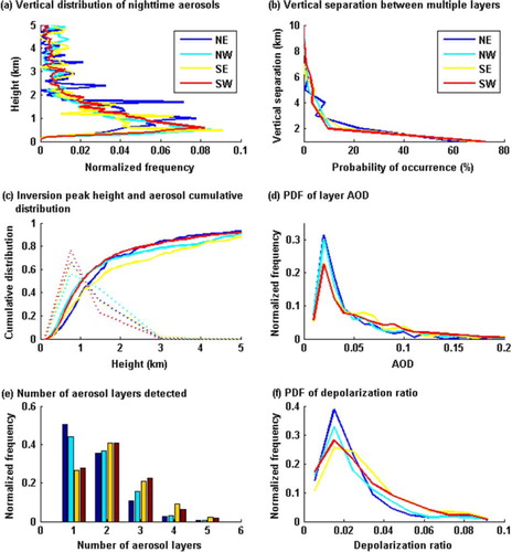
Apart from such composite vertical structure, it is useful to know how adjacent different aerosol layers are in the vertical. Figure 5b shows the vertical separation between aerosol layers when more than one aerosol layer is observed in the profile. It is expressed as the difference between the bottom height of upper aerosol layer and the top height of the lowermost layer. Interestingly the vertical separation follows the L-shaped distribution. In 60–70% of the cases, the aerosol layers are less than 1 km apart irrespective of the wind direction. There are, however occasions when the aerosol layers are widely spaced, but the likelihood of such events occurring is much less. It can be seen that, when the winds are north-easterly, there is a small likelihood that the vertical separation between aerosol layers is around 3–5 km. This could be due to the fact that when the winds are north-easterly, they are cyclonic in nature (Fig. 4), thereby transporting aerosols from distant sources into southern Sweden for those specific cases.

Figure 5c presents the cumulative distribution of the aerosols with respect to height for the box mentioned above and for the four selected wind cases. The dashed lines represent the height of the inversion peak during these four wind directions. Irrespective of the wind direction, about 30–50% of the aerosols lie below the inversion layer peak at 1.2 km with a slightly large fraction of the aerosols when the winds have a westerly component. Figure 5d shows the normalised frequency distribution of layer AOD during these different wind directions represented by the different coloured lines. The layer AOD peaks around 0.025 irrespective of the wind direction, but, the frequency of occurrence of such cases is more when the winds are NE and NW (around 30%) compared to when the winds have the southerly component (around 20%). Also, the layer AOD is less than 0.08 for more than 80% of the time. When the winds have a southerly component, aerosol layers with AOD greater than 0.05 are more frequent. There are cases when the layer AOD exceeds 0.15, but the probability of such cases is very low. We further analysed the frequency of occurrence of the number of aerosol layers for the selected wind directions as shown in Fig. 5e. When the winds have a northerly component, a single aerosol layer is predominantly observed, while during southerly winds, two layers are more common. Three or more layers are often observed when winds have a southerly component. The lidar depolarisation ratio can be used to understand the physical nature and morphology of aerosols (Omar et al., 2009). For example, non-spherical aerosols (dust) and polluted aerosols after undergoing transport, coating and aging processes can have a higher depolarisation ratio than the clean spherical aerosols. Figure 5f shows the normalised frequency of depolarisation ratio for aerosol layers under different wind conditions. There is a clear tendency that when the winds have a southerly component, aerosol layers have a high depolarisation ratio. A similar tendency is also observed in the distribution of layer integrated attenuated backscatter at 532 nm (not shown).

Finally, it is worth pointing out that, if we do a synthesis of all results mentioned above with previous published studies based on in-situ and chemical transport model data that underline the importance of long-range transport from continental Europe (Stohl et al., 2002; Eckhardt et al., 2003; Stohl, 2006; Devasthale and Thomas, 2012; and references therein), they fit together quite well. For example, when the southerly winds (SE and SW) prevail, two or more aerosol layers and higher frequency of high AOD values are observed. The depolarisation ratio and attenuated backscatter of these layers are also higher. This is consistent with the fact that the winds over Sweden are predominantly of southerly origin and have a transport history from continental Europe, northern North Atlantic, and/or North America, which is partly visible in Fig. 4. Previous studies (Stohl et al., 2002; Eckhardt et al., 2003; Stohl, 2006) showed that the major pathway of an eventual long-range transport of pollutants from these regions to the Arctic passes over Scandinavia during winter as well as summer half of the year. Especially strong episodic intrusions via this pathway would lead to higher frequency of the right hand tail of the AOD pdfs for the SW and SE cases shown in Fig. 5d. On the other hand, the relatively cleaner air from the NE and NW directions leads to higher frequency of low AOD values (also evident in Fig. 5d). The NE winds seem to show cyclonic behaviour, centred on the western coast of Norway, drawing polluted air masses from the northern and eastern parts of Europe at lower altitudes and from the North Atlantic at higher altitudes. This could partly explain the secondary peak at relatively higher altitude in the vertical distribution of aerosol layers in the NE case (Fig. 5a).

4. Conclusions

Aerosols play a crucial role in the Earth system. They have multiple effects on our climate through their direct and indirect interactions with radiation. Furthermore, they influence air quality and hence, public health. One of the key knowledge gaps when quantifying aerosol impact on climate and air quality is our limited understanding of their vertical distribution. This is especially true in the case of high latitude countries such as Sweden where passive imagers on board satellites have inherent difficulties in retrieving reliable aerosol information, and where ground-based measurements are inadequate.

The active aerosol lidar on board CALIPSO is helping in closing this knowledge gap by providing reliable vertical distribution of aerosols globally. The descending (night-time) orbital tracks of the CALIPSO satellite are aligned along the elongated semi-major axis of Sweden. This favourable combination of geographical alignment and orbital track allows observation of vertical structure of aerosols along meridional direction at least once every 2–3 d over Sweden. In addition, combining aerosol information with other spatially and temporally collocated retrievals of temperature from the A-Train constellation (together with wind data) is extremely useful in understanding how the large-scale meteorology influences aerosol vertical distribution. These aspects are studied here using five years of CALIPSO data (2006–2011).

It is found that the majority of aerosols (up to 70%) are located within 1 km above the surface in the lowermost troposphere, irrespective of the season. Convection and stronger mixing lift aerosols to slightly higher levels in summer. However, in the upper free troposphere above 3 km, aerosol layers are frequently observed in the winter half of the year compared to the summer half.

The investigations of aerosol characteristics under different wind conditions over Sweden reveal the following aspects. Multiple aerosol layers are most frequent over southern Sweden and have higher AOD values when the winds are southerly. The depolarisation ratio and integrated attenuated backscatter values for aerosol layers are also higher when the winds have a southerly component. About 30–50% of all aerosol layers are located below the level where temperature inversions peak. It is also found that, when multiple aerosol layers are present in the atmosphere, the vertical separation between them is less than 1 km in the majority of cases (60–70%). These results underscore the important role of transport from continental Europe and the North Atlantic over Scandinavia. Future work will involve investigating statistical co-variations of other short-lived climate pollutants with aerosols and looking at how these statistics would be simulated by a chemistry transport model.

5. Acknowledgements

This work has been funded through the CLEO project (Climate Change and Environmental Objectives) from the Swedish Environmental Protection Agency and through MACCI project (Modelling Aerosol-Cloud-Climate Interactions and Impacts) from the Swedish Research Council. M. Kahnert acknowledges funding from the Swedish Research Council (project 621-2011-3346). Authors gratefully acknowledge the efforts of CALIPSO and AIRS science teams for providing their data sets available for research. These data were obtained from the ASDC/NASA Langley and NASA GES DISC facilities. ERA-Interim data were obtained from the ECMWF data centre. We also thank Matthias Tesche (ITM, Stockholm University) for valuable feedback. The Swedish National Space Board supported this work.

References

- Chen D . A monthly circulation climatology for Sweden and its application to a winter temperature case study. Int. J. Clim. 2000; 20: 1067–1076.
- Dee D. P , Uppala S. M , Simmons A. J , Berrisford P , Poli P , co-authors . The ERA-Interim reanalysis: configuration and performance of the data assimilation system. Q. J. Roy. Meteorol. Soc. 2011; 137: 553–597.
- Devasthale A , Thomas M. A . A global survey of aerosol-liquid water cloud overlap based on four years of CALIPSO-CALIOP data. Atmos. Chem. Phys. 2011; 11: 1143–1154.
- Devasthale A , Thomas M. A . An investigation of statistical link between inversion strength and carbon monoxide over Scandinavia in winter using AIRs data. Atmos. Environ. 2012; 56: 109–114.
- Devasthale A , Tjernström M , Omar A. H . The vertical distribution of thin features over the Arctic analysed from CALIPSO observations. Part II: aerosols. Tellus. B. 2011; 63: 86–95.
- Devasthale A , Willen U , Karlsson K.-G , Jones C. G . Quantifying the clear-sky temperature inversion frequency and strength over the Arctic Ocean during summer and winter seasons from AIRS profiles. Atmos. Chem. Phys. 2010; 10: 5565–5572.
- Eckhardt S , Stohl A , Beirle S , Spichtinger N , James P , co-authors . The North Atlantic Oscillation controls air pollution transport to the Arctic. Atmos. Chem. Phys. Discuss. 2003; 3: 3223–3240.
- Genberg J , Hyder M , Stenström K , Bergström R , Simpson D , co-authors . Source apportionment of carbonaceous aerosol in southern Sweden. Atmos. Chem. Phys. 2011; 11: 11387–11400.
- Guibert S , Matthias V , Schulz M , Boesenberg J , Eixmann R , co-authors . The vertical distribution of aerosol over Europe – synthesis of one year of EARLINET aerosol lidar measurements and aerosol transport modeling with LMDzT-INCA. Atmos. Environ. 2005; 39: 2933–2943.
- Gustafsson M , Franzén L . Inland transport of marine aerosols in southern Sweden. Atmos. Environ. 2000; 34: 313–325.
- Hoff R. M , Christopher S. A . Remote sensing of particulate pollution from space: have we reached the promised land?. J. Air. Waste. Manag. Assoc. 2009; 59: 645–675.
- Linderson M.-L . Objective classification of atmospheric circulation over southern Scandinavia. Int. J. Clim. 2001; 21: 155–169.
- Liu Z , Vaughan M. A , Winker D. M , Kittaka C , Kuehn R. E , co-authors . The CALIPSO lidar cloud and aerosol discrimination: version 2 algorithm and initial assessment of performance. J. Atmos. Ocean. Tech. 2009; 26: 1198–1213.
- Omar A. H , Winker D. M , Vaughan M. A , Hu Y , Trepte C. R , co-authors . The CALIPSO automated aerosol classification and lidar ratio selection algorithm. J. Atmos. Ocean. Tech. 2009; 26: 1994–2012.
- Paciorek C. J , Liu Y . Assessment and statistical modeling of the relationship between remotely sensed aerosol optical depth and PM2.5 in the eastern United States. Res. Rep. Health. Eff. Inst. 2012; 167: 5–83.
- Rodhe H , Persson C , Akesson O . An investigation into regional transport of soot and sulfate aerosols. Atmos. Environ. 1972; 6: 675–693.
- Sporre M. K , Glantz P , Tunved P , Swietlicki E , Kulmala M , co-authors . A study of the indirect aerosol effect on subarctic marine liquid low-level clouds using MODIS cloud data and ground-based aerosol measurements. Atmos. Res. 2012; 116: 56–66.
- Stohl A . Characteristics of atmospheric transport into the Arctic troposphere. J. Geophys. Res. 2006; 111: D11306.
- Stohl A , Eckhardt S , Forster C , James P , Spichtinger N . On the pathways and timescales of intercontinental air pollution transport. J. Geophys. Res. 2002; 107(D23): 4684.
- Tunved P , Nilsson E. D , Hansson H.-C , Ström J , Kulmala M , co-authors . Aerosol characteristics of air masses in Northern Europe: influences of location, transport, sinks and sources. J. Geoph. Res. 2005; 110: D07201.
- Tunved P , Hansson H.-C , Kulmala M , Aalto P , Viisanen Y , co-authors . One year boundary layer aerosol size distribution data from five Nordic background stations. Atmos. Chem. Phys. 2003; 3: 2183–2205.
- van Donkelaar A , Martin R. V , Brauer M , Kahn R , Levy R , co-authors . global estimates of ambient fine particulate matter concentrations from satellite-based aerosol optical depth: development and application. Environ. Health. Perspect. 2010; 118: 847–855.
- Winker D. M , Vaughan M. A , Omar A , Hu Y , Powell J. A . Overview of the CALIPSO mission and CALIOP data processing algorithms. J. Atmos. Ocean. Tech. 2009; 26: 2310–2323.
- Young S. A , Vaughan M. A . The retrieval of profiles of particulate extinction from Cloud Aerosol Lidar Infrared Pathfinder Satellite Observations (CALIPSO) data: algorithm description. J. Atmos. Ocean. Tech. 2009; 26: 1105–1119.