The long-term variability of atmospheric ozone from the 50-yr observations carried out at Belsk (51.84°N, 20.78°E), Poland

Abstract

Total ozone (TO₃) and ozone vertical profile (by the Umkehr method) have been measured at Belsk (51.84°N, 20.78°E), Poland, since March 1963. The monthly mean data are analysed for the long-term changes in the period 1975–1996 and 1997–2012, that is, in the increasing and decreasing phases of the ozone-depleting substances (ODS) concentration in the mid-altitude stratosphere over the NH mid-latitudes. Standard explanatory variables are selected for the ozone variability attribution to chemical and dynamical processes. A triad of regression models with various formulae for the trend term is examined to get a synergetic effect. The trend term could be: (1) proportional to ODS, (2) piecewise linear (with the turning points in 1975 – the trend onset and in 1997 – the trend overturning), (3) represented by any smooth curve fitted to the ozone time series having ‘natural variations’ removed. Confirming the results from previous studies on the midlatitudinal ozone, the analyses show a weakening of the TO₃ trend and the statistically significant positive trend in the upper stratospheric region (33–43 km) since 1997. The TO₃ depletion in summer and autumn for the period 1997–2012 is found in the Umkehr data due to the ozone decrease in the lower and mid-stratosphere. A novel statistical-simulation-based test is proposed. It uses the bootstrap sample of the smooth trend pattern to calculate statistical significance of hypotheses for the trend variability. The test corroborates the results of the regression models and shows strengthening of the ozone negative trend in summer and autumn, disclosed in the Umkehr data, since about 2005.

• Ozone
• trend
• ozone recovery
• column amount
• vertical profile
• statistical model

1. Introduction

The ozone issue has been an important research topic since the early 1970s findings of a threat to the ozone layer by man-made substances (Johnston, 1971; Crutzen, 1973; Molina and Rowland, 1974). The discovery of the ozone hole over the Antarctica (Chubachi, 1984; Farman et al., 1985) and significant downward trend over the northern mid-latitudes revealed by the Ozone Trend Panel (WMO, 1989) alarmed scientists and the public of possible increase of the surface ultraviolet (UV) radiation, which has a harmful impact on humans and ecosystems. It has triggered unprecedented international cooperation between politics, scientists and industrialists to save the ozone layer. Finally, due to joint efforts of the United Nations countries, the Montreal Protocol (MP) on the protection of the ozone layer was agreed on 16 September 1987 and came into effect on 1 January 1989.

Ozone-depleting substances (ODS) contain bromine, chlorine, fluorine, carbon and hydrogen in varying proportions. The combined ozone-destructive potential of these chemicals is expressed by the equivalent effective stratospheric chlorine (EESC) concentration (e.g. Newman et al., 2007). The EESC changes with time are used to monitor anthropogenic forcing on the ozone layer and to find out the effectiveness of the MP regulations on ODS production limits.

MP underwent several amendments in subsequent years and appeared to be very effective in reducing the ODS level. Now, more than 20 yr later, the effectiveness of the MP for the protection of the layer is still a discussed issue. The statistical analyses of the observed (satellite- and ground-based) ozone data and the ozone modelling by global chemical transport models have been used to find the anthropogenic component of the ozone trend (WMO, 2011).

Recent WMO reports on the state of ozone layer (WMO, 2007, 2011) pointed out that the increase of ODS level was mostly responsible for the ozone depletion in the extratropics in the 1980s and early 1990s. The ODS level in the stratosphere has begun to decline since the mid-1990s. This triggered searching for the corresponding changes in the long-term ozone pattern. WMO (2007) has defined the following stages of the ozone recovery: (1) a slowing in the downward trend; (2) onset of the statistically significant positive trend in the ozone data having ‘natural’ variations removed and (3) reaching the pre-1980 ozone levels in the stratosphere.

Multi-decadal homogeneous ground-based observations of total ozone (TO₃) and the ozone vertical profile by the ozone soundings or the Umkehr measurements are basic sources to delineate ozone variability with different time scales ranging from the intra-day oscillations up to decadal trends. There are only a few stations in Europe with the continuous ozone observations for an approximately 50-yr period or longer. These are Arosa, Belsk, Hradec Kralove, Lerwick, Lisbon, Potsdam and Reykjavik. TO₃ and the ozone vertical profiles by the Umkehr measurements have been carried out continuously up to now only at Arosa and Belsk. This article focuses on the analysis of the Belsk's ozone data to estimate trends in two consecutive periods, that is, in the period of the ODS increase (1975–1996) and decrease (1997–2012), for the detection to what extent the stratospheric ozone recovers over the site.

2. Ozone data

Observations of the atmospheric ozone, column ozone and the ozone vertical profile by the Umkehr method have been carried out at Central Geophysical Observatory Institute of Geophysics Polish Academy of Sciences, Belsk (51.84°N, 20.78°E), since 23 March 1963 until now by the same instrument Dobson spectrophotometer No. 84.

The quality of the Belsk's ozone time series has been tested during frequent international intercomparison campaigns (e.g. Belsk 1974, Potsdam 1979, Arosa 1986 and 1990) with the world standard instrument No. 83 (e.g. WMO, 1996). Subsequent campaigns (2001, 2005, 2009) took place at the regional Dobson calibration centre established in 2000 at the Meteorological Observatory Hohenpeissenberg, Germany. The centre provides the European sub-standard (the Dobson instrument No. 64) and closely cooperates with World Dobson Ozone Calibration Center at NOAA, Boulder, USA, and the Solar and Ozone Observatory at Hradec Kralove, Czech Republic. The new calibration constants, the so-called R-N tables, were retrieved and applied to the previous and current ozone observations if a large bias was found relative to the standard instrument measurements. The instrument quality control was also assured by comparisons with the collocated Brewer spectrophotometer measurements (since 1992) and with the satellite data taken during the Belsk's station overpasses (Rajewska-Więch et al., 2006). The Belsk's TO and the Umkehr ozone profiles were used in various trend analyses starting from the paper of Degórska et al. (1989) showing negative trend in the Belsk's TO₃ in winter.

2.1. Total ozone

The TO₃ values are calculated using both the fundamental direct sun and the less precise zenith blue or zenith cloud measurements of spectral irradiance for the wavelength pair, one with strong and another with weak absorption of the solar UV radiation (Dobson, 1957). The measurements are performed a few times per hour during the day with special focus on the direct sun observations near local noon because of their highest accuracy. The data quality procedures of the Dobson measurements were introduced in the mid-1970s and the data quality of earlier measurements, 1963–1974, that is, up to the year of the first international intercomparison at Belsk, it might be lower (Dziewulska-Łosiowa et al., 1983; Degórska and Rajewska-Więch, 1991; Degórska et al., 1995).

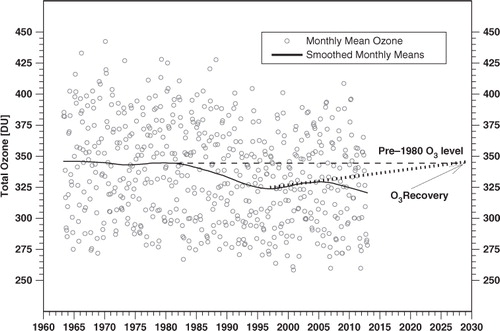
Figure 1 shows TO₃ monthly means calculated from the daily mean values obtained in the period 23 March 1963–31 December 2012. The smoothed series by locally weighted scatterplot smoothing (LOWES, Cleveland, 1979) reveals the following stages of the long-term variability of the Belsk's TO₃: a constant level period up to the early 1980s, the next decline stopped around mid-1990s, since then an oscillation with the maximum around 2005 and the minimum, which is comparable to that in 1996, in the end of the time series. The recent behaviour of the Belsk's ozone is quite surprising as the second stage of the ozone recovery is rather expected from the recent ODS decrease than the oscillation around the mid-1990s level. The rate of ozone increase since the mid-1990s up to the early 2000s suggested that the ozone recovery would occur around 2030 at Belsk. However, a slight TO₃ decline since 2005 up to the end of the ozone series disallows to make such a simple estimation of the recovery time.

Fig. 1 Total ozone monthly means from the Dobson spectrophotometer measurements at Belsk in the period March 1963−December 2012. The solid line shows the long-term variability in the data by the LOWES smoother. Two dashed lines, horizontal line showing the pre-1980 ozone level and the sloped line, are shown for an estimation of the recovery time based on the ozone increase rate in the period 1997–2005.

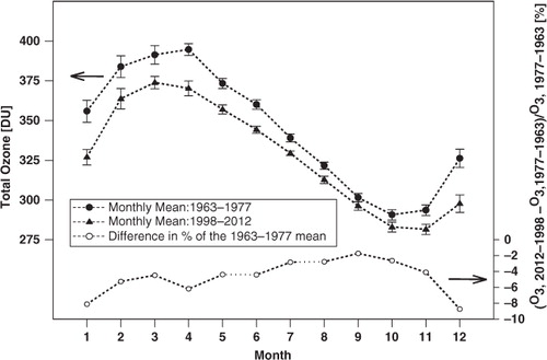
Comparison between the long-term TO₃ monthly means calculated from the monthly TO₃ values taken at the first (1963–1977) and last (1998–2012) 15-yr period of the Belsk's measurements (Fig. 2) shows that the ozone loss at Belsk is seasonally dependent with the maximum depletion in December and January of ~8% and the minimum depletion in September of ~2% relative to the TO₃ level in the first period.

Fig. 2 The long-term total ozone monthly means for the first (1963–1977) and last (1998–2012) 15-yr period of the ozone observations at Belsk and the relative monthly differences between these means as a percent of the means in the former period.

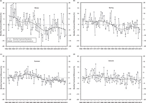
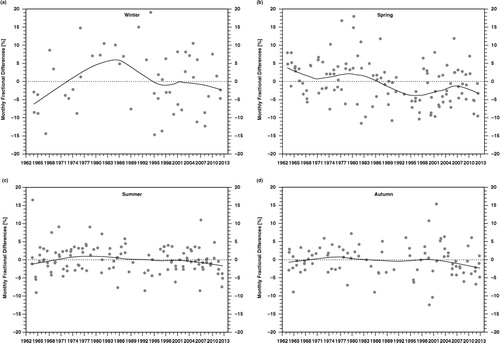
Figure 3 illustrates the TO₃ variability within each season of the year. The deviations of TO₃ from its the long-term 1963–2012 monthly means for the four seasons of the year show a common feature, that is, a decline from the end of 1970s to the mid-1990s, and a kind of stabilisation afterwards. This stabilisation means an appearance of a long-term oscillation with the maximum around 2005 in the winter/spring TO₃ or a continuation of a slight ozone depletion in summer and autumn.

Fig. 3 The monthly differences of total ozone relative to the long-term (1963–2012) means as a percent of the long-term means: (a) winter – DJF; (b) spring – MAM; (c) summer – JJA and (d) autumn – SON.

2.2. Vertical ozone profile

Monitoring of the ozone vertical profiles by the Umkehr observations is possible for cloudless weather conditions for a few hours after sunrise or before sunset. The ratio of measured zenith-sky radiance at a UV wavelength pair, one strongly and other weakly absorbing, is obtained from the Umkehr observations by the ground-based spectrophotometers. The wavelength pair radiances are measured from zenith sky under cloudless conditions for a set of discrete solar zenith angles (SZAs) changing from 60 to 90° (for previous Umkehr retrieval algorithm proposed, see Mateer and DeLuisi, 1992) or starting from any SZA in the range 60–80° and ending at 90° (for recently proposed UMK04 retrieval algorithm, see Petropavlovskikh et al., 2005). In this article, the Umkehr profiles are based on UMK04 retrieval algorithm using C-wavelength pair (311.5 and 332.4 nm) with the lowest SZA of 70°.

The Umkehr retrieval partitions column ozone into 10 Umkehr layers that are divided into equal log-pressure vertical intervals, starting at the surface (~1013 hPa) and extending to layer 10 (from ~1 hPa level up to the top of the atmosphere). The ozone content above ~10 km is reported in ~5 km thick layers. Although the Umkehr retrieval provides the ozone content in 10 layers, because of broad and strongly overlapping weighting functions, as well as finite measurement errors, the retrieval contains only a few independent pieces of information. Thus, in the article we analyse the ozone content in the consecutive Umkehr layers: 2+3+4 (10.3–23.5 km, lower stratosphere), 5+6 (23.5–32.8 km, middle stratosphere) and 7+8 (32.8–42.6 km, upper-stratosphere).

Measurement errors, smoothing errors, forward-model errors and inverse model errors for the Umkehr retrieval were discussed in the SPARC (1998) report. Fioletov et al. (2006) showed that the measurement uncertainties for the Umkehr observations depend on altitude, that is, ~8% for 0–20 km integrated ozone and ~5% for 20–32 km. Petropavlovskikh et al. (2008) analysed multiple comparisons between the Umkehr profiles by the Dobson instruments and they found the bias in the measured Umkehr profiles by various Dobson instruments and multiple retrievals that could not be easily explained. Thus, it seems that the trend analyses of the Umkehr data should be treated with care.

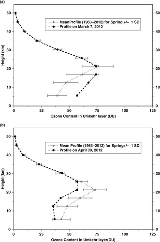
The Umkehr algorithm is able to retrieve the ozone profile starting from a priori profiles. Figure 4 shows examples of the Umkehr ozone profiles for 2 d with a large positive and negative departure from the long-term (1963–2012) mean profile in the lowermost Umkehr layers up to the mid-stratosphere. The Umkehr profiles are taken at Belsk only during clear-sky conditions. The mean number of Umkehr observations per month is the lowest in December (1 d) and the highest in May (6 d). Thus, it seems possible that the monthly mean Umkehr profile averaging only a few daily profiles is not representative for the whole month.

Fig. 4 Examples of the Umkehr ozone profiles superposed on the long-term (1963–2012) monthly mean profiles: (a) with a positive decline in the lower stratosphere – 7 March 2012 and (b) with a negative decline in the lower stratosphere – 30 April 2012.

Figure 5 presents the long-term TO₃ variability in the four seasons of the year based on the TO₃ data taken during days when weather permitted the Umkehr observations. Comparison of Fig. 3a and Fig. 5a shows that the long-term TO₃ pattern for winter, which is calculated using only the Umkehr days, does not match with that derived from all-sky standard TO₃ measurements by the Dobson spectrophotometer. Therefore, the winter and the year-round Umkehr trends are not presented in this article.

Fig. 5 The same as Fig. 3 but for the subset of the total ozone values taken only in days with the Umkehr observations.

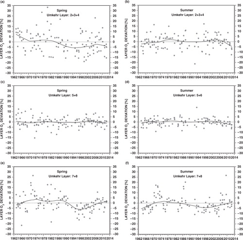
The long-term variability of the ozone content in selected layers of the atmosphere is shown in Fig. 6 for the lower-, mid- and upper-stratosphere in spring and summer. The ozone depletion at Belsk before 1997 appears in the lower (only in spring) and the upper stratosphere. Since then, the apparent upward ozone tendency is found only in the upper stratosphere. The mid-stratosphere ozone appears to be relatively constant for the whole period of the Belsk's observations.

Fig. 6 The monthly differences of ozone content in the combined Umkehr layers in the period 1963–2012 relative to the long-term means for that period as a percent of the long-term means: spring (left-hand side), summer (right-hand side).

3. Trend analyses

3.1. Trend model definition

Considering our previous studies (Krzyścin and Rajewska-Więch, 2009; Krzyścin, 2012), a triad of the trend models is used to find the long-term ozone change in the periods 1975–1996 (increasing the ODS level) and 1997–2012 (decreasing the ODS level forced by regulations of the MP and its subsequent amendments). It is assumed that fluctuations in the atmospheric ozone are due to long-term changes in the atmospheric chemistry (mostly related to changes in ODS) and due to various dynamical processes affecting the ozone transport. Thus, the ozone variability is modelled as the sum of chemical and dynamical components described as follows:1

where: ΔO₃(t) is the ozone fractional deviation in running month t,2

t=(year–1963)×12+M, year={1963, …, 2012}, O₃(t) is TO₃ (or ozone content in the Umkehr layer) monthly mean in month t, O₃(M) is the long-term (1963–2012) monthly mean for calendar month M corresponding to running month t, Trend(t) represents a slowly varying component (trend) of the ozone time series, Dynamics(t) is a linear combination of the proxies, X _i (t), chosen by the standard stepwise regression procedure, which allows to select a subset of the proxies that significantly affects model (1) outcome,3

where constants ϕ _i are calculated by a multi-linear statistical analysis. Standard stepwise regression is used to eliminate redundant variables from a set of potential proxies. Noise(t) represents the noise term that can be partially linked to a short-term dynamical forcing causing some autocorrelations in the noise term (usually with the 1-month lag).

3.2. Ozone regressors

The common approach in analyses of the ozone variability is searching for variables that could be used for an attribution of the long-term and/or short-term ozone variability. Following recent studies (e.g. Krzyścin et al., 2005; Mäder et al., 2007; Vyushin et al., 2007; Wohltmann et al., 2007; Harris et al., 2008; Yang et al., 2009; Rieder et al., 2011; Nair, 2012; Rieder et al., 2013), we examine the number of proxies parameterising chemical and dynamical processes potentially responsible for the ozone variability over a midlatitudinal NH station. These are: (1) EESC for the attribution of the stratospheric ODS influence on ozone, (2) the zonal component of wind at 30 and 50 hPa averaged over the tropics for the Quasi Biennial Oscillation (QBO) attribution, (3) the Arctic Oscillation (AO) Index, (4) Penticton/Ottawa 2800 MHz solar flux to search for the 11-yr solar cycle effects, (5) the El Nino/Southern Oscillation (ENSO) index, which is based on sea-surface temperature (SST) anomaly in the Niño-3.4 region, used to account for the global atmosphere disturbances induced by quasi-periodical SST fluctuations in the equatorial Pacific, (6) stratospheric aerosol optical depth at 550 nm to describe the amount of stratospheric aerosols leading to the ozone depletion through a series of catalytic chemical reactions after strong volcanic eruption, (7) detrended meteorological variables over the Belsk's station comprising a temperature of 50 and 10 hPa level, and the tropopause pressure to account for the month-to-month ozone variations due to local dynamical processes. Table 1 shows the web addresses for the proxies used.

Table 1. The explanatory variables used in the study

Data	Source
QBO at 30 hPa and 50 hPa	NOAA National Weather Service Climate Prediction Center http://www.cpc.noaa.gov/data/indices/qbo.u30.index
AO Index	http://www.cpc.ncep.noaa.gov/products/precip/CWlink/daily_ao∣_index/ao_index.html
ENSO index	http://www.cpc.ncep.noaa.gov/products/analysis_monitoring/en∣sostuff/detrend.nino34.ascii.txt
EESC based on WMO Scenario A1_2010 mid-latitudes: mean age of air 3 yr., age of air-spectrum width 1.5 yr	NASA Goddard Institute for Space Studies http://acdb-∣ext.gsfc.nasa.gov/Data_services/automailer/
Penticton 2800 Hz Solar Flux	NOAA National Geophysical Data Center ftp://ftp.ngdc.noaa.gov/STP/SOLAR_DATA/SOLAR_RADIO/∣FLUX/Penticton_Adjusted/monthly/MONTHLY.ADJ
Stratospheric aerosol optical depth at 550 nm – zonal mean for ~50°N latitude	http://data.giss.nasa.gov/modelforce/strataer/
Temperature at 50 hPa and 10 hPa levels, and the tropopause pressure interpolated from the gridded data	CDAS-NCEP/NCAR Reanalyses 4x daily 1948–2012 ∣ Annual Meteorological Statistics: http://nomad3.ncep.noaa.gov/cgi-bin/pdisp_6p_r1.sh

3.3. Triad of the regression models

Model (1) is run separately for the winter (DJF), spring (MAM), summer (JJA) and autumn (SON) subset of the year data, and for the year-round (J … D) data. The following formulae are selected for a description of the trend term:

• EESC model

4

where EESC(t) is time series of the ODSs concentration in the stratosphere, t ₁ =1975 denotes onset of the ozone trend, the regression constant, α, depends on season of the year,

• Piecewise linear trend (PWLT) model

5

Trend(t) is a broken line beginning in 1963 with zero slope up to 1975 (i.e. up to the assumed onset of the anthropogenic trend and beginning of the Belsk's Dobson calibration procedure with the standard Dobson spectrophotometer) and afterwards the trend shape is described by two lines with the turning point in 1997 (i.e. the supposed year of the ozone recovery onset in the midlatitudinal stratosphere), ɛ _1975°(t)=1 if t≥1975 and 0 otherwise, ɛ _1997°(t)=1 if t≥1997 and 0 otherwise. Regression coefficients, β, and γ, are seasonally dependent, β and β+γ represent the rate of ozone change (% per decade) in the periods 1975–1996 and 1997–2012, respectively.

• Flexible (FLEX) model

6

where Smooth(t) is a trend curve, that is smooth function that is filtered out from the residual time series of model (1), Resid(t), which remains after subtracting dynamically driven variations by EESC or PWLT model from the original series ▵O₃(t),7

This model is called flexible trend model as the trend curve is not a priori defined but it is extracted from the time series of residuals. The level of smoothing of Resid(t) time series by LOWES smoother (Cleveland, 1979) to extract the smooth component, Smooth(t), is chosen to filter out the short-term oscillations with periodicities up to about decade.

The EESC model is well suited for searching anthropogenic components of the long-term oscillations related to the ODS changes in the stratosphere. Since 1987, ODS variability has been controlled by regulations of the MP (and its further amendments) to protect the ozone layer. It seems that the EESC model could be used to find the effectiveness of this international treaty. However, EESC trend describes the stratospheric chlorine and bromine effects on ozone layer due to gas-phase chemistry. Heterogeneous chemistry on polar stratospheric clouds also has an impact on the midlatitudinal ozone due to the Arctic air mass intrusion to this region after the polar low break (Fioletov and Shepard, 2005).

Moreover, the EESC pattern is not unique as it could be defined in dependence on air-age and air-spectrum width (see Table 1). The relationship between ozone and EESC is based on the data collected in the period of large changes in these variables (late 1980s and early 1990s). The trend component due to ODS changes is difficult to extract by other trend models in a period of small EESC change (e.g. 1997–2012). Trends by PWLT and FLEX model may be a superposition of chemical and dynamical components due to unknown yet forcing on the ozone layer. Thus, the trends estimated by these models cannot be linked only to the effect of man-made chemicals being included in the EESC calculations.

The basic advantage of FLEX model is an extraction of the long-term pattern from the data having the ‘natural’ variations removed. The trend estimation by FLEX model is not constrained by any initial assumption of the trend curve shape. The replica of the ODS time series (with opposite sign) and the PWLT are chosen for EESC and PWLT models, respectively. Therefore, FLEX has the largest freedom in description of the trend shape but it needs a priori defined smoothness level. Moreover, calculation of the trend uncertainty is time consuming and requires an application of a resampling technique.

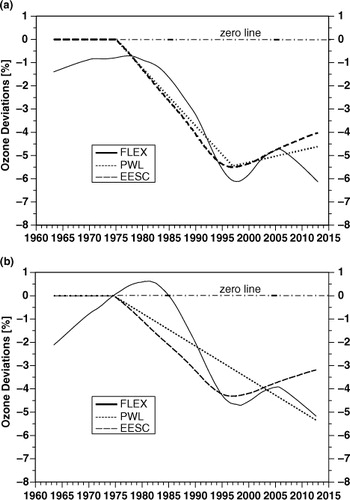
The trend models examined here have been extensively used in previous estimates of the long-term ozone changes: EESC model (e.g. WMO, 2007; Harris et al., 2008), PWLT (e.g. Reinsel et al., 2005; Yang et al., 2009) and FLEX (e.g. Harris et al., 2001; Krzyścin and Rajewska-Więch, 2009). Figure 7 shows examples of the trend pattern by all the models for the winter and the summer subset of the monthly data. The trend pattern by EESC follows the shape of ODS time series of opposite sign. The value of regression coefficient, α , is a result of the TO₃–ODS anti-correlation in the period of substantial ODS increase and ozone decrease (1975–1996). Thus, it leads to the ozone recovery in the declining phase of ODS level in the stratosphere. PWLT and FLEX model do not support the ozone increase in summer during the declining ODS phase. For example, PWLT model shows continuously declining TO₃ tendency since 1975. FLEX trend shows a more complicated picture of the long-term ozone pattern with a local maximum around 2005.

Fig. 7 The trend curves used in the examined models of the ozone variability (dashed – EESC, dotted – PWLT, solid – FLEX): (a) winter (DJF) total ozone, (b) summer (JJA) total ozone.

The trend values in % per decade are analysed for the periods 1975–1996 and 1997–2012. These values are directly provided by the PWLT model as the regression coefficient β and β+γ, respectively. Whereas for EESC and FLEX models, the linear trend equivalent is calculated. First, the differences between the trend curve values in 1975, 1996 and 2012 are obtained. The trend curves are defined as α×(EESC(t)-EESC(t ₁)) and Smooth(t) for EESC and FLEX model, respectively. Next, the differences are divided by the time span to have linear trend equivalent values for the periods 1975–1996 and 1997–2012.

The trend errors by EESC and PWLT model are calculated in a standard way taking into account the 1-month autocorrelation in Noise(t) term (Weatherhead et al., 1998; Storch and Zwiers, 1999), Errors for the trend values by FLEX model are from the block bootstrap technique using N=10000 samples of hypothetical Smooth* _n (t) time series derived by the LOWES smoothing of bootstrapped Resid(t) time series, Resid* _n (t),8

where Noise* _n (t) is the n-th hypothetical representative of Noise*(t) term [see eq. (7)] that is composed from consecutive 3-month seasonal blocks randomly drawn from Noise*(t) term. The methodology for calculating trend error based on bootstrap samples is described in more detail in our previous paper (Krzyścin, 2006).

3.4. Test of trend sign

Usually the long-term ozone changes are discussed based on trend values and their errors for selected periods. Here, we also examine another possibility focusing on the trend sign (positive or negative) and not on its estimated value. A novel statistical-simulation-based test is proposed. It consists of a calculation of probability of appearance of predefined trend sign in selected period or appearance of trend pair with predefined signs in consecutive two periods. For example, the linear trend equivalents for trend pair (for the ODS increasing and decreasing phases) are derived for each Smooth* _n (t) time series, n=1, …, 10000. The verification of the hypothesis of weakening of the ozone depletion rate since 1997 requires the calculation of probability of appearance of a less negative trend (or the positive trend) in the period 1997–2012 compared to that in 1975–1996. If the probability exceeds the threshold value of 95% (or it is less than 5%), we could say that the hypothesis of weakening of the negative TO₃ trend since 1997 is true (or false). This test will be used for examination of the ozone behaviour in the period 1997–2012 to disclose an oscillation in the trend pattern with the maximum around 2005.

4. Results

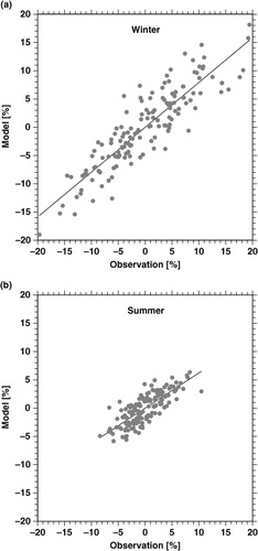
Figure 8 shows a relationship between modelled (by PWLT) and observed TO₃ monthly means. The scatter plots are for the season with the best (in winter) and the worst (in summer) model performance. Both modelled and observed TO₃ values in summer are much less variable than those in winter due to seasonal differences of the dynamical forcing on the ozone layer, for example, strong planetary wave activity and the Brewer–Dobson circulation in winter. The percent of the variance explained by the PWLT model, that is, the so-called R ² value (squared the correlation coefficient between the modelled and observed series), equals 79% in winter and 62% in summer. The model-observation agreement, as expressed by R ² value, is almost the same for all considered trend models. R ² values match those obtained in other trend studies, for example Nair (2012) found R ²=65% for the regression model applied to the year-round monthly TO₃ data taken by the Dobson spectrophotometer at Haute–Provence Observatory for the period 1984–2010.

Fig. 8 The modelled monthly deviations of total ozone relative to the long-term (1963–2012) means as a percent of the long-term mean versus those from the observations. (a) winter (DJF), (b) summer (JJA). The straight line shows the standard least squares fit to the data.

A zero trend line in the period 1963–1974 is assumed in the trend formula by EESC and PWLT models [eq. (4) and (5)] as the early ozone observations might be of lower accuracy. The first data validation of the Belsk's ozone was carried in summer 1974 during the international calibration campaign at Belsk. The FLEX trends in the early data appear statistically significant in winter and summer (Table 2). It cannot be excluded that such trends are due to instrument's calibration problems and should be treated with care. It seems that the long-term pattern of ozone changes in the early data has only a slight influence on the trends in subsequent years as the trend values are almost the same in the period 1975–1996 by all the considered trend models regardless of the assumed trend pattern in the early data.

Table 2 The trends by the examined trend models for the four seasons of the year and the year-round monthly total ozone values

Trend (% per decade)
	1963–1974	1975–1996			1997–2012
Data set	FLEX	EESC	PWLT	FLEX	EESC	PWLT	FLEX
Winter	−4.7 (2.6)	−4.2 (0.9)	−4.0 (1.1)	−3.1 (0.8)	1.4 (0.3)	0.8 (2.0)	−1.0 (1.6)
Spring	−0.4 (2.4)	−3.2 (0.8)	−3.1 (1.0)	−2.9 (0.7)	1.3 (0.3)	0.1 (1.6)	0.5 (1.5)
Summer	1.8 (1.4)	−2.0 (0.8)	−1.4 (0.5)	−1.8 (0.5)	0.7 (0.3)	−1.4 (0.5)	−0.5 (0.9)
Autumn	1.7 (1.8)	−1.7 (0.6)	−1.5 (0.7)	−1.5 (0.5)	0.6 (0.2)	−0.0 (1.2)	−0.3 (1.2)
Year	0.5 (1.7)	−2.7 (0.5)	−2.5 (0.5)	−2.2 (0.5)	0.9 (0.2)	0.1 (1.4)	−0.3 (1.0)

The trend errors at 2σ level are in the parentheses. The statistically significant results are in bold font.

Table 2 shows the trend values by the examined models for the period 1975–1996 and 1997–2012. The ozone trend in the former period is of about 2–3% per decade in the year-round data, 3–4% per decade in winter/spring seasons, and about 1.5–2% per decade in summer/autumn seasons. There are larger differences between the model results in the latter period. EESC model yields the positive trends in all seasons as a consequence of decreasing ODS concentration. PWLT model provides a statistically significant negative trend in summer (1.4% per decade) in the whole 1975–2012 period.

PWLT trends in the period 1975–1996 and 1997–2012 are the same for summer as the stepwise regression deleted the second term of the PWLT trend [i.e. γ =0 in eq. (5)]. A number of months with positive fractional TO₃ deviations appeared around 1980 in summer and the straight line fit for the whole period 1976–2012 is better than that by two joint lines with the turning point in 1997. The trend by FLEX model in the period 1997–2012 is not sensitive to the ozone values around 1980 and insignificant FLEX trend for that period suggests that statistically significant negative PWLT trend in the period 1997–2012 should be treated with care.

The FLEX trends in the period 1997–2012 are not statistically significant. All of the trends calculated by the considered models are within the range of about ±1.5% per decade. This means that there is no deepening of the ozone loss in the 1997–2012 period when compared to the ozone behaviour during the ODS increasing period in the stratosphere.

The spring trends in the Umkehr layers (Table 3) show the ozone depletion in the former period for the whole ozone column, for the lower (layer 2+3+4) and the upper (layer 7+8) stratospheric ozone. The trends calculated by EESC and FLEX models provide the trend overturning in these stratospheric regions, that is, the statistically significant (at 2σ level) positive trends since 1997 appearing after the negative ones before. In the former period for summer and autumn, the negative trends (by FLEX model) are found for TO₃ and ozone content in the upper stratosphere. In the later period for summer and autumn, the statistically significant negative trends are revealed by FLEX model in all considered layers except the upper stratosphere. The trend overturning is found for all seasons in the upper stratosphere and in the lower stratosphere only for the spring data. EESC and PWLT models sometimes show insignificant trends in the ozone profile, especially in summer and autumn (see NA values in Table 3). In these cases, the trend terms were excluded from the statistical model by the stepwise regression used to eliminate redundant regression terms.

Table 3. The same as Table 2 by the trends are for the ozone content in the selected combined Umkehr layers and for sum of the ozone content in all 10 layers (total ozone)

	Trend 1975–1996 (% per decade)			Trend 1997–2012 (% per decade)
Umkehr layer	EESC	PWLT	FLEX	EESC	PWLT	FLEX
Spring
All	−2.9 (1.0)	−3.1 (1.2)	−2.6 (0.8)	1.0 (0.4)	1.5 (2.0)	1.0 (1.8)
2+3+4	−3.6 (1.8)	−4.2 (2.1)	−3.2 (1.6)	1.3 (0.6)	3.0 (3.6)	2.8 (2.6)
5+6	NA	NA	−0.2 (0.7)	NA	NA	−1.0 (1.4)
7+8	−3.7 (2.0)	−4.5 (2.4)	−3.5 (1.2)	1.3 (0.7)	3.7 (3.9)	3.5 (2.5)
Summer
All	−0.6 (0.7)	−0.5 (0.4)	−0.7 (0.5)	0.2 (0.2)	−0.5 (0.4)	−1.1 (1.0)
2+3+4	NA	NA	−0.6 (1.0)	NA	NA	−1.8 (1.7)
5+6	NA	NA	−0.1 (0.6)	NA	−1.2 (1.3)	−1.9 (1.2)
7+8	NA	NA	−2.5 (1.2)	NA	NA	2.6 (2.5)
Autumn
All	NA	−0.5 (0.5)	−0.7 (0.5)	NA	−0.5 (0.5)	−1.2 (0.9)
2+3+4	NA	NA	0.3 (0.8)	NA	NA	−1.4 (1.2)
5+6	NA	NA	−0.1 (0.6)	NA	NA	−1.2 (1.1)
7+8	−1.5 (1.7)	−2.3 (2.1)	−2.6 (0.6)	0.6 (0.6)	3.0 (3.3)	1.9 (1.1)

The results of the statistical-simulation-based test concerning the trend overturning in 1997 and 2005 are shown in Table 4 (for TO₃) and Table 5 (for the ozone content in the Umkehr layers). The weakening of the TO₃ negative trend since 1997 is corroborated by the test results, with the exception of the autumn trends (but in this case 93.6% bootstrap simulations support the hypothesis, i.e. close to the 95% threshold). This hypothesis is also true for the column amount of ozone in the Umkehr days for spring. Surprisingly, it appears that the hypothesis of more negative TO₃ trend in the latter period comparing to that in the former period is true for the layer 5+6 (in summer) and for the layer 2+3+4 (in autumn). It is worth mentioning that the trends are based on the monthly means averaging limited number of the ozone daily profiles. Thus, such a monthly mean profile could differ from a hypothetical one based on all daily data in a month.

Table 4. The probability of appearance of the total ozone trend in the period 1997–2012 higher than that in the period 1975–1996 (Tr_75–96<Tr_97–12), the positive trends in the period 1997–2012 (Tr_97–12>0), 1997–2005 (Tr_97–05>0) and 2005–2012 (Tr_05–12>0)

Data set	Tr75–96<Tr97–12	Tr97–12>0	Tr97–05>0	Tr05–12>0
Winter	97.9	18.6	81.8	4.4
Spring	99.8	76.7	86.4	52.5
Summer	95.0	5.9	29.2	10.0
Autumn	93.6	35.7	35.4	43.8
Year	99.5	34.0	66.0	25.7

The probabilities are retrieved from 10000 bootstrap simulations for the four seasons of the year and for the year-round data. Statistically significant results are in bold font.

Table 5. The same as Table 4 but results are for the Umkehr total ozone and the ozone content in the joint neighbouring Umkehr layers: 2+3+4 – the lower stratosphere, 5+6 – the middle stratosphere, and 7+8 – the upper stratosphere

Data set	Tr75–96<Tr97–12	Tr97–12>0	Tr97–05>0	Tr05–12>0
Umkehr layers 1+ … +10 (total ozone)
Spring	99.8	86.3	83.4	69.0
Summer	25.6	1.5	62.1	1.2
Autumn	15.0	0.7	45.4	0.7
Umkehr layers 2+3+4
Spring	99.8	96.3	90.4	84.8
Summer	17.1	4.3	81.2	1.3
Autumn	4.1	3.5	27.4	5.3
Umkehr layers 5+6
Spring	20.8	9.1	83.4	2.7
Summer	4.8	0.9	65.8	0.5
Autumn	5.6	1.8	79.2	0.6
Umkehr layers 7+8
Spring	100.0	99.7	66.4	99.5
Summer	99.9	97.7	69.0	96.2
Autumn	100.0	99.8	83.7	99.6

The decline of TO₃ from the observations in the Umkehr days is disclosed in the latter period in summer and autumn. The probability of positive TO₃ trend in the period 1997–2012 is only 1.5% and 0.7% for summer and autumn, respectively (Table 5). The TO₃ decrease in the period 1997–2012 is due to the corresponding ozone decline in the lower stratosphere (layer 2+3+4, the probability of increasing ozone is 4.3% and 3.5% for summer and autumn, respectively) and in the mid-stratosphere (layer 5+6, the probability of increasing ozone is 0.9% and 1.8% for summer and autumn, respectively). The TO₃ decrease in summer since 1997 is also supported by the test applied to the TO₃ data collected during standard all-sky TO₃ measurements. Only 5.9% bootstrap simulations for summer show (Table 4) the TO₃ increase in the period 1997–2012. The summer/autumn decrease of TO₃ and the ozone amount in the lower and middle stratosphere in the latter period are mostly due to the ozone decline in the period 2005–2012 as the probabilities below the 5% threshold do not appear in the period 1997–2005 (Table 5).

5. Discussion and conclusion

All of the examined models show statistically significant negative TO₃ trends in the period 1975–1996 for the four seasons of the year and for the whole year with the stronger depletion in the winter/spring season comparing to that in the summer/autumn season. A slowing of the downward trend is the common feature of the trend pattern by the analysed models for the period 1997–2012. Thus, according to the WMO classification (WMO, 2007), the first step of the ozone recovery could be announced. EESC model shows statistically significant upward trend in the latter period related to the ODS decreasing trend. Thus, the next stage of the ozone recovery could be announced, but it is not corroborated by results of PWLT and FLEX models. The trend components by these models are not only exclusively linked to ODS changes but could also contain a signal due to other unknown, yet long-term forcing on the ozone layer.

Analysis of the long-term ozone variability by the triad trend model has been proposed by Krzyścin and Rajewska-Więch (2009). Their analyses of the Belsk's TO₃ data based on the Dobson measurements for the period 1963–2008 showed a similar picture of the ozone changes and the differences between the models. All models disclosed the first stage of the ozone recovery. The second stage was supported only by EESC model. Nevertheless, the updated TO₃ series does not show a convincing signal of the positive ozone trend since the TO₃ minimum in the mid-1990s. Krzyścin (2012) analysing the global ground-based TO₃ data by the triad trend model found such signal in the zonal TO₃ means for the 50°S–50°N region (in summer and in the entire year) and for the whole globe (in spring) in the period 1996–2008.

The Umkehr observations are carried out in cloudless periods a few hours after sunrise or before sunset. The profile trend analyses by EESC and FLEX model reveal the second stage of the recovery during spring for the lower stratosphere (Umkehr layer 2+3+4) and for the upper stratosphere (Umkehr layer 7+8). In addition, FLEX model also provides the second stage of the recovery for the upper stratospheric ozone in summer and autumn.

The trend analyses of the summer and autumn Umkehr profiles (Table 3) show statistically significant negative trends (by FLEX model) in the whole column and for the lower and mid-stratosphere region in the period 1997–2012. Tests concerning sign of the trend values reveal that this decline is mostly due to the ozone decline since about 2005 (Table 5). Such a trend behaviour could have a serious health consequence as the ozone decline appears in summer during fine weather conditions allowing the Umkehr observations, that is, in days when the natural UV level is high and outdoor activity is more frequent.

Recent studies have been focused on the analyses of the long-term ozone variability and its dependence on the man-made changes in the ODS level in the mid-altitude stratosphere. Determination of the stage of the stratospheric ozone recovery was the key point of these studies (e.g. Steinbrecht et al., 2004; Zanis et al., 2006; Fioletov, 2008; Vigouroux et al., 2008; Angell and Free, 2009; Krzyścin, 2012, Nair, 2012). There is no doubt that a weakening of the negative ozone trend appeared since the mid-1990s, that is, the first stage of the ozone recovery could be announced in the extratropical regions (e.g. Miller et al., 2006; Mäder et al., 2010; WMO, 2011). This finding also provides evidence for the effectiveness of MP for the protection of the ozone layer. The second stage of the recovery (the trend overturning) has been documented for the zonally averaged TO₃ data for Antarctica (Salby et al., 2011; Kuttippurath et al., 2013), NH regions up to 50°N (see Fig. 2.3 of WMO, 2011), 50°S–50°N region, and the whole globe (Krzyścin, 2012).

Recent trend analyses of the individual station data were not conclusive about the recovery stage of the NH ozone. For example, there were no statistically significant trends over the Jungfraujoch (47°N) in the period 1995–2009 over the low-, mid- and upper stratosphere and in TO₃ (WMO, 2011, see Table 2–1 updated from Vigouroux et al., 2008). Whereas the statistically significant trend was found over Harestua (60°N); negative in the lower stratosphere, positive in the mid- and upper stratosphere, but not statistically significant TO₃ trend. Recent trend analysis of total and profile ozone and for Haute-Provence Observatory (44°N) supports the second stage of ozone recovery based on positive trend values in TO₃, in the ozone content in the lower and upper stratosphere in the period 1997–2010, Nair (2012). Umkehr data for Arosa show that the negative trends in the period 1970–1995 and the positive trend appeared during 1996–2004 only above 33 km (Zanis et al., 2006).

The Belsk's ozone profiles show that the second stage of recovery could be claimed for the upper stratospheric level (Umkehr layer 7+8) in spring/summer/autumn data and for the lower stratosphere (Umkehr layer 2+3+4) only in spring. Surprisingly, continuation of the TO₃ depletion is found in the Belsk's Umkehr data (by FLEX model) for summer and autumn in the period 1997–2012. Such a decline is due to the ozone decrease both in the lower stratosphere and mid-stratosphere found during clear-sky conditions (the Umkehr days).

The TO₃ decreasing tendency could also be revealed at the Belsk's neighbouring station, Hradec Kralove (49°N), during fine weather conditions in the period 1994–2010 (Vaniček et al., 2012, see their Table 2). Based on the reconstructed TO₃ data (since 1950), Krzyścin and Borkowski (2008) found that the negative trends were also possible over small areas in Europe before the period of significant man-made impact on the ozone layer. The long-term analysis should be applied both to the monthly means and various subsets of the ozone monthly data. Such an approach has also been suggested in a recent paper by Rieder et al. (2011, 2013) focusing on the distribution of the ozone monthly extrema (minima and maxima) and their relationship with the known dynamical regressors.

A slight positive trend in the NH midlatitudinal ozone is expected from the mid-1990s due to the ODS level decrease. Results of FLEX model suggest that it seems possible that unknown processes have already started to influence the ozone variability at Belsk in recent years. Moreover, the current trend models only use the linear combination of the dynamical proxies (e.g. Mäder et al., 2007) to explain the dynamical part of the ozone variability but nonlinear dynamical effects and interactions between the dynamical and chemical processes may be important for the trend detection. Evidently, there is a need for further monitoring and analyses of the ozone variability.

6. Acknowledgements

This work is partially supported by the National Science Centre grant no. UMO-2011/01/B/ST10/06892. The authors thank two anonymous reviewers for their valuable comments, which helped them to improve this article.

References

- Angell J. K , Free M . Ground-based observations of the slowdown in ozone decline and onset of ozone increase. J. Geophys. Res. 2009; 114 D07303, 1–9.
- Chubachi S . Preliminary result of ozone observations at Syowa station from February 1982 to January 1983. Mem. Natl. Inst. Polar Res. Spec. Issue Jpn. 1984; 34: 13–20.
- Cleveland W. S . Robust locally weighted regression and smoothing scatterplots. J. Am. Stat. Assoc. 1979; 74(368): 829–846.
- Crutzen P . A discussion of the chemistry of some minor constituents in the stratosphere and troposphere. Pure Appl. Geophys. 1973. 106–108(1), 1385–1399.
- Degórska M , Krzyścin J , Rajewska-Więch R , Bojkov R. D , Fabian P . Ozone trends from Dobson station at Belsk, Poland, Ozone in the Atmosphere. Proceedings of the Quadrennial Ozone Symposium 1988 and Tropospheric Ozone Workshop, 4–13 August, 1988 in Göttingen, FRG. 1989; Hampton, VA: A. Deepak Publishing. 120–123.
- Degórska M , Rajewska-Więch B . Retrospective reevaluation of total ozone and Umkehr profile data from Belsk, Poland. Publ. Inst. Geophys. Pol. Acad. Sci. D. 1991; 36(246): 71–76.
- Degórska M , Rajewska-Więch B , Krzyścin J . Reduction of variance of total ozone and Umkehr profiles after re-evaluation of the Belsk records. Publ. Inst. Geophys. Pol. Acad. Sci. D. 1995; 42(269): 91–101.
- Dobson G. M. B . Observers’ handbook for the ozone spectrophotometer. Ann. Int. Geophys. Year. 1957; V(1): 46–89.
- Dziewulska-Łosiowa A , Degórska M , Rajewska-Więch B . The normalized total ozone data record, Belsk, 1963–1983. Publ. Inst. Geophys. Pol. Acad. Sci. D. 1983; 18(169): 23–73.
- Farman J. C , Gardiner B. G , Shanklin J. D . Large losses of total ozone in Antarctica reveal seasonal ClO X/NO X interaction. Nature. 1985; 315: 207–210.
- Fioletov V. E . Ozone climatology, trends, and substances that control ozone. Atmos. Ocean. 2008; 46(1): 39–67.
- Fioletov V. E , Shepard T. G . Summertime ozone variations over middle and polar latitudes. Geophys. Res. Lett. 2005; 32 L04807, 1–5.
- Fioletov V. E , Tarasick D. W , Petropavlovskikh I . Estimating ozone variability and instrument uncertainties from SBUV (/2), ozonesonde, Umkehr, and SAGE II measurements: short-term variations. J. Geophys. Res. 2006; 111 D02305, 1–14.
- Harris J. M , Oltmans S. J , Tans P. P , Evans R. D , Quincy D. L . A new method for describing long-term changes in total ozone. Geophys. Res. Lett. 2001; 28(24): 4535–4538.
- Harris N. R. P , Kyrö E , Staehelin J , Brunner D , Andersen S.-B , co-authors . Ozone trends at northern mid- and high latitudes – a European perspective. Ann. Geophys. 2008; 26(5): 1207–1220.
- Johnston H. S . Reduction of stratospheric ozone by nitrogen oxide catalysts from supersonic transport exhaust. Science. 1971; 173: 517–522.
- Krzyścin J . Change in ozone depletion rates beginning in the mid 1990s: trend analyses of the TOMS/SBUV merged total ozone data, 1978–2003. Ann. Geophys. 2006; 24: 493–502.
- Krzyścin J , Rajewska-Więch B . Ozone recovery as seen in perspective of the Dobson spectrophotometer measurements at Belsk (52°N, 21°E) in the period 1963–2008. Atmos. Environ. 2009; 43(40): 6369–6375.
- Krzyścin J. W . Onset of the total ozone increase based on statistical analyses of global ground-based data for the period 1964–2008. Int. J. Clim. 2012; 32(2): 240–246.
- Krzyścin J. W , Borkowski J. L . Variability of the total ozone trend over Europe for the period 1950–2004 derived from reconstructed data. Atmos. Chem. Phys. 2008; 8(11): 2847–2857.
- Krzyścin J. W , Jaroslławski J , Rajewska-Więch B . Beginning of the ozone recovery over Europe? – analysis of the total ozone data from the ground-based observations, 1964–2004. Ann. Geophys. 2005; 23: 1–11.
- Kuttippurath J , Lefèvre F , Pommereau J.-P , Roscoe H. K , Goutail F , co-authors . Antarctic ozone loss in 1989–2010: evidence for ozone recovery?. Atmos. Chem. Phys. Discuss. 2013; 13: 1625–1635.
- Mäder J. A , Staehelin J , Brunner D , Stahel W. A , Wohltmann I , co-authors . Statistical modeling of total ozone: selection of appropriate explanatory variables. J. Geophys. Res. 2007; 112 D11108.
- Mäder J. A , Staehelin J , Peter T , Brunner D , Rieder H. E , co-authors . Evidence for the effectiveness of the Montreal Protocol to protect the ozone layer. Atmos. Chem. Phys. 2010; 10: 12161–12171.
- Mateer C. L , DeLuisi J. J . A new Umkehr inversion algorithm. J. Atmos. Terr. Phys. 1992; 54: 537–556.
- Miller A. J , Cai C , Tiao G , Wuebbles D. J , Flynn L. E , co-authors . Examination of ozonesonde data for trends and trend changes incorporating solar and Arctic oscillation signals. J. Geophys. Res. 2006; 111 D13305, 1–10.
- Molina M. J , Rowland F. S . Stratospheric sink for chlorofluoromethanes: chlorine atom-catalysed destruction of ozone. Nature. 1974; 249: 810–812.
- Nair P. J . Evolution of Stratospheric Ozone in the Mid-Latitudes in Connection with the Abundances of Halogen Compounds. 2012. PhD Thesis. University of Pierre and Marie Curie – Paris V, Online at: http://tel.archives-ouvertes.fr/docs/00/73/35/55/PDF/02-GOPALAPILLAI-memoire.pdf .
- Newman P. A , Daniel J. S , Waugh D. W , Nash E. R . A new formulation of equivalent effective stratospheric chlorine (EESC). Atmos. Chem. Phys. 2007; 7: 4537–4552.
- Petropavlovskikh I , Bhartia P. K , DeLuisi J . New Umkehr ozone profile retrieval algorithm optimized for climatological studies. Geophys. Res. Lett. 2005; 32 L16808, 1–5..
- Petropavlovskikh I , Evans R. D , Carbaugh G. L , Maillard E , Stubi R . Towards a Better Knowledge of Umkehr Measurements: A Detailed Study of Data from Thirteen Dobson Intercomparisons. 2008. Global Atmospheric Watch (GAW) No. 180, WMO/TD-No. 1456, WMO, Geneva, Switzerland, 46 pp..
- Rajewska-Więch B , Bialek M , Krzyścin J. W . Quality control of Belsk's Dobson spectrophotometer: comparison with the European sub-standard Dobson spectrophotometer and satellite (OMI) overpasses. Publ. Inst. Geophys. Pol. Acad. Sci. D. 2006; 67(382): 115–121.
- Reinsel G. C , Miller A. J , Weatherhead E. C , Flynn L. E , Nagatani R. M , co-authors . Trend analysis of total ozone data for turnaround and dynamical contributions. J. Geophys. Res. 2005; 110 D16306, 1–14.
- Rieder H. E , Frossard L , Ribatet M , Staehelin J , Maeder J. A , co-authors . On the relationship between total ozone and atmospheric dynamics and chemistry at mid-latitudes – part 2: the effects of the El Niño/Southern Oscillation, volcanic eruptions and contributions of atmospheric dynamics and chemistry to long-term total ozone changes. Atmos. Chem. Phys. 2013; 13: 165–179.
- Rieder H. E , Jancso L. M , Di Rocco S , Staehelin J , Mäder J. A , co-authors . Extreme events in total ozone over the Northern mid-latitudes: an analysis based on long-term data sets from five European ground-based stations. Tellus. B. 2011; 63(5): 860–874.
- Salby M , Titova E , Deschamps L . Rebound of Antarctic ozone. Geophys. Res. Lett. 2011; 38: L09702.
- Steinbrecht W , Claude H , Winkler P . Reply to comment by D. M. Cunnold et al. on “enhanced upper stratospheric ozone: sign of recovery or solar cycle effect?”. J. Geophys. Res. 2004; 109 D14306, 1–4.
- Storch H. V , Zwiers F. W . Statistical Analysis in Climate Research: Fitting Statistical Model. 1999; Cambridge, UK: Cambridge University Press. 499.
- Stratospheric Processes and their Role in Climate (SPARC). Assessment of Trends in the Vertical Distribution of Ozone 1998. 1998; 416. SPARC Report No. 1, WMO Ozone Research and Monitoring Project Report No. 43, World Climate Research Programme, Geneva.
- Vaniček K , Metelka L , Skřivánková P , Stanék M . Dobson, Brewer, ERA-40 and ERA-interim original and merged total ozone data sets –evaluation of differences: a case study, Hrádec Kralové (Czech), 1961–2010. Earth Syst. Sci. Data. 2012; 4: 91–100.
- Vigouroux C , De Mazière M , Demoulin P , Servais C , Hase F , co-authors . Evaluation of tropospheric and stratospheric ozone trends over Western Europe from ground-based FTIR network observations. Atmos. Chem. Phys. 2008; 8: 6865–6886.
- Vyushin D , Fioletov V. E , Shepherd T. G . Impact of long-range correlations on trend detection in total ozone. J. Geophys. Res. 2007; 112: 1–18.
- Weatherhead E. C , Reinsel G. C , Tiao G. C , Meng X.-L , Choi D , co-authors . Factors affecting the detection of trends: statistical considerations and applications to environmental data. J. Atmos. Res. 1998; 103: 17149–17161.
- Wohltmann I , Lehmann R , Rex M , Brunner D , Mäder J . A process-oriented regression model for column ozone. J. Geophys. Res. 2007; 112 D12304, 1–18.
- World Meteorological Organization (WMO). International Ozone Trends Panel Report 1988. 1989; 817. Global Ozone Research and Monitoring Project Report No. 18, WMO, Geneva, Switzerland.
- World Meteorological Organization (WMO). Report of WMO/NOAA meetings on ozone data re-evaluation and use of Dobsons and Brewers in the G030S. Proceedings of the Fourth WMO/NOAA Workshop on Ozone Data Re-Evaluation. 1996; 59. Global Ozone Research and Monitoring Project Report No. 36, WMO, Geneva, Switzerland.
- World Meteorological Organization (WMO). Scientific Assessment of Ozone Depletion: 2006. 2007; 572. Global Ozone Research and Monitoring Project – Report No. 50, WMO, Geneva, Switzerland.
- World Meteorological Organization (WMO). Scientific Assessment of Ozone Depletion: 2010. 2011; 516. Global Ozone Research and Monitoring Project – Report No. 52, WMO, Geneva, Switzerland.
- Yang S.-K , Long C. S , Miller A. J , He X , Yang Y , co-authors . Modulation of natural variability on a trend analysis of updated cohesive SBUV(/2) total ozone. Int. J. Rem. Sens. 2009; 30(15): 3975–3986.
- Zanis P , Maillard E , Staehelin J , Zerefos C , Kosmides E , co-authors . On the turnaround of stratospheric ozone trends deduced from the reevaluated Umkehr record of Arosa, Switzerland. J. Geophys. Res. 2006; 111 D22307, 1–15.