Influence of coastal upwelling on the air–sea gas exchange of CO₂ in a Baltic Sea Basin

Abstract

During coastal upwelling cold water from the ocean interior with high CO₂ concentration is brought up to the surface, allowing this water to interact with the atmosphere. This sets the stage for events with potentially altered sea–air CO₂ fluxes. Four upwelling events off the east coast of Gotland in the Baltic Sea were analyzed to assess the impact of upwelling on the air–sea exchange of CO₂. For each event, the observed pCO₂ were found to be a function of sea-surface temperature (SST) in the upwelling area, which allowed satellite observations of SST to form a proxy for surface water pCO₂. A bulk formula was then used to estimate the air–sea CO₂ flux during the upwelling events. The results show that the CO₂ fluxes in the study area are highly influenced by the upwelling. Comparing with idealized cases without upwelling yields relatively large differences, ranging between 19 and 250% in reduced uptake/increased emission of CO₂. Upwelling may also influence the CO₂ fluxes on larger scales. A rough estimate indicates that it may also be of significant importance for the average annual CO₂ flux from the Baltic Sea. Including upwelling possibly decreases the Baltic Sea annual average uptake by up to 25%.

• coastal upwelling
• carbon dioxide
• air–sea exchange
• Baltic Sea measurements
• remote sensing

1. Introduction

Upwelling is a commonly observed phenomenon along coastlines where wind-driven horizontal divergence in the sea can cause cold, nutrient-rich water from below or within the thermocline, to rise to the surface. When the wind blows parallel to the coast with the coast on the left-hand side (on the northern hemisphere), surface water is transported away from the coast due to the effect of the Coriolis force. To replace the removed surface water, water is brought up to the surface from below. In the semi-enclosed Baltic Sea, coastal upwelling can be as frequent 25–30% of the time in some areas (Gidhagen, 1987; Lehmann et al., 2012). Signatures of upwelling are generally observed from spring to autumn when there is a strong thermal stratification with warm surface water and colder water below. The typical upwelling event in the Baltic Sea has a vertical motion of 10⁻⁵–10⁻⁴ m s⁻¹ or 1–10 m day⁻¹ (Hela, 1976), a horizontal scale of 10–20 km offshore and 100 km alongshore (Gidhagen, 1987); a typical temperature change of 1–5°C day⁻¹ (Hela, 1976); a horizontal temperature gradient of 1–5°C km⁻¹ (Krężel et al., 2005); and a lifetime from a few days to 1 month (Lehmann and Myrberg, 2008). Since coastal upwelling is triggered by winds parallel to the coast, the frequency of upwelling in different regions in the Baltic Sea varies with the prevailing wind direction. When easterly winds prevail, the Estonian coast of the Gulf of Finland, the Polish and the German coasts have a high frequency of upwelling; when northerly winds prevail, the eastern Baltic coast, and the eastern coast of Bothnian Bay have a high frequency; and when south- and south-westerly winds prevail, the Finnish coast of the Gulf of Finland, the southern Swedish coast, the western coast of Bothnian Bay, and the southeast coast of Gotland have a high frequency (Lehmann et al., 2012).

An important effect of upwelling is the transport of water masses with relatively high CO₂ concentration from the ocean interior to the sea surface. This alters the surface water CO₂ concentration influencing the air–sea CO₂ fluxes. A recent example is the study by Mathis et al. (2012) which estimates that sea–air CO₂ fluxes during upwelling, on the Beaufort shelf in the western Arctic Ocean, are of similar magnitude as the total annual sink of CO₂ in the Beaufort Sea. Thus, due to the frequent occurrence of upwelling in the Baltic Sea, this process has the possibility to significantly alter the net CO₂ uptake/release of CO₂ by the surface water in this region. Current estimates of the net uptake/release of CO₂ of the Baltic Sea are ambiguous, some sub-basins acts as sources of atmospheric CO₂, whereas others acts as sinks (Thomas and Schneider, 1999; Algesten et al., 2006; Kuss et al., 2006; Omstedt et al., 2009; Wesslander et al., 2010; Kulinski and Pempkowiak, 2012; Löffler et al., 2012; Norman et al., 2013). Three of these previous studies included the entire Baltic Sea in the budget calculations: Omstedt et al. (2009), Kulinski and Pempkowiak (2012) and Norman et al. (2013) none of which considered the influence of upwelling. The modelling results in Omstedt et al. (2009) showed that prior to the industrial revolution, the Baltic Sea was a source of CO₂, and at this present time the sea alters between being a source and a sink during different parts of the year. The results in Norman et al. (2013), using the same model as in Omstedt et al. (2009), indicated that the Baltic Sea acts as a net sink of 0.22 mol CO₂ m⁻² yr⁻¹. However, Kulinski and Pempkowiak (2012) concluded that the Baltic Sea acts as a net source of 0.25 mol CO₂ m⁻² yr⁻¹, using a somewhat different approach. Including upwelling in the estimates has the potential to significantly alter these numbers.

In this study, we combine the surface measurements at the Östergarnsholm site with satellite remote sensing of sea-surface temperature (SST) to study the effects of upwelling on the air–sea CO₂ fluxes in the region. The methods used for flux estimations are described in Section 2. In Section 3, the in situ measurements and satellite data are described. The results are presented in Section 4, discussion in Section 5, and summary and conclusions are presented in Section 6.

2. In situ measurements and remote sensing

2.1. The Östergarnsholm site

The measurement site has been running since 1995, and it is located on the small island Östergarnsholm in the central Baltic Sea, 4 km from the east coast of Gotland (Fig. 1). A 30-m-high tower, with its base approximately 1 m above sea level, is instrumented at various heights and situated at (57.42°N, 18.99°E) on the southernmost tip of the flat island. Gill sonic anemometers are positioned at three levels (9, 16.5 and 25 m above the tower base) and LICOR LI-7500 at two levels (9 and 25 m above the tower base). The LICOR LI-7500, an open-path infrared gas analyzer, is used in combination with the sonic anemometer to measure fluxes of CO₂ and water vapour. Slow-response measurements of temperature are made using ventilated and radiation-shielded copper-constant thermocouples at five levels (6.9, 11.9, 14.3, 20.2 and 28.8 m above the tower base). Slow-response measurements of air pressure and relative humidity are measured at 1 and 8 m, respectively. At 9 m above the tower base, an infrared gas analyzer (IRGA, PP-systems) measures CO₂ in the atmosphere with a 30-minute time resolution. SST and pCO_2w is measured by a SAMI-CO₂ sensor (Submersible Autonomous Moored Instrument). The SAMI is located at 4 m depth, 1 km southeast from the tower (Fig. 1) and is in use semi-continuously. In addition, SST is also measured by a wave rider buoy (operated by the Finnish Meteorological Institute) at 0.5 m depth about 4 km southeast of the tower (Fig. 1).

Fig. 1 Map of the Baltic Sea and Östergarnsholm site showing the position of the meteorological tower, the SAMI-sensor, and the Wave rider buoy (from Rutgersson et al., 2008).

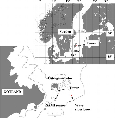
The footprint area, the upwind surface from which the measured flux originates, was calculated in Högström et al. (2008) for the Östergarnsholm site. The flux footprint was estimated for different measurement heights and different stratifications. An average value based on neutral, stable and unstable cases was calculated which showed that for measurements at 10 m height, 50% of the fluxes originate from an area within 760 m, while 80% of the fluxes originate from a distance within 2900 m from the tower. For the 26 m measurement height, the corresponding values are 2900 and 12 000 m. The geometrical area of the footprint, from where the majority of the flux originates, is 0.6 km² for measurement height 10 m and 6.2 km² for 26 m height.

Furthermore, the tower measurements at the Östergarnsholm site represent open-sea conditions when the wind direction is 80–210° (Högström et al., 2008), although Rutgersson et al. (2008) showed that the SAMI sensor represents the footprint of the tower only for wind directions 80–160°. Hence, the SAMI sensor might not represent surface measurements for wind directions >160° as the horizontal heterogeneity could be significantly closer to the coast. This is of major importance during the summer months when the biological activity is large close to the coast of Gotland, and during upwelling events.

For the flux estimations in this study, some restrictions of the data are made to include only high-quality measurements in the analysis. When the wind speed is <2 m s⁻¹, the data are dominated by noise and rejected. The LI-7500 gas analyzer is sensitive to condensation on the analyzer window, and hence data indicating a relative humidity >95% are not used. Furthermore, a quality control of the CO₂ measurements is performed manually by inspecting the individual 30-minutes spectra. If the shape of the w- or CO₂-spectrum significantly deviates from the theoretical shape (Kaimal et al., 1972) with the result that the influence of the co-spectrum is considerable, the data are rejected. Moreover, data when the wind direction is 80–220° are selected for the analysis. The wind section 210–220° might be somewhat influenced by Gotland and not entirely representative of open-sea conditions, although it is included in the analysis since the wind direction during upwelling is generally south to southwest, and excluding data with wind direction 210–220° would exclude a majority of the upwelling cases.

This study is focused on four upwelling events with various lengths, from 8 to 17 d: 15–31 July 2005 (Period 1), 13–22 July 2007 (Period 2), 5–14 October 2008 (Period 3) and 24–31 October 2008 (Period 4). These periods are selected since data in the atmosphere as well as in the water were available during most of the periods. The upwelling events are identified from the measurements when the wind direction is south to southwest, the SST decreases rapidly, and the pCO_2w increases. During part of Period 1, atmospheric data are missing, and hence wind measurements from the Swedish Meteorological and Hydrological Institute (SMHI) meteorological station on Östergarnsholm are used. This station is located approximately 1 km north of the flux tower, and the measurement height is 10 m. The wind at the SMHI station is measured with a Vaisala wind vane and cup anemometer, and the data are available every third hour as a 10-minute average.

2.2. Satellite data

The daily satellite SST data for the period 2005–2008 are from the Advanced Very High Resolution Radiometer (AVHRR), on board the National Oceanic and Atmospheric Administration (NOAA) satellites. The AVHRR operates in five spectral bands: 0.6–0.7, 0.75–1.1, 3.5–4, 10.3–11.3, 1.5–12.5 µm. The German Federal Maritime and Hydrographic Agency Hamburg processed the raw data from two satellites using the TeraScan software (Siegel et al., 1994). The algorithm identifies and eliminates pixels with small clouds. Additionally, as radiometers measure in infrared channels, and thick clouds are opaque for infrared wavelengths, the occurrence of thick clouds reduces the amount of SST data.

A combination of factors, for example, Quality control in the standard satellite algorithm, small basin size and contamination from cloud and land, results in gaps in satellite SST over the Eastern Gotland Basin. As the objective of this study is to quantify the nature of CO₂ fluxes off the coast of Gotland during upwelling, an optimal spatial coverage is needed to map the areal extent of upwelling. Hence, a gap-filling technique is applied to provide maximum spatial coverage. Two gap-filling methods were tested. Method 1 is based on ‘nearest-neighbour-in-time’, and Method 2 applies linear interpolation. Applying Method 1, the pixel where SST is unavailable at a given time point, is filled with its ‘nearest-neighbour-in-time’. All pixels in the satellite data have SST values for at least some, if not at all, time points. Hence, when data are missing, the missing value is replaced with an SST value closest in time. For example: a given pixel has three time points missing (i.e. Day 2, Day 3 and Day 4). For Day 2, the pixel is filled with SST from Day 1, while Day 4 is filled with Day-5 SST. Day 3 will in this case be filled with an average of SST from Day 1 and Day 5, since the distance to those time points is equal. Using Method 2, a simple linear interpolation in time was applied to the satellite data. To avoid muting the spatial heterogeneity, none of the applied gap-filling methods are applied in latitude or longitude. The difference between the two gap-filling techniques was mainly found in the amount of filled gaps, as Method 2 does not extrapolate at the boundaries. In this study, the gap-filling method which fills the largest amount of gaps is used, namely Method 1 which applies ‘nearest-neighbour-in-time’.

By interpolating over time instead of space, the heterogeneous pattern of upwelling is preserved. The effect of upwelling might, however, be under- or overestimated due to the interpolation. If the numbers of interpolated values are high in the upwelling region, it will significantly affect the estimated flux if the interpolated value differs considerably from the real value. This is of major importance during cases when the SST is strongly variable over time.

2.2.1. Upwelling detection method.

Upwelling events are identified from the in situ measurements of SST, pCO₂ and winds at Östergarnsholm. To quantify the area of upwelling, a detection method is applied to the satellite data. The detection method uses SST anomaly (SSTA) and distance from the coast as constraining parameters, and it is broadly based on the method developed by Lehmann et al. (2012). In Lehmann et al. (2012), the SSTA was calculated as the difference between the meridional average value of SST across the Baltic Sea and SST at each grid point. If SSTA is greater than 2°C within 20 km from the coast, the criteria for upwelling are fulfilled. Lehmann et al. (2012) used weekly data, and we found that their method was not optimal for data with daily time resolution. The upwelling detection method in this study is therefore modified as follows: an initial SST value, SST₀, is chosen as a day before the upwelling event starts. The SSTA at each grid point is SST₀ minus SST. From a sensitivity test, we found that using SSTA greater than 1°C within a distance of 50 km from the coast, the upwelling area was sufficiently captured, and consequently these criteria are applied.

3. Flux estimation methods

3.1. Bulk estimated fluxes

The air–sea exchange of gases is mainly controlled by the difference in partial pressure between the water surface and atmosphere, and the solubility of the gas in seawater, which depends on salinity and SST. Furthermore, various physical conditions and processes such as bubbles, sea spray, sea state, and water-side convection, determine the rate at which gases are exchanged over the air–sea interface (Wanninkhof et al., 2009; Rutgersson and Smedman, 2010; Rutgersson et al., 2011). The exchange rate is often referred to as the transfer velocity. The flux of CO₂, F _c , can hence be calculated as:1

where k is the transfer velocity, K ₀ the solubility, and ΔpCO₂ the difference of pCO₂ between water and air. As the wind is the driving force behind many of the processes controlling the transfer velocity, many parameterizations are based on wind speed square or cubic. The most commonly used parameterization is described by Wanninkhof (1992). Another parameterization, based on a larger data set than Wanninkhof (1992), is the empirical formulation by Nightingale et al. (2000):2

where u is the mean wind speed. Sc is the dimensionless Schmidt number (the ratio of kinetic viscosity of water and the diffusion coefficient of the gas), which is a function of SST and salinity, and 660 is the Schmidt number in seawater at 20°C. In eq. (2), k has the unit cm h⁻¹.

3.2. Measured fluxes using the eddy-covariance method

The eddy-covariance method is a direct method to estimate fluxes from high-frequency data (Aubinet et al., 2012). The flux of CO₂ is expressed as:3

where w (m s⁻¹) is the vertical wind component and ρ _c is the mass density of CO₂ (kg m⁻³). The overbar denotes a mean, and the prime a perturbation from the mean. The first term corresponds to the turbulent part of the flux, while the second term is related to the mean vertical motions.

The CO₂ density fluctuations measured by the open-path gas analyzer are influenced by simultaneous fluctuations of temperature and water vapour. This is often corrected for in the post-processing using the Webb–Pearman–Leuning correction (Webb et al., 1980). Alternatively, the direct conversion method developed by Sahlée et al. (2008) can be used. Applying the direct conversion method, the high-frequency time series is converted into a mixing ratio before the flux calculation. The flux of CO₂ is then derived as:4

where c is the mixing ratio of CO₂ and ρ _d the mass density of dry air (kg m⁻³). The direct conversion method is applied to the high-frequency atmospheric data of CO₂ in this study.

4. Results

4.1. Description of the upwelling events

The general features of the upwelling events along the east coast of Gotland are shown using mainly two representative periods which are described in more detail, Period 1 (15–31 July 2005) and Period 4 (24–31 October 2008).

The prevailing wind at the Östergarnsholm site during Period 1 is initially northwesterly, and thereafter becomes south-westerly, and parallel to the coast of Gotland (Fig. 2a). The upwelling is intermittent during the entire period, as the wind speed and direction vary (Fig. 2a and b). Wind directions parallel to the coast trigger upwelling, which result in decreasing SST (Fig. 2c). As the colder water reaches the surface, it starts to mix with the warmer surrounding water, and during wind directions not parallel to the coast, the SST increases since colder water is no longer lifted to the surface. Furthermore, to detect signatures of upwelling, the wind must be strong enough to force water to reach the surface from within or beneath the thermocline.

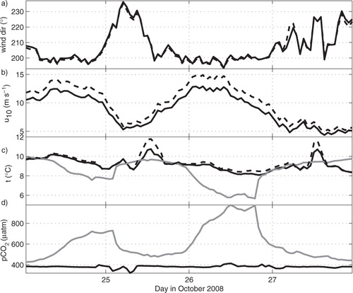
Fig. 2 Measurements at the Östergarnsholm site during Period 1: (a) wind direction (°); (b) wind speed (m s⁻¹); (c) air temperature (black solid line), water temperature from the SAMI sensor (grey solid line) and the wave rider buoy (grey dashed line) (°C); (d) pCO₂ in air (black solid line) and in water from the SAMI sensor (grey solid line) (µatm). The grey shaded area in (a) shows the wind direction 195°–225°, that is, the orientation of the southeastern part of the Gotland coastline.

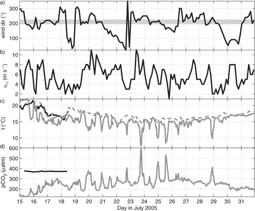
In the beginning of Period 1, the atmospheric stratification is unstable, that is, the sea surface is warmer than the air (Fig. 2c). As upwelling begins, SST at the site falls rapidly from 22 to 16°C in 5 hours, while the air temperature does not cool as rapidly. Hence, the atmosphere becomes more stably stratified during the upwelling event. Additionally, the SST is also measured 4 km east of the Östergarnsholm site at the Wave rider buoy (Fig. 1). At the beginning of Period 1, SST measured by the SAMI sensor and the Wave rider buoy have the same magnitude. However, the effect of upwelling is detected approximately 1 d later by the Wave rider buoy. Furthermore, the temperature at the Wave rider buoy does not decrease to the same low temperature as at the SAMI sensor. SST measured by the Wave rider buoy does not drop below 14°C, while the SST measured by the SAMI sensor dropped to 7°C on 23 July (Fig. 2c). We may speculate that the discrepancy is most likely due to horizontal heterogeneity, as the effect of upwelling is strongest close to the coast. The cold upwelled water is likely somewhat mixed with warmer water before it reaches the wave rider buoy. The atmospheric pCO₂ (pCO_2a) is relatively constant compared to sea-surface pCO₂ (pCO_2w), and we can assume that it is stay close to constant throughout the period. During the part of Period 1, when atmospheric measurements are available, pCO_2a has a magnitude of 368–396 µatm, and there is no obvious effect of upwelling on pCO_2a (Fig. 2d). The effect of upwelling is evident from the time series of pCO_2w. At the beginning of the period, pCO_2w has a value of 130 µatm, and the value increases intermittently (concurrent with SST decrease) during the period, with the highest value of 602 µatm on 23 July (Fig. 2d).

Although only of few days in the beginning of Period 1 have available atmospheric data, the study of Period 1 is relevant. It is a period of intermittent upwelling events, and the coverage of satellite data is good. Period 2 (13–22 July 2005) is also a period with intermittent upwelling due to variation in wind speed and direction. The effect of upwelling is, however, not as strong in Period 2 as in Period 1, as the SST decreases and the pCO_2w increase is less pronounced during Period 2.

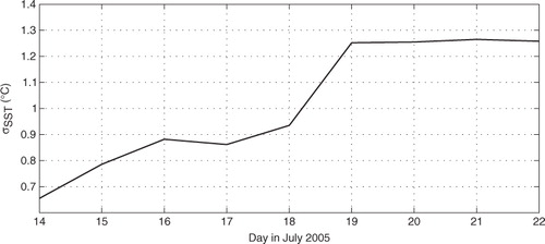
The horizontal extension and the evolution of upwelling during the beginning of Period 1 are shown in satellite images of SST (Fig. 3). On 14 July, the satellite image shows a homogenous picture, with SST values of 21–22°C in the entire area surrounding Gotland. On 15 July, some heterogeneity is developed as areas with colder surface water (seen as light red colour in Fig. 3) appear along the east coast of Gotland. The following days the heterogeneity increases as more areas of cold water (seen as yellow, green, blue and purple colours in Fig. 3) develop and widen along the coast. A statistical measure of the SST heterogeneity in the region is shown in Fig. 4, where the spatial standard deviation of SST is presented. During the 18 and 19 July, it becomes apparent that a continuous area of colder water forms along the coast of Gotland. During 20–22 July, this area of colder surface water increases and SST decrease to values less than 14°C. Hence, the upwelling is getting stronger and affecting a larger area. The area of upwelling is shown as a coloured area in Fig. 12. It is noticeable that the entire area surrounding Gotland is decreasing in SST during these days as the SST off the west coast of Gotland decrease from 21°C on 14 July to 17°C on 22 July. This is probably the result of mixing of the surface water.

Fig. 3 Daily averaged satellite images of sea-surface temperature (SST) (°C) around the island of Gotland in the Baltic Sea during 14–22 July 2005 (Period 1). The colours represent the SST value described by the colour bar.

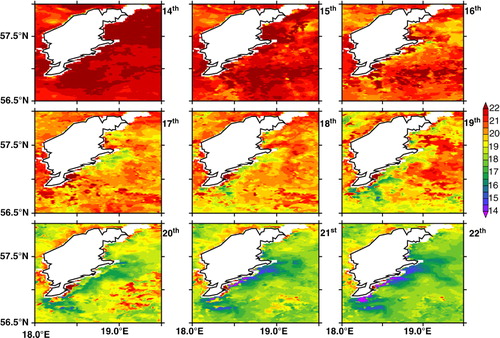
Fig. 4 Daily spatial standard deviation of sea-surface temperature (SST) (°C) in the area surrounding Gotland during 14–22 July 2005 (Period 1).

Period 4 is a shorter period of upwelling with mainly south to south-westerly winds (Fig. 5a). From Fig. 5b–d, it can be seen that the onset of upwelling starts with strong southerly winds. Similar to Period 1, Period 4 shows that during upwelling the atmospheric stratification becomes more stable which is due to the cooling of the sea surface (Fig. 5c). SST drops about four degrees to 6°C and the pCO_2w increases coherent with the SST from 427 µatm at the beginning of the period, and is highest on 26 October with a value of 976 µatm. Period 3 (5–14 October 2008) is a period within the same month as Period 4 with similar properties, although Period 3 includes some occasions with westerly and northwesterly winds. The wind speed during Period 3 is also generally lower, except at the beginning of the period. This results in a somewhat less pronounced effect of upwelling in Period 3 than Period 4.

Fig. 5 Measurements at the Östergarnsholm site during part of Period 4: (a) wind direction (°); (b) wind speed (m s⁻¹); (c) air temperature at two levels (black solid line represents 10 m height and black dashed line at 26 m height), and water temperature from the SAMI sensor (grey solid line) (°C); (c) pCO₂ in air (black solid line) and in water from the SAMI sensor (grey solid line) (µatm).

During Period 4, fluxes of CO₂ at the Östergarnsholm site are measured both at 10 and 26 m height, and both levels of atmospheric measurements are therefore presented in Fig. 5a–c. The wind direction between the two levels does not differ significantly, while the wind speed at the higher level is 0.5–2 m s⁻¹ greater than at the lower level, as expected. The air temperature difference between the two levels is maximum 1.2°C.

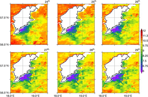
Satellite images of SST during the beginning of Period 4 are shown in Fig. 6. During these days, there is an upwelling area off the southeast coast of Gotland with SST values of less than 8°C (seen as dark green, blue and purple colours in Fig. 6), while the SST off the west coast of Gotland, not affected by upwelling, is 10–11°C. It is noticeable that the area with the coldest temperatures is located south of the in situ measurement station. Although the area of the coldest surface water has approximately the same size as all of the days shown in Fig. 6, it is noticeable that the surroundings are getting more affected by the upwelling as the SST in the whole Gotland region is decreasing.

Fig. 6 As Fig. 3, but during the time period 24–29 October 2008 (Period 4).

4.2. The transfer velocity and fluxes of CO₂

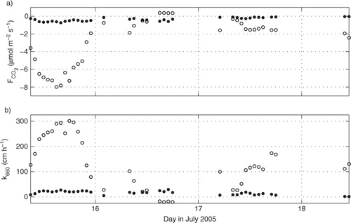
Measurements at the Östergarnsholm site during Periods 1 and 4 are used to describe the air–sea exchange during upwelling in the Gotland region. During the first part of Period 1 when there are atmospheric measurements available, pCO_2w never exceeds the pCO_2a (Fig. 2), and thus the CO₂ flux should be directed downward. Moreover, the flux should decrease as the ΔpCO₂ decreases when pCO_2w increases. Assuming a relatively constant atmospheric pCO₂ of 400 µatm, the direction of the flux is expected to change direction from downward to upward during 23–25 July when the highest pCO_2w values are measured. Unfortunately, measured fluxes are not available during those days.

The measured fluxes (open circles) during Period 1 are shown in Fig. 7a together with fluxes calculated using the bulk formulation [eq. (1)] and the transfer velocity from eq. (2) (filled circles). The bulk flux has a significantly smaller magnitude than the eddy-covariance measured flux, especially during 15 July. A possible explanation could be that the SAMI sensor is not representative for the footprint area of the tower measurements. For south to south-westerly winds, the location of the SAMI should be further to the west if the measurements of SST and pCO_2w are to be representative of the footprint area. Positioning of the SAMI is especially important during periods with horizontal heterogeneity, such as during coastal upwelling. The transfer velocity derived from the measurements is shown together with the calculated transfer velocity [eq. (2)] in Fig. 7b. The measured transfer velocity is significantly larger than the calculated velocity during most of the period. Another possible explanation for the discrepancy between the eddy-covariance and bulk estimated fluxes is that eddy-covariance fluxes are generally higher than mass-balance estimated fluxes, as used for the development of the parameterization by Nightingale et al. (2000), especially during high wind speeds (Garbe et al., 2014).

Fig. 7 (a) Fluxes of CO₂ (µmol m⁻² s⁻¹) and (b) air–sea transfer velocity (cm h⁻¹) during Period 1. Open circles represent in (a) fluxes estimated using the eddy-covariance method, (b) the transfer velocity calculated using eq. (1) and the measured fluxes. Filled circles represent in (a) calculated fluxes using eq. (1) and eq. (2) for the transfer velocity, (b) the transfer velocity according to eq. (2).

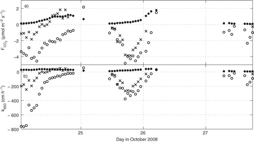
During Period 4, the measured pCO_2w is larger than pCO_2a during the entire period, and the fluxes should therefore be directed upward (Fig. 5d). The ΔpCO₂ increases during this upwelling event, which should result in increasing magnitude of the fluxes. However, as shown in Fig. 8, the measured fluxes (at 10 m height) are mainly negative, that is, downward (open circles). They also have opposite signs to the bulk fluxes (filled circles), which indicates that the SAMI sensor is not representative of the footprint area. Unfortunately, significant parts of the data during Period 4 are lost in the quality control. During this period, fluxes are measured at two levels (at 10 and 26 m). For both heights, the vast majority of the measured fluxes are purely marine influenced, as the wind direction is mainly <210 (see Fig. 5). It can be seen in Fig. 8, that the difference between measured and calculated flux is significantly smaller for the measurements at 26 m height (crosses) than for the lower level. In addition, the flux measured at 26 m more often has the same direction as the calculated flux. This is probably due to the fact that measurements on the higher level have a larger footprint area, which can include a larger horizontal variability than the smaller footprint area associated with the 10 m level measurements. This means that phenomena, such as upwelling, originating from the coast and affecting the CO₂ flux are captured in the measurements at the higher level before, if at all, it is captured at the lower level. The transfer velocity calculated from the measured flux is negative during most of the period, indicating an unphysical counter gradient flux.

Fig. 8 (a) Fluxes of CO₂ (µmol m⁻² s⁻¹) and (b) air–sea transfer velocity (cm h⁻¹) during Period 4. Open circles represent in (a) fluxes at 10 m estimated using the eddy-covariance method, (b) the transfer velocity calculated using eq. (1) and the measured fluxes at 10 m. Crosses represent in (a) fluxes at 26 m estimated using the eddy-covariance method, (b) the transfer velocity calculated using eq. (1) and the measured fluxes at 26 m. Filled circles represent in (a) calculated fluxes using eq. (1) and eq. (2) for the transfer velocity, (b) the transfer velocity according to eq. (2).

4.3. The relation between SST and pCO_2w

The observations at the Östergarnsholm site indicate that there is a strong correlation between SST and pCO_2w during upwelling. Figure 9 shows an example of the relation between pCO_2w and SST during Period 1 (dots), and during 2 d before the upwelling starts (crosses). The correlation coefficient between SST and pCO_2w for the upwelling event during Period 1 is −0.94, while for the 2 d prior to the upwelling period, the correlation coefficient is lower, −0.64. Hence, during upwelling, pCO_2w is strongly linked to SST. This relation is different for the different cases presented here, as illustrated in Fig. 10. The correlation coefficients between SST and pCO_2w are very high also for Periods 2–4, between −0.91 and −0.99 for the four upwelling events (Table 1). We will use this finding, as a first approximation, to utilize satellite-derived SST maps as a proxy for pCO_2w during upwelling (cf. Section 4.4).

Fig. 9 The relation between pCO_2w (µatm) and sea-surface temperature (SST) (°C) (hourly average values) during Period 1 (dots). The crosses represent measurements during 2 d before the upwelling started.

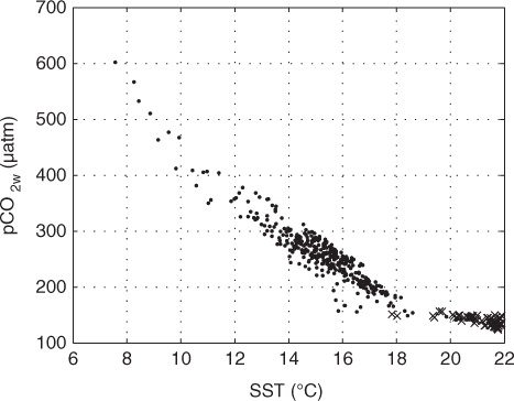
Fig. 10 The relation between pCO_2w (µatm) and sea-surface temperature (SST) (°C) (hourly average values) measured by the SAMI sensor. Black dots represent Period 1, grey dots Period 2, grey circles Period 3 and black circles represent Period 4. The lines represent the fitted linear relation between SST and pCO_2w.

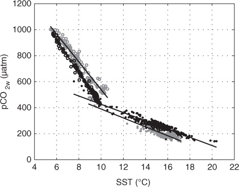
Table 1. Coefficients a and b in the linear relation between SST and pCO_2w, pCO_2w=a+b·SST, during the four upwelling periods

Period	a	B	r
1	−32	747	−0.94
2	−34	732	−0.91
3	−107	1604	−0.97
4	−125	1674	−0.99

Also presented is the correlation coefficient, r, between SST and pCO_2w.

We acknowledge that pCO_2w is affected by biological, chemical and physical processes, for example, phytoplankton influences the dissolved CO₂ through photosynthesis and respiration. In theory upwelling results in an increase of nutrients to the sea surface, which could strongly influence the biological processes leading to a decrease of pCO₂w, which is also observed in some upwelling regions in the World Oceans (see e.g. Borges et al. 2005). However, in the Baltic Sea previous studies have found that the primary production generally decreases during upwelling due to the effects of turbidity, wind speed and decreasing SST (Vahtera et al., 2005; Zalewski et al., 2005). This finding is well in line with ours where we find a strong increase in pCO_2w during upwelling closely correlated with SST.

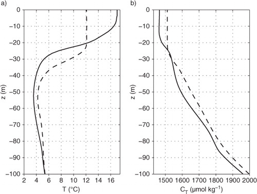
It is noticeable that there is a difference in regime between the July periods (Periods 1 and 2) and the October periods (Periods 3 and 4). The difference in SST–pCO_2w relation between different periods is likely explained by seasonal differences in water column properties. During summer in the Baltic Sea, there is a well-pronounced thermocline which separates the warmer surface water from the colder water below. In the cold and windy winter season, the water column is generally well mixed. Figure 11 shows profiles of temperature and C_T (total inorganic carbon) as an average during 2001–2009 for May and October in the Eastern Gotland basin, calculated using a process-oriented biogeochemical Baltic Sea model (described by e.g. Omstedt et al., 2009). The profile of the temperature illustrates that the thermocline is more pronounced in July than in October, that is, the temperature decreases more rapidly from the sea surface to 100 m in July (Fig. 11a). Hence, during upwelling, SST would probably decrease more in July than in October. C_T, which partly consists of CO₂, is increasing with depth in both July and October (Fig. 11b). The thermocline is found at a deeper level in October than in July; hence, in October CO_2w is detected when the water originates from a greater depth than in July. If water is lifted from greater depths, it would contain more CO₂ compared to if the water has its origin in more shallow water. The influence of properties of the water column described above is shown in Fig. 10; SST decreases more during the July periods compared to the October periods, while pCO_2w increases more during the October periods.

Fig. 11 Water profiles of: (a) temperature (°C); (b) C_T (µmol kg⁻¹) for the Eastern Gotland basin estimated with a one-dimensional biogeochemical Baltic Sea model (Omstedt et al., 2009). The solid line refers to an average of July months during the years 2000–2009, and the dashed line refers to an average of October months during the same period.

4.4. Satellite-derived uptake/release of CO₂

The uptake/release of CO₂ is calculated for the upwelling area on the east coast of Gotland using satellite data during the four upwelling periods. The pCO_2w is calculated using the linear SST–pCO_2w relation shown in Table 1. The CO₂ flux is calculated applying the bulk formulation [eq. (1)], and using the transfer velocity from eq. (2). Atmospheric pCO₂ is estimated using a formula developed by Rutgerssonet al. (2009), where the pCO_2a is expressed as the sum of the global trend, the regional anthropogenic component and the natural seasonal cycle. The actual size of the upwelling area is determined using the upwelling criteria and the satellite data (see Section 2.2.1). The size of the area varies throughout the upwelling periods, although it is generally in the order of 10³ km².

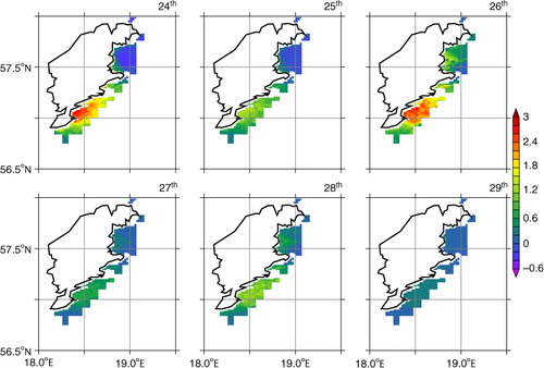
Figure 12 shows calculated CO₂ fluxes based on satellite data of SST during 19–24 July 2005 (Period 1). The area fulfilling the upwelling criteria are coloured and the colours represent the flux (µmol m⁻² s⁻¹). It can be noticed that during this time period, the size of the area is increasing, whereas the magnitude of the fluxes vary. The flux increases in magnitude from 17 to 20 July, and from the 21 July the flux starts to decrease (Fig. 12) due to a change in wind direction to more easterly winds (Fig. 2a). Also, the wind speed strongly affects the magnitude of the calculated flux. Figure 13 shows the same results as Fig. 12 but for 24–27 October 2008 (Period 4). During these days, the fluxes are strong and directed upward, and similar to Period 1, the magnitudes of the flux vary. In addition, along the northeast coast during 24–25 October, there is a small area of weak downward fluxes.

Fig. 12 The coloured area shows estimated fluxes (µmol m² s⁻¹) where upwelling is detected during Period 1 (19–24 July 2005) using the algorithm described in Section 2.2.1. The fluxes are estimated using the satellite sea-surface temperature (SST) and the SST–pCO_2w relation in Table 1, magnitude indicated by the colour bar.

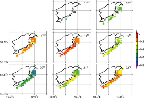
Fig. 13 As Fig. 12, but during the time period 24–27 October 2008. Notice the difference in scale from Fig. 12.

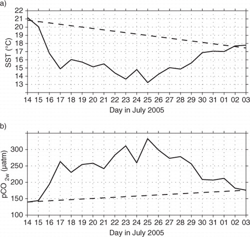
To study the effect of upwelling, the uptake/release of CO₂ for the east coast of Gotland is calculated with and without upwelling. To calculate the uptake/release of CO₂ without upwelling, the SST and the pCO_2w are linearly interpolated between the time before and after the upwelling event, as illustrated for Period 1 in Fig. 14. Furthermore, it is assumed that SST and pCO_2w are homogenous in the Gotland region during the non-upwelling cases. To simplify the estimations, the wind speed is assumed to be homogenous in the region during the upwelling cases as well as the non-upwelling cases.

Fig. 14 Daily averaged sea-surface temperature (SST) (°C) and pCO_2w (µatm) during 14 July–3 August 2005 (Period 1). The solid lines are measured values showing upwelling with decreasing SST and increasing pCO_2w. The dashed lines illustrate interpolated values assuming no upwelling occurred during this period.

The results from the budget calculations are shown in Table 2. For Periods 1 and 2, the July periods, the CO₂ uptake decreases during upwelling by 5.0 and 5.4 Gg, respectively. This corresponds to a relative decrease of 1 and 59%. During Periods 3 and 4, the October periods, the CO₂ release increases by 15.4 and 23.4 Gg, respectively. The corresponding relative increases are 211 and 250%. Hence, upwelling makes the area off the east coast of Gotland less of a sink of CO₂.

Table 2. The uptake/release of CO₂ (Gg) calculated without (A) and with (B) upwelling during the four upwelling events in the upwelling area off the south east coast of Gotland

Period	A	B	AD	ARD
1	−25.5	−20.5	5.0	19
2	−9.2	−3.8	5.4	59
3	+7.3	+22.7	15.4	211
4	+9.4	+32.8	23.4	250

Also presented are the absolute difference (AD) (Gg), and the absolute relative difference (ARD) (%), of the uptake/release with and without upwelling.

5. Discussion

The impact of upwelling on the total carbon budget of the entire Baltic Sea may be significant, as indicated by the following rough estimate. Assuming the total coastline in the Baltic Sea affected by upwelling is 2800 km, and that the effect extends 20 km offshore (Gidhagen, 1987), the area affected by upwelling would thus be 56 000 km². During May to September, this area is affected by upwelling 25–30% of the time (Gidhagen, 1987; Lehmann et al., 2012). No similar estimation exists for the period October–April. In this calculation, we make a conservative assumption that upwelling is present 10% of the time during this period. An upwelling event lasts from a few days up to 1 month. Thus, assuming that an upwelling event lasts 14 d is reasonable. This would mean that the coastal area in the Baltic Sea is affected by approximately four upwelling events per year. One upwelling event in an area of 1000 km² can cause a decrease in the CO₂ uptake by 5 Gg (Table 2). This would mean that, due to upwelling, the CO₂ uptake in the Baltic Sea might decrease by 1120 Gg yr⁻¹ assuming that the strength of the upwelling events are of similar magnitudes in all basins of the Baltic Sea. The decrease in CO₂ uptake can be compared to the calculated net uptake of 3998 Gg C yr⁻¹ by Norman et al. (2013), and the estimated source of 4543 Gg C yr⁻¹ by Kulinski and Pempkowiak (2012). Thus, including upwelling in the estimates has the potential to change the Baltic Sea uptake by 25%. This is of course a ‘back-of-the-envelope’ calculation with significant uncertainties. However, it gives us an idea as to what extent the Baltic Sea CO₂ budget can be affected by upwelling.

6. Summary and conclusions

Four upwelling events off the east coast of Gotland are selected and analyzed. Two of the periods are July periods (Period 1 and 2), and two of the periods are October periods (Period 3 and 4). The measured fluxes and transfer velocities do not agree well with the corresponding values calculated from bulk formulae, measured values being much larger. This is probably partly due to the difficulties with representativeness of the transfer velocity calculated from measurements during upwelling at this site. The pCO_2w measurements appear not to be representative for the footprint area of the flux when the wind direction is south to southwest during upwelling yielding erroneous estimates of k. The measurements from 26 m height showed somewhat better agreement with the bulk estimates. For these data, the footprint area is larger compared to the lower level flux measurements and thus it is more likely that the heterogeneity in the sea surface due to the upwelling is captured. Additionally, there is a difference based on the method of measured and bulk estimated fluxes used in this study, which yield higher fluxes during high wind speeds for the measured compared to the bulk estimated fluxes.

There is a strong correlation between in situ measured SST and pCO_2w during the selected upwelling events, and satellite SST data are therefore used to estimate pCO_2w over a larger region. The October and July periods appear to be of different regimes with respect to pCO_2w–SST correlation. This difference is most likely due to a combination of seasonal differences in variables such as thermal stratification, and C_T in the water column. As the relation between SST and pCO_2w is somewhat different for different upwelling events, we have not developed a generally valid relation. However, there is a seasonal variability in the SST–pCO_2w relation. If more upwelling periods during different seasons were analyzed, it might be possible to construct an upwelling relation for the pCO_2w which would be a function of the time of year, or a function due to various physical or biological forcing.

Furthermore, the wind-dependent expression for the transfer velocity [eq. (2)] may not be optimal during upwelling. As shown by Rutgersson and Smedman (2010) and Rutgersson et al. (2011), standard bulk formulae for flux calculations are not valid during conditions with a stably stratified atmosphere and large mixing in the water. Such conditions are valid also during upwelling. However, this can be remedied. Similarly to what was done in Rutgersson et al. (2011), upwelling effects on k could be included in the physically based parameterization NOAA-COARE algorithm (Fairall et al., 2000; Jeffery et al., 2007). However, a more accurate description of the behaviour of k during upwelling is needed to implement the effects into the algorithm.

The effect of upwelling on the air–sea CO₂ fluxes is evident for the upwelling area with a change of the uptake/release of 19–250%. During the July periods, the uptake of CO₂ is decreased, while during the October periods the release of CO₂ is increased. Since coastal upwelling frequently occurs in the Baltic Sea, upwelling is expected to have a major impact on the total Baltic Sea carbon budget. Norman et al. (2013) used a Baltic Sea model, and showed that the Baltic Sea is a net sink of atmospheric CO₂. This model did not capture upwelling, thus, if upwelling was included, it would probably make the Baltic Sea a smaller sink or even a net source.

Acknowledgements

Gisela Tschersich at German Federal Maritime and Hydrographic Agency, Hamburg (BSH) is gratefully acknowledged for providing the satellite data for SST. The Swedish meteorological and hydrological institute (SMHI) is acknowledged for providing wind data from the SMHI measurement site at Östergarnsholm. The authors thank Kimmo Kahma and Heidi Pettersson at the Finnish Meteorological Institute for sea-surface temperature data and assistance with the SAMI sensor. Heidi Pettersson is also acknowledged for valuable comments on the article. The authors thank Anders Omstedt at the University of Gothenburg for access to the Baltic Sea model. Furthermore, William Drennan at University of Miami, Rosenstiel School of Marine and Atmospheric Sciences is acknowledged for useful comments on the article. Gaëlle Parad is gratefully acknowledged for discussions on upwelling and comments on the results. The authors also thank David Sproson for proofreading the article. Additionally, the authors thank the two anonymous reviewers who helped improve the article.