Comment on Qian et al. 2008: La Niña and El Niño composites of atmospheric CO₂ change

Abstract

It is well known that interannual extremes in the rate of change of atmospheric CO₂ are strongly influenced by the occurrence of El Niño-Southern Oscillation (ENSO) events. Qian et al. presented ENSO composites of atmospheric CO₂ changes. We show that their composites do not reflect the atmospheric changes that are most relevant to understanding the role of ENSO on atmospheric CO₂ variability. We present here composites of atmospheric CO₂ change that differ markedly from those of Qian et al., and reveal previously unreported asymmetries between the effects on the global carbon system of El Niño and La Niña events. The calendar-year timing differs; La Niña changes in atmospheric CO₂ typically occur primarily over September–May, while El Niño changes occur primarily over December–August. And the net concentration change is quite different; La Niña changes are about half the size of El Niño changes. These results illustrate new aspects of the ENSO/global carbon budget interaction and provide useful global-scale benchmarks for the evaluation of Earth System Model studies of the carbon system.

• carbon dioxide
• El Nino
• La Nina
• atmospheric variability
• emissions
• concentration change

1. Introduction

It has been known since the 1970s that interannual changes in CO₂ concentration are strongly correlated with El Niño-Southern Oscillation (ENSO) (e.g. Bacastow, 1976; Elliot et al., 1991). Recent efforts to explain the processes that link ENSO and atmospheric CO₂ variability have focused on the effects that ENSO impacts on seasonal weather conditions might have on the net terrestrial ecosystem exchange of CO₂; the ENSO influence on the oceanic exchange is currently thought to be smaller than, and out of phase with, the net CO₂ fluxes needed to explain the link (Feely et al., 1999; Bousquet et al., 2000; Le Quéré et al., 2003; Peylin et al., 2005; Park et al., 2006).

Climate-driven terrestrial biosphere models have been able to reproduce many aspects of the estimated terrestrial fluxes, including the broad-scale correlation between atmospheric CO₂ and ENSO behaviour (Kindermann et al., 1996; Tian et al., 1998; Gerard et al., 1999; Jones et al., 2001; Hashimoto et al., 2004; Ichii et al., 2005; Zeng et al., 2005; Qian et al., 2008). Different modelling studies, however, have reached different conclusions about the identities of the dominant ecosystem processes (e.g. photosynthesis, respiration, fires) and climate forcings (e.g. temperature, precipitation, solar variability). Stricter observational constraints are needed to help evaluate model performance. In particular, clarity is needed in as much detail as possible about the CO₂ changes that have taken place during each El Niño and La Niña event, as well as in the event-average.

Composite analysis has been used previously to identify the disruptions of atmospheric and oceanic circulation in the tropical Pacific (e.g. Rasmussen and Carpenter, 1982; Larkin and Harrison, 2002) and global seasonal weather anomalies (e.g. Ropelewski and Halpert, 1987, 1989; Larkin and Harrison, 2005; Chiodi and Harrison, 2013) that are common to El Niño and La Niña events. Composite analysis has recently been extended to El Niño and La Niña effects on the rate of change of atmospheric CO₂ concentration by Qian et al. (2008) (Q08 hereafter), who use ENSO composites of the CO₂ growth rate to help evaluate the performance of their terrestrial biosphere model.

Based on methodology that is criticised herein, Q08 found that the differences between the carbon cycle impacts from one El Niño event to the next ‘can be larger than the difference between typical El Niño and La Niña events’ (notwithstanding the unusual events of 1991–93) and thus mainly treated La Niña events as ‘negative El Niño events’ when evaluating their model. When differences between La Niña and El Niño effects were discussed by Q08, they claimed that the initial impact of La Niña on atmospheric CO₂ growth begins a couple of months later than in El Niño and persists much longer than in the El Niño case (well into ENSO Year 2; e.g. 1999 in the case of the large 1997–98 El Niño event).

Recently, Guerney et al. (2012) (G12 hereafter) have examined the correlation of ENSO and regional estimates of net carbon exchange and concluded that the ENSO warm-phase explains >70% of the variability in tropical net carbon exchange. But no evidence for this El Niño-dominance was uncovered by the Q08 examination of the atmospheric CO₂ record. It is difficult to see how the Q08 characterisation of El Niño and La Niña effects on atmospheric CO₂ changes and the G12 results can both be qualitatively correct.

We have constructed seasonal-average and annual-average composites of atmospheric CO₂ changes over the Mauna Loa time series using well-accepted identifiers of El Niño and La Niña years. These composites differ greatly from those reported by Q08. After some exploration, we were able to reproduce the composites of atmospheric CO₂ variability considered by Q08 and so understand the source of these differences. Q08 did not composite the CO₂ changes averaged over particular periods; rather their approach yields averages of the difference between two monthly average CO₂ values spaced 12 months apart. The averages we report are those which are relevant to understanding the relationships between El Niño and La Niña and the global carbon cycle.

Our results reveal that La Niña changes involve about half as much CO₂ and begin sooner in the calendar-year than in the El Niño case, but the changes persist for a similar number of seasons in each case; La Niña changes typically occur primarily over September of ENSO Year 0 to May of ENSO Year 1, while El Niño changes occur over December of ENSO Year 0 to August of ENSO Year 1. Thus, our results disagree in many respects with the Q08 results and confirm the central G12 finding that El Niño affects the carbon cycle more strongly than La Niña. Furthermore, we show that the La Niña changes, though statistically significant in their own right, are not nearly as robust (i.e. have the same sign and similar amplitude from event to event) as the El Niño effects; over the time for which the Mauna Loa record is available, each of the (11) years in the top 20% in terms of anomalous (notwithstanding the anthropogenic rise) concentration growth has El Niño status based on the commonly used definitions. This is not nearly true in the opposite sense for the La Niña case.

2. Data and methods

Monthly average CO₂ concentration values measured at the Mauna Loa, HI, USA site are provided by the Scripps Institute (Keeling et al., 2001, 2012), and available, dating back to 1958, from the website http://scrippsCO2.ucsd.edu/data/in_situ_CO2/monthly_mlo.csv. We base our analysis on seasonal and annual averages using all years and seasons without missing values (1958 and 1964 are excluded due to data gaps).

Annual changes in CO₂ concentration are determined by first forming 12-month averages that span March of one year to February of the next and then differencing adjacent 12-month averages. The mean annual cycle is thereby removed by differencing 12-month periods in the annual case. Other start/end months were preliminarily considered. The March to February Year +1 case yielded the maximum composite anomalies discussed below. The seasonal rate of change of CO₂ concentration is determined from the difference between adjacent seasonal CO₂ concentration values, in this case taken as December through February, ‘DJF’, March through May ‘MAM’, June through August ‘JJA’ and September through November ‘SON’. The respective long-term seasonal mean change (e.g. MAM minus DJF CO₂ change values averaged over all years in record) is then subtracted in this case to remove the average effect of the seasonal cycle over the given pair of seasons.

The trend caused by emissions from fossil fuel burning and cement production is removed from the Mauna Loa record prior to calculating the annual and seasonal concentration changes to highlight the changes that occur over interannual time scales (as done also, e.g. in Elliot et al., 1991). We use the annual estimates of these emissions provided by Boden et al. (2011), available at http://cdiac.ornl.gov/ftp/ndp030/global.1751_2008.ems, to do this. In this case, the (constant) fraction of annual fossil fuel and cement emissions (‘airborne fraction’) that yields a remaining time series with zero mean is removed. Trials showed that our conclusions are robust to reasonable changes in the details of this procedure (e.g. using an airborne fraction with a best-fit linear trend and/or including the available estimates of emissions from land-use change). Hereafter, the changes in CO₂ concentration that remain after the anthropogenic trend and seasonal cycle have been removed will be referred to as the ΔCO₂ anomaly.

When referring to ENSO events, we follow the convention used in the previous ENSO composite studies (e.g. Rasmussen and Carpenter, 1982; Larkin and Harrison, 2002) that identifies the year in which ENSO anomalies typically grow from background levels to maturity as Year 0, and the following as Year 1, etc. ENSO-related disruption of the usual oceanic and atmospheric circulation in the tropical Pacific typically peaks at the end of ENSO Year 0/beginning of ENSO Year 1 (e.g. Larkin and Harrison, 2002).

We use the NIÑO3 index averaged from September through November (ENSO Year 0) as a measure of ENSO state. Larkin and Harrison (2002) showed that many ENSO-related tropical Pacific anomaly conditions peak at this time of year. The NIÑO3 index is the sea-surface temperature (SST) anomaly averaged in the tropical Pacific region bounded by 150°W and 90°W and 5°S and 5°N. For SST information, we use the monthly averaged Hadley Centre SST data set, available at their website: http://www.metoffice.gov.uk/hadobs/hadisst/ (Rayner et al., 2003). In a preliminary correlation analysis, the September-through-November (SON) averaged NINO3 case yielded the highest correlation (0.7) with ΔCO₂ anomaly among the cases considered (we also considered, e.g. NINO3.4, the Southern-Oscillation Index and the ‘MEI’, or multivariate ENSO index, as well as averages over the other 3-month seasons).

3. Composite results

The annually averaged (not yet detrended) rate of change of atmospheric CO₂ (black curve) is shown in Fig. 1, along with recent estimates (Boden et al., 2011) of CO₂ emissions from fossil fuel burning and cement production (green bars). The interannual variability seen in the CO₂-change record is much larger than, and therefore cannot be explained by the interannual variability seen in the estimated emissions. The annual changes in CO₂ concentration that remain after the trend from the fossil fuel and cement emissions is removed are plotted in Fig. 2. The range of the year-to-year changes plotted in Fig. 2 is comparable to the average annual atmospheric CO₂ growth rate and on the same order of magnitude of the absolute emissions themselves (Fig. 1). Thus, in any given year, the net atmospheric CO₂ change may be strongly influenced by the natural variability of the global carbon cycle, and not just emissions. The strong El Niño years, identified here as the years with SON averages of the NIÑO3 SSTA index >1 time series standard deviation (σ), are shown by the red circles in Fig. 2 (1965–66, 1972–73, 1976–77, 1982–83, 1987–88 and 1997–98). It is clear that many of the years with the largest anomalous CO₂ increases are El Niño years.

Fig. 1 The annual change in atmospheric CO₂ concentration measured at the Mauna Loa site (black curve) and estimates of the annual CO₂ emissions from fossil fuel burning and cement production (green bars). As is usefully done elsewhere (Prentice et al., 2001), the ratio of the two Y-axes is chosen such that the rate of CO₂ change would track the emissions curve if all emissions were accounted for and remained in the atmosphere; the interannual variability seen in the CO₂-change record is much larger than, and therefore cannot be explained by the interannual variability seen in the estimated emissions.

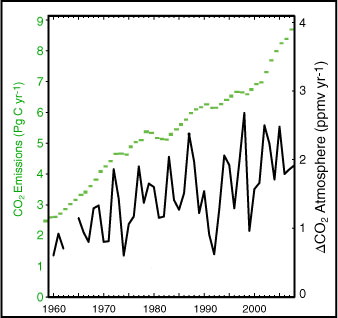
Fig. 2 Annual changes in CO₂ concentration (left-hand Y-axis) after removing the trend from emissions. Estimated net carbon equivalent given by the Y-axis on the right. Filled red circles mark years with SON NIÑO3 > 1σ; blue triangles for years with SON NIÑO3 <1σ.

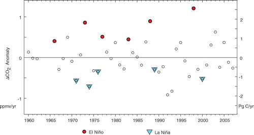
The difference between the average ΔCO₂ anomaly during these El Niño events and all other years in record is +0.83 ppmv yr⁻¹, which is highly statistically significant (exceeds the 99.99% confidence level based on the classic Student's t difference-of-two-means test) and equivalent to an atmospheric gain of roughly +1.8 Pg C yr⁻¹, which is about two-thirds of the average annual growth rate seen over the last 50 yr.

The strong La Niña years (SON NIÑO3<−1σ) are highlighted by blue triangles in Fig. 2 (1970–71, 1973–74, 1975–76, 1988–89 and 1999–2000). It can be seen that many of the largest anomalous decreases, which in absolute terms are the years in which CO₂ rose less than expected based on just anthropogenic emissions, are La Niña years. The amplitude of the apparent La Niña effect, however, is not as large as in the El Niño case; the difference between the average ΔCO₂ anomaly during the identified La Niña events and all other years in record is −0.54 ppmv yr⁻¹, which, although smaller in amplitude than the El Niño effect, remains statistically significant at the 99% level and is equivalent to an atmospheric loss of roughly −1.1 Pg C yr⁻¹.

The El Niño events of 1982–83 and 1997–98 experienced the largest warm central Pacific SSTAs in the recent decades. It is notable that even if these two large-SSTA events are omitted, the average El Niño effect on CO₂ concentration (+0.77 ppmv yr⁻¹ in this case) remains substantially larger than its aforementioned La Niña counterpart (−0.54 ppmv yr⁻¹). This amplitude asymmetry, therefore, cannot be explained solely by the inclusion of these two unusually large (based on tropical Pacific anomaly state) events in the El Niño case.

Inspection reveals that in addition to amplitude, there is a substantial difference in the robustness, or event-to-event consistency, of the atmospheric CO₂ responses to La Niña and El Niño. This can be seen more easily in Fig. 3, where the ΔCO₂ anomaly values from all the years considered with a complete CO₂ record are shown in rank-order. El Niño years consistently rank highest; six of the eight top years are among the identified strong El Niño years. However, the identified strong La Niña years do not comparably dominate among the group of years with the largest negative ΔCO₂ anomalies. Apparently, conditions other than those that occur during La Niña events occur fairly frequently and also produce comparable negative CO₂ concentration change anomalies.

Fig. 3 Rank-order ΔCO₂ anomalies with strong La Niña and El Niño years, based on SON values of the NIÑO3 index, shaded blue and red, respectively. Other years with ENSO-status based on the current NOAA Historical El Niño definition are shown with speckled shading.

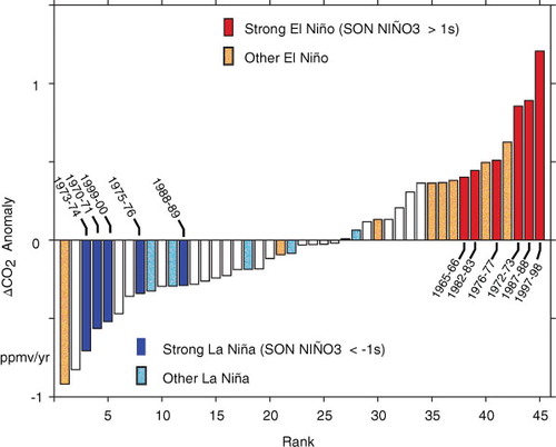
Further examination shows that substantial anomalous increases in CO₂ concentration are seen among many other years that have some type of El Niño status based on the commonly used definitions but do not make our ‘strong’ list. The composite average ΔCO₂ difference of these secondary El Niño events, identified here as years that have ENSO status based on the current National Oceanic and Atmospheric Administration (NOAA) definition, but are not among the identified strong events (see speckled orange shading in Fig. 3), has a value of 0.31 ppmv yr⁻¹ if the unusual 1991–92 event is excluded and remains moderately statistically significant (p=0.92) at this magnitude. Including 1991–92, however, would substantially lower this value. Each of the 11 top-ranked years has El Niño-status based on the current NOAA Historical El Niño definition. The secondary La Niña events (speckled light-blue shading in Fig. 3) do not have a statistically significant effect on CO₂ concentration. The El Niño effect on atmospheric CO₂ is far more robust than is the La Niña effect.

We note that the Q08 lists of El Niño and La Niña years are different than ours, but we have found that the basic result that El Niño CO₂ changes are typically much larger in amplitude than La Niña changes is recovered using their lists of years and our measure of annual CO₂ change. Q08 considered a period that is about half as long as is considered here (Q08 used 1980–2004, except the 1991–93 period following the eruption of Mount Pinatubo) and used a lower threshold (∣MEI∣ >0.75σ) to identify four La Niña and four El Niño years in that period. Thus, their lists include a mix of what are classified here as strong and secondary ENSO years (Q08 warm-ENSO: 1982–83, 1986–87, 1994–95, 1997–98; Q08 cool-ENSO: 1984–85, 1988–89, 1995–96, 1998–99; strong in bold-type). Based on our findings that secondary El Niño years have statistically significant effects but secondary La Niña years do not, it should be expected that the Q08 lists, which identify mainly secondary years in the La Niña case, yield a much stronger CO₂ change in the El Niño than La Niña case. Indeed, this is what occurs when annual ΔCO₂ anomalies are composited based on the Q08 lists; the Q08-list El Niño composite change is +0.63 ppm yr⁻¹ (relative to all other years in record) which is statistically significant (p>0.99), and more than three times the Q08-list La Nina change (−0.18 ppm yr⁻¹), which is not statistically significant at standard confidence intervals. Thus, the differences between our and Q08's composites cannot be explained by the use of different ENSO-year lists in the compositing methods.

Conspicuously, the largest negative ΔCO₂ anomaly in the study period occurs in the El Nino year of 1991–92, showing that, as strong as the El Niño effect on atmospheric CO₂ is, it can be overcome by other processes. Although different effects of the volcanic aerosols from the 1991 Mount Pinatubo eruption have been hypothesised to explain this large negative ΔCO₂ anomaly (Farquhar and Roderick, 2003; Gu et al., 2003) the reasons for it remain largely unknown (Peylin et al., 2005).

In the review process, the issue of the possible effects of volcanic aerosols in other years on our ΔCO₂ composites was brought up. Examination of the published estimates of volcanic aerosol optical depth (e.g. Ammann et al., 2003) suggests that in addition to 1991–92, the El Niño events of 1965–66 and 1982–83, along with the La Niña of 1975–76 occurred during times in which the volcanic aerosol optical depth was not small (e.g. not less than 10% of the peak value seen in the study period; cf. Guerney et al., 2012). With these other years removed, the ΔCO₂ anomaly composite increases somewhat from +0.83 ppmv yr⁻¹ to +0.95 ppmv yr⁻¹ in the El Niño case, and varies only slightly (−0.54 ppmv yr⁻¹ and −0.57 ppmv yr⁻¹, respectively) in the La Niña case. Thus, the asymmetry between the amplitudes of these composites is not caused by the effects of volcanic aerosols.

Further examination of the full Mauna Loa record reveals that other differences in the carbon system behaviour between La Niña and El Niño events are apparent at time scales shorter than annual averages. Examination of the seasonal ΔCO₂ anomalies during the five strong La Niña and six strong El Niño years reveals that not all seasons are equally important for understanding the variations between ΔCO₂ and ENSO variability (see Table 1). The La Niña composites show statistically significant ΔCO₂ anomalies over both the DJF-minus-SON and MAM-minus-DJF seasonal changes, but not any of the others (all cases from ENSO Year 0 to 2 were examined, but only those listed in Table 1 reached statistical significance at standard confidence intervals). In the El Niño case, significant effects are also seen across two pairs of seasonal changes, but they begin later in the calendar-year with the MAM-minus-DJF composite and extend to the following JJA-minus-MAM composite. The results at annual and seasonal time scales are consistent in the sense that the El Niño effect is larger than the La Niña effect in each case and changes in concentration from boreal winter-to-spring (MAM-minus-DJF) are key. Fig. 4 summarises the average differences in amplitude and timing between the effects of the strong La Niña and strong El Niño events’ composites on changes in atmospheric CO₂.

Fig. 4 Summary of strong La Niña and El Niño effects on interannual atmospheric CO₂ concentration variability. The season-to-season CO₂ changes illustrated here are those that yield statistically significant composite ΔCO₂ anomalies (all season-to-season changes from ENSO Year 0 to 2 were evaluated for their statistical significance).

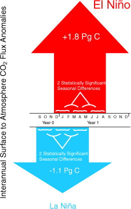
Table 1. Composite seasonal changes in atmospheric CO₂ concentration at the Mauna Loa site for the 5 strong La Niña and 6 strong El Niño events (ENSO Year 0 to Year +1)

Seasons considered	La Niña ΔCO2 composite	El Niño ΔCO2 composite
DJF minus SON (Year 1/0)	−0.29*	Not significant
MAM minus DJF (Year 1)	−0.25	0.34
JJA minus MAM (Year 1)	Not significant	0.42

Values are in ppmv yr⁻¹. Bold type shows values significant at the 95% level. All other values shown are significant at the 90% level, or better, except for the value noted by the asterisk, for which p=0.89. All seasonal pairs from ENSO Year 0 to 2 were considered. Only those shown yield statistically significant results.

We also looked at monthly time scale behaviour, but found there is too much variability to yield statistically useful results. Seasonal time resolution seems to be the shortest on which reliable statistics are found.

4. Discussion and conclusions

The composite net atmospheric CO₂ change results presented here tell a clear story about the differences in changes associated with El Niño and La Niña periods. The El Niño period composites are typical of changes for individual El Niño events (excepting 1991–92), while the La Niña events show greater event-to-event variability. El Niño period changes are roughly twice as large as La Niña period changes (and of the opposite sign). Most of the change occurs over three seasons in both El Niño and La Niña years, but El Niño effects begin later in the calendar-year and so continue longer into the following year than do La Niña changes. Furthermore, this substantial asymmetry between the El Niño and La Niña effects on the global carbon budget is not qualitatively dependent on our choice of La Niña and El Niño years; the Q08 list of years yields a similar difference in effect.

G12 have also described an asymmetry in El Niño and La Niña carbon system effects, although in less detail than we present. These results, however, are very different from those of Q08. We show that the Q08 results are so different because Q08 did not average the CO₂ change over the periods they were interested in. To ensure that we are correct in this interpretation, we have found that the Q08 (their Fig. 1) results are obtained by applying a 12-month running mean filter to the month-to-month change in CO₂ observed at the Mauna Loa site. It is important to note that the Q08 computation does not evaluate the 12-month average CO₂ concentration change (as our calculation does). Rather, the Q08 calculation computes the change in CO₂ concentration between the end-points of the running-mean period. As they have applied it, it generates the difference between two monthly average CO₂ values spaced 12 months apart. This approach would not be helpful in the evaluation of sub-annual concentration changes both because it is the period-of-interest net change that is carbon-budget-relevant and because the difference between two monthly averages would be highly susceptible to the large amounts of month-to-month variability seen in the Mauna Loa record, much of which is unrelated to ENSO. If the quantities of interest are the net change in the carbon system during El Niño and La Niña events and the seasons in which this predominantly occurs, the composites presented above are the ones of relevance.

From an earth system perspective, we wish to understand not only the net changes and the timing of the changes in the carbon system, but also the mechanisms that are responsible for the observed behaviour. Given the limited amounts of earth system observations available, earth system models that include carbon system processes will likely be the predominant near-term source of hypotheses about ENSO/carbon system mechanisms. Some remarks can nonetheless be offered. In particular, whereas the available oceanic observations indicate that oceanic changes during ENSO are of the wrong sign and too small to be able to account for the behaviour reported here (e.g. Peylin et al., 2005; Park et al., 2006), changes in the timing and magnitude of the seasonal cycle of terrestrial vegetation clearly deserve attention, and tropical forests are of particular interest because they are estimated to involve large CO₂ exchanges. A specific example is Huete et al. (2006), who show that the Amazon rainforest ‘greens-up’ during the typically dry months of July through November (canopy greenness is usually at its seasonal maximum late in the calendar-year). The atmospheric CO₂-change composites described herein reveal that the seasons following this green-up (and coinciding with it in the La Niña case) are among those that experience the largest ENSO effects on CO₂ concentration. Examining whether the timing and character of the ENSO-related seasonal weather anomalies are able to force ecosystem responses in such regions that reproduce the newly revealed asymmetry and timing of the observed El Niño and La Niña CO₂ changes deserves additional attention.

Even once the composite changes are rationalised, particularly the fact that El Niño events on average involve approximately 50% larger CO₂ concentration changes than La Niña events, with different seasonal timings, there is more to be investigated associated with event-to-event variation. In particular, larger and smaller (using the SSTA measure of strength) El Niño events seem to give comparable CO₂ changes, while smaller La Niña events produce much smaller CO₂ changes than do larger La Niña events.

As with any composite study, although we have used the longest directly measured record of atmospheric CO₂ currently available to compute the composites discussed herein, the number of ENSO events resolved in this (50 yr) record is nonetheless limited. As our planet's climate varies ENSO statistics may change and so may the carbon system behaviour during El Niño and La Niña events. Our results will merit revisiting in the future.

It is well known that the magnitude of interannual variability associated with El Niño and La Niña events is large enough to pose a challenge to efforts to estimate changes in multi-decadal trends in the planetary carbon system (Canadell et al., 2007; Raupach et al., 2008; Le Quéré et al., 2009; Chiodi and Harrison, 2012). ENSO has strong multi-decadal variability and in some periods either El Niño or La Niña events may predominate. Thus, the statistics of ENSO variability must be taken into consideration when trend estimates are made. Our results indicate that attempting to remove ENSO effects for trend analyses by simple regression techniques is not wise. Detecting changes in long-term trends in the carbon system must be done in full awareness of the uncertainties.

5. Acknowledgments

This work was supported by NOAA Pacific Marine Environmental Laboratory Contribution 3509; by NOAA's Climate Observation Program, NOAA's Pacific Marine Environmental Laboratory; and by the Joint Institute for the Study of the Atmosphere and Ocean (JISAO) under NOAA Cooperative Agreement No. NA17RJ1232. This is also JISAO Contribution 1799. The authors thank the two anonymous reviewers for their time and helpful comments.

References

- Ammann C. M. , Meehl G. A. , Washington W. M. , Zender C. S . A monthly and latitudinally varying volcanic forcing dataset in simulations of 20th century climate. Geophys. Res. Lett. 2003; 30(12): 1657. 10.1029/2003GL016875.
- Bacastow R . Modulation of atmospheric carbon dioxide by the Southern oscillation. Nature. 1976; 261: 116–118.
- Boden T. A. , Marland G. , Andres R. J . Global, Regional, and National Fossil-Fuel CO2 Emissions. 2011; Oak Ridge, TN, USA: Carbon Dioxide Information Analysis Center, Oak Ridge National Laboratory, US Department of Energy. 10.3334/CDIAC/00001_V2011.
- Bousquet P. , Peylin P. , Ciais P. , Le Quéré C. , Friedlingstein P. , co-authors . Regional changes in carbon dioxide fluxes of land and oceans since 1980. Science. 2000; 290(5495): 1342–1346.
- Canadell J. G. , Le Quéré C. , Raupach M. R. , Field C. B. , Buitenhuis E. , co-authors . Contribution to accelerating atmospheric CO2 growth from economic activity, carbon intensity, and efficiency of natural sinks. Proc. Natl. Acad. Sci. U.S.A. 2007; 104: 18866–18870.
- Chiodi A. M. , Harrison D. E . Determining CO2 airborne fraction trends with uncertain land use change emission records. Int. J. Clim. Change. 2012; 3(1): 79–88.
- Chiodi A. M. , Harrison D. E . El Niño impacts on seasonal U.S. atmospheric circulation, temperature, and precipitation anomalies: the OLR-event perspective. J. Clim. 2013; 26: 822–837.
- Elliot W. P. , Angell J. K. , Thoning K. W . Relation of atmospheric CO2 to tropical sea and air temperatures and precipitation. Tellus. B. 1991; 43: 144–155.
- Farquhar G. D. , Roderick M. L . Pinatubo, diffuse light, and the carbon cycle. Science. 2003; 299: 1997–1998.
- Feely R. A. , Wanninkhof R. , Takahashi T. , Tans P . Influence of El Niño on the equatorial Pacific contribution of atmospheric CO2 accumulation. Nature. 1999; 398: 597–601.
- Gerard J. , Nemry B. , Francois L. , Warnant P . The interannual change of atmospheric CO2: contribution of subtropical ecosystems?. Geophys. Res. Lett. 1999; 26: 243–246.
- Gu L. , Baldocchi D. , Wofsy S. C. , Munger J. W. , Michalsky J. , co-authors . Response of a deciduous forest to the Mount Pinatubo eruption: enhanced photosynthesis. Science. 2003; 299: 2035–2038.
- Guerney K. R. , Castillo K. , Li B. , Zhang Z . A positive carbon feedback to ENSO and volcanic aerosols in the tropical terrestrial biosphere. Glob. Biogeochem. Cycles. 2012; 26: GB1029. 10.1029/2011GB004129.
- Hashimoto H. , Nemani R. R. , White M. A. , Jolly W. M. , Piper S. C. , co-authors . El Niño-Southern oscillation induced variability in terrestrial carbon cycling. J. Geophys. Res. 2004; 109: D23110. 10.1029/2004JD004959.
- Huete A. R. , Didan K. , Shimabukuro Y. E. , Ratana P. , Saleska S. R. , co-authors . Amazon rainforests green-up with sunlight in dry season. Geophys. Res. Lett. 2006; 33: L06405. 10.1029/2005GL025583.
- Ichii K. , Hashimoto H. , Nemani R. , White M . Modeling the interannual variability and trends in gross and net primary productivity of tropical forests from 1982 to 1999. Glob. Planet. Change. 2005; 48: 274–286.
- Jones C. D. , Collins M. , Cox P. M. , Spall S . The carbon cycle response to ENSO: a coupled climate-carbon cycle model study. J. Clim. 2001; 14: 4113–4128.
- Keeling C. D. , Piper S. C. , Bacastow R. B. , Wahlen M. , Whorf T. P. , co-authors . Exchanges of Atmospheric CO2 and 13CO2 with the Terrestrial Biosphere and Oceans from 1978 to 2000. I. Global Aspects. SIO Reference Series, No. 01–06. 2001; San Diego: Scripps Institution of Oceanography. 88.
- Keeling R. F. , Piper S. C. , Bollenbacher A. F. , Walker S. J . Atmospheric CO2 Concentrations (ppm) Derived from In Situ Air Measurements at Mauna Loa, Observatory, Hawaii: Latitude 19.5°N Longitude 155.6°W Elevation 3397m. 2012. Scripps Institution of Oceanography CO2 Program. Online at: http://scrippsco2.ucsd.edu .
- Kindermann J. , Wurth G. , Kohlmaier G . Interannual variation of carbon exchange fluxes in terrestrial ecosystems. Glob. Biogeochem. Cycles. 1996; 10: 737–755.
- Larkin N. K. , Harrison D. E . ENSO warm (El Niño) and cold (La Niña) event life cycles: ocean surface anomaly patterns, their symmetries, asymmetries, and implications. J. Clim. 2002; 15(10): 1118–1140.
- Larkin N. K. , Harrison D. E . Global seasonal temperature and precipitation anomalies during El Niño autumn and winter. Geophys. Res. Lett. 2005; 32: L16705. 10.1029/2005GL022860.
- Le Quéré C. , Aumont O. , Bopp L. , Bousquet P. , Ciais P. , co-authors . Two decades of ocean CO2 sink and variability. Tellus. B. 2003; 55: 649–656.
- Le Quéré C. , Raupach M. R. , Canadell J. G. , Marland G. , Bopp L. , co-authors . Trends in the sources and sinks of carbon dioxide. Nat. Geosci. 2009; 2: 831–836. 10.1038/NGEO689.
- Park G.-H. , Lee K. , Wannikhof R. , Feely R. A . Empirical temperature-based estimates of variability in the oceanic uptake of CO2 over the past two decades. J. Geophys. Res. 2006; 111(C7): C07407. 10.1029/2005JC003090.
- Peylin P. , Bousquet P. , Le Quéré C. , Sitch S. , Friedlingstein P. , co-authors . Multiple constraints on regional CO2 flux variations over land and oceans. Glob. Biogeochem. Cycles. 2005; 19: GB1011. 10.1029/2003GB002214.
- Prentice I. C. , Farquhar G. D. , Fasham M. J. R. , Goulden M. L. , Heimann M. , co-authors . Houghton J. T. , Ding Y. , Griggs D. J. , Noguer M. , Van der Linden P. J. , co-authors . The carbon cycle and atmospheric carbon dioxide. Climate Change 2001: The Scientific Basis Contribution of Working Group I to the Third Assessment Report of the Intergovernmental Panel on Climate Change. 2001; Cambridge, United Kingdom: Cambridge University Press. 183–238.
- Qian H. , Joseph R. , Zeng N . Response of the terrestrial carbon cycle to the El Niño-Southern Oscillation. Tellus. B. 2008; 60: 537–550.
- Rasmussen E. M. , Carpenter T. H . Variations in tropical sea surface temperature and surface wind fields associated with the Southern oscillation/El Niño. Mon. Wea. Rev. 1982; 110: 354–384.
- Raupach M. R. , Canadell J. G. , Le Quéré C . Anthropogenic and biophysical contributions to increasing atmospheric CO2 growth rate and airborne fraction. Biogeosciences. 2008; 5: 1601–1613.
- Rayner N. A. , Parker D. E. , Horton E. B. , Folland C. K. , Alexander L. V. , co-authors . Global analyses of sea surface temperature, sea ice, and night marine air temperature since the late nineteenth century. J. Geophys. Res. 2003; 108((D14)): 4407. 10.1029/2002JD002670.
- Ropelewski C. F. , Halpert M. S . Global and regional scale precipitation patterns associated with the El Niño/Southern oscillation. Mon. Wea. Rev. 1987; 115: 1606–1626.
- Ropelewski C. F. , Halpert M. S . Precipitation patterns associated with the high index phase of the Southern Oscillation. J. Clim. 1989; 2: 268–284.
- Tian H. , Melilo J. M. , Kicklighter D. W. , McGuire A. D. , Helfrich J. V. K., III. , co-authors . Effect of interannual climate variability on carbon storage in Amazonian ecosystems. Nature. 1998; 396: 664–667.
- Zeng N. , Mariotti A. , Wetzel P . Terrestrial mechanisms of interannual CO2 variability. Glob. Biogeochem. Cycles. 2005; 19: GB1016. 10.1029/2004GB002273.