Carbon monitoring system flux estimation and attribution: impact of ACOS-GOSAT X_CO2 sampling on the inference of terrestrial biospheric sources and sinks

Abstract

Using an Observing System Simulation Experiment (OSSE), we investigate the impact of JAXA Greenhouse gases Observing SATellite ‘IBUKI’ (GOSAT) sampling on the estimation of terrestrial biospheric flux with the NASA Carbon Monitoring System Flux (CMS-Flux) estimation and attribution strategy. The simulated observations in the OSSE use the actual column carbon dioxide (X_CO2 ) b2.9 retrieval sensitivity and quality control for the year 2010 processed through the Atmospheric CO₂ Observations from Space algorithm. CMS-Flux is a variational inversion system that uses the GEOS-Chem forward and adjoint model forced by a suite of observationally constrained fluxes from ocean, land and anthropogenic models. We investigate the impact of GOSAT sampling on flux estimation in two aspects: 1) random error uncertainty reduction and 2) the global and regional bias in posterior flux resulted from the spatiotemporally biased GOSAT sampling. Based on Monte Carlo calculations, we find that global average flux uncertainty reduction ranges from 25% in September to 60% in July. When aggregated to the 11 land regions designated by the phase 3 of the Atmospheric Tracer Transport Model Intercomparison Project, the annual mean uncertainty reduction ranges from 10% over North American boreal to 38% over South American temperate, which is driven by observational coverage and the magnitude of prior flux uncertainty. The uncertainty reduction over the South American tropical region is 30%, even with sparse observation coverage. We show that this reduction results from the large prior flux uncertainty and the impact of non-local observations. Given the assumed prior error statistics, the degree of freedom for signal is ~1132 for 1-yr of the 74 055 GOSAT X_CO2 observations, which indicates that GOSAT provides ~1132 independent pieces of information about surface fluxes. We quantify the impact of GOSAT's spatiotemporally sampling on the posterior flux, and find that a 0.7 gigatons of carbon bias in the global annual posterior flux resulted from the seasonally and diurnally biased sampling when using a diagonal prior flux error covariance.

• NASA CMS-Flux
• GOSAT
• OCO-2
• variational inversion
• biased sampling
• Monte Carlo

1. Introduction

Because of the crucial role of carbon dioxide (CO₂) in forcing climate (e.g. Mann et al., 1998) and the uncertainties related to carbon–climate feedbacks in global models (e.g. Cox et al., 2000; Friedlingstein et al., 2006), it is essential to monitor how CO₂ is changing and what processes are causing these changes. While fossil fuel consumption is the dominant man-made source of CO₂ to the atmosphere, about 55% of those CO₂ emissions to date have been absorbed by the ocean and land (e.g. Gloor et al., 2010). NASA initiated the Carbon Monitoring System (CMS) (http://carbon.nasa.gov/, http://cmsflux.jpl.nasa.gov/) integrated Emission/Uptake Flux Pilot project in 2010 to explore the capability of global modelling, assimilation and observations to attribute changes in atmospheric CO₂ to spatially resolved fluxes. The purpose of this paper is to describe the formulation and integrity of the atmospheric inversion system used in the NASA CMS Flux estimation and attribution (CMS-Flux). In the CMS-Flux, the surface CO₂ fluxes estimated from observation-constrained terrestrial and oceanic carbon models are used to force an atmospheric transport model, after which atmospheric inversion refines the fluxes to match atmospheric CO₂ observations. Following Chevallier et al. (2005), an Observing System Simulation Experiment (OSSE) is applied to assess the ability of the inverse flux estimation to reproduce a known spatiotemporal distribution of surface fluxes, which can only be done through an OSSE. The simulated observations have the same coverage and sensitivity as the Japan Aerospace Exploration Agency (JAXA) Greenhouse gases Observing SATellite ‘IBUKI’ (GOSAT, Yokota et al., 2009) b2.9 retrievals (Crisp et al., 2012; O'Dell et al., 2012) produced by the NASA Atmospheric CO₂ observations from Space (ACOS) algorithm, which will also be used with the forthcoming NASA Orbital Carbon Observatory (OCO-2) satellite (Crisp et al., 2008).

Chevallier et al. (2009, 2010b) have examined the impact of simulated GOSAT observations on the flux estimation under both perfect and imperfect model assumptions. The GOSAT sampling used in these studies was based on simulated retrieval throughput, that is, samples removed under cloudy conditions. There is no OSSE study so far that uses the real GOSAT retrieval sampling and sensitivities, and few studies (Corbin et al., 2008; Parazoo et al., 2012) have discussed the impact of spatiotemporally biased sampling on CO₂ flux estimation. Sampling the simulated observations with the same observation coverage and sensitivity as the real GOSAT b2.9 retrievals, we aim to address the following questions:

1. What is the most optimistic impact of GOSAT b2.9 observations on the accuracy and precision of inferred fluxes with the CMS-Flux?

2. What are the implications of GOSAT spatiotemporally biased sampling on estimates of global and regional fluxes, for example, in the northern high-latitudes?

Following Chevallier et al. (2007), we calculate posterior flux uncertainty from a Monte Carlo method (Chevallier et al., 2007). In the CMS-Flux, we use variational data assimilation to estimate monthly mean surface CO₂ flux at each model grid point. The GEOS-Chem forward model (Nassar et al., 2010) is used to provide a link between surface CO₂ fluxes and their impact on atmospheric CO₂ concentrations at later times. The GEOS-Chem adjoint model (Henze et al., 2007) is used to calculate the sensitivity of CO₂ concentration to the surface CO₂ flux at each grid point, which makes it possible to estimate surface CO₂ flux at high spatiotemporal resolution.

The remaining paper is structured as follows: Section 2 describes the CMS-Flux attribution strategy including the GEOS-Chem forward and adjoint models, surface fluxes, variational inversion method, simulated observations, inversion setup and uncertainty quantification; we discuss the results in Section 3 and summarise the major conclusions in Section 4.

2. CMS-Flux attribution strategy

2.1. GEOS-Chem CO₂ forward and adjoint models

GEOS-Chem is a global chemical transport model (CTM) driven by meteorological fields from NASA's Goddard Earth Observing System, Version 5 (GEOS-5) data assimilation system (Rienecker et al., 2008). Suntharalingam et al. (2004) describes an early implementation of CO₂ simulation into GEOS-Chem, in which CO₂ is simulated as a passive tracer forced by emissions from biomass burning, biofuel burning, fossil fuel emissions and cement manufacture, as well as by CO₂ exchange between the atmosphere and the ocean and the terrestrial biosphere. Nassar et al. (2010) made a number of updates, including the addition of CO₂ forcing from shipping, aviation (3-D) and a chemical source (3-D) into GEOS-Chem v8-03-02. They found that this simulation better represented the observed latitudinal gradients than the previous version when compared to surface-based and aircraft observations. The same version of GEOS-Chem has been used to estimate surface fluxes using a synthesis Bayesian inversion constrained by mid-tropospheric CO₂ from the Tropospheric Emission Spectrometer (Nassar et al., 2011). The present study uses the same categories of CO₂ flux as Nassar et al. (2010, 2011), but the fluxes are updated to represent our best prior knowledge for the year 2010.

The GEOS-Chem CO₂ adjoint model is based on the full-chemistry GEOS-Chem adjoint model (Henze et al., 2007), which has been applied to estimate inorganic fine particles (PM_2.5) precursor emissions over the United States (Henze et al., 2009), estimate carbon monoxide (CO) emissions (Kopacz et al., 2009, 2010) and attribute direct ozone radiative forcing (Bowman and Henze, 2012). The GEOS-Chem CO₂ adjoint model has been thoroughly tested (Appendix) following the methodology described in Henze et al. (2007). It is publicly available (http://wiki.seas.harvard.edu/geos-chem/index.php/GEOS-Chem_Adjoint). The version we use is v32.

The horizontal grid dimensions for both the forward and adjoint models are 4° (latitude)×5° (longitude), which allows a reasonable balance between a long assimilation window and practical computational cost. There are 47 vertical levels with the top at about 0.01 hPa. This spatial resolution is sufficient to capture the large-scale atmospheric transport, which is the primary driver of column CO₂ (X_CO2 ) variability (Keppel-Aleks et al., 2011).

2.2. Surface CO₂ fluxes for 2010

The surface CO₂ fluxes include emissions from fossil fuel, shipping, aviation, biofuel and biomass burning. The model also includes air–sea fluxes, terrestrial biosphere fluxes and secondary chemical sources within the atmosphere. The detailed carbon budgets and sources for each category of the fluxes are listed in Table 1. Monthly fossil fuel emissions are taken from the Carbon Dioxide Information Analysis Center (CDIAC, Andres et al., 2011). The biomass burning emissions are from the daily Global Fire Emission Database (GFED) v3 (Mu et al., 2010; van der Werf et al., 2010).

Table 1. List of the carbon budgets and sources for each category of the fluxes (unit: GtC/yr)

	Fossil fuel	Biomass burning	Shipping +aviation+ chemical sources	Ocean flux	Terrestrial biosphere flux	Total
Sources	CDIAC	GFED3	Nassar et al. (2010)	ECCO2-Darwin	CASA/CASA-GFED3	Net
Carbon budget	8.1	2.4	2.0	−2.4	−5.3	4.8

Three-hour air–sea fluxes are obtained from an observationally-constrained simulation carried out using the ECCO2-Darwin configuration of the Massachusetts Institute of Technology general circulation model (MITgcm, Marshall et al., 1997a, 1997b). The Estimating the Circulation and Climate of the Ocean, Phase II (ECCO2) project provides a data-constrained estimate of the time-evolving physical ocean state (Menemenlis et al., 2005, 2008), and the Darwin project provides time-evolving ecosystem variables (Follows et al., 2007; Dutkiewicz et al., 2009; Follows and Dutkiewicz, 2011). Together, ECCO2 and Darwin provide a time-evolving physical and biological environment for carbon biogeochemistry, which is used to compute surface carbon fluxes at high spatial resolution (18-km horizontal grid spacing). For this work, the fluxes are bin-averaged to a 4°×5° grid. Compared to monthly mean fluxes from the Takahashi et al. (2002) atlas, the 3-hour air–sea fluxes from ECCO2-Darwin show stronger variability in both space and time (not shown).

Two sets of terrestrial biosphere fluxes are used. Both fluxes are 3-hourly. One is used as a ‘true’ flux that acts as the boundary forcing in the nature run. This simulation will be sampled along with GOSAT orbit to create a suite of observations. The other biospheric flux is used as the prior flux for the ‘control’ inversion. This prior flux is the sum between a run of the Carnegie-Ames-Stanford-Approach (CASA) balanced biosphere model (Randerson et al., 1997) and the scaled annual mean net CO₂ flux from Phase 3 of the Atmospheric Tracer Transport Model Intercomparison Project (TransCom3; Gurney et al., 2003). It is intended to represent a ‘climatological’ state for the inversion. The ‘true’ terrestrial biosphere flux was computed as part of the CMS-Flux, using an updated version of CASA that also includes impacts of biomass burning from GFED v3 (van der Werf et al., 2004, 2006, 2010). The CASA-GFED3 flux estimates were computed at monthly time steps with 0.5° spatial resolution. CASA-GFED3 is a light use efficiency type model in which net primary productivity (NPP) is expressed as the product of photosynthetically active solar radiation, a light use efficiency parameter, scalars that capture temperature and moisture limitations, and fractional absorption of solar radiation by the vegetation canopy (FPAR). The heterotrophic respiration, R_h, is coupled to NPP via nine detrital carbon pools in which decomposition is controlled by meteorological conditions and pool-dependent turnover rates. Input data sets include meteorological data (air temperature, precipitation and incident solar radiation), a soil classification map and a number of satellite-derived products that characterise vegetation state and burned area (van der Werf et al., 2010). For this study, NASA's Modern-Era Retrospective Analysis for Research and Applications (MERRA) meteorology (Rienecker et al., 2011) was used and FPAR was derived from the Advanced Very High Resolution Radiometer Normalized Difference Vegetation Index (AVHRR NDVI) (Tucker et al., 2005) according to the procedure of Los et al. (2000). The monthly CO₂ fluxes were disaggregated to 3-hour values with GEOS-5 temperature and radiation analysis fields following Olsen and Randerson (2004) and aggregated to the 4°×5° grid for the atmospheric model.

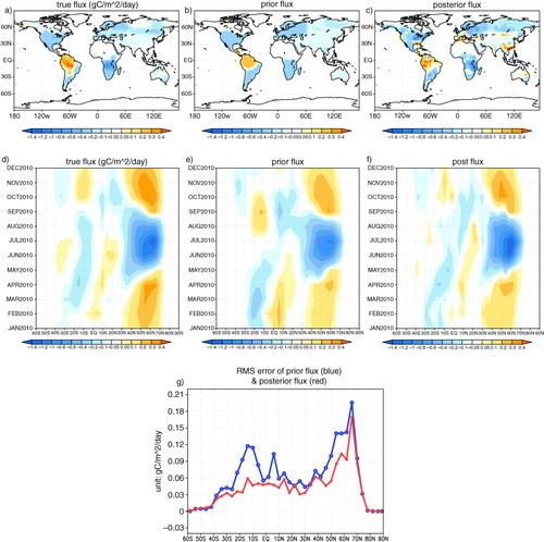
The true and the prior terrestrial biosphere fluxes have the same annual totals globally (−5.3 GtC), but they have different seasonal and diurnal cycles and spatial patterns, especially in the tropics. As shown in Fig. 1, both the seasonal and diurnal cycles of the prior flux over the Northern Hemisphere (NH) are weaker. To some extent, the difference between the prior flux used in the control inversion and the true flux reflects the current understanding of the carbon cycle: the global net flux (which is well constrained by the atmospheric CO₂ observations) is less uncertain than the spatial and temporal distribution of this net flux (Le Quere et al., 2013).

Fig. 1 The annual mean true flux (a), the prior flux (b) and the posterior flux (c) from the control inversion; the zonal mean monthly flux for the truth (d), the prior flux (e) and the posterior flux (f); RMS error of the monthly zonal mean flux for the prior (blue) and the posterior flux (g). (Unit: gC/m²/d).

2.3. Simulated ACOS-GOSAT b2.9 observations

We simulate the ACOS-GOSAT X_CO2 observations with the same observation coverage and vertical sensitivity as the ACOS-GOSAT b2.9 retrievals (O'Dell et al., 2012). GOSAT is the first successfully launched satellite that is dedicated to observe CO₂ and methane (CH₄) column abundances with the Thermal And Near Infrared Sensor for Carbon Observation-Fourier Transform Spectrometer (TANSO-FTS; Yokota et al., 2009). It started operation in February 2009, and it orbits the globe with a polar sun-synchronous trajectory. The descending orbits cross the Equator at about 13:00 local solar time. The orbits repeat every 90–100 minutes at that same local solar time. The ground track repeats every 3 d. In the near infrared, GOSAT measures sunlight reflected from the surface, and thus represents information about the entire atmospheric column that includes sensitivity to boundary layer CO₂ concentrations. Over land, TANSO-FTS points to nadir, with a 10.5-km diameter circular footprint. Over the ocean, TANSO-FTS points to the glint spot in order to compensate for the low reflectivity of the ocean in the nadir viewing direction.

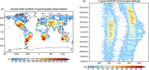
The throughput of real GOSAT retrievals is less than the full satellite coverage as a consequence of cloud contamination, poor retrieval quality, etc. In order to incorporate these effects, the simulated ACOS-GOSAT b2.9 observations are filtered according to the recommendations of the ACOS b2.9 Level 2 Standard Product Data User's Guide (available at http://oco.jpl.nasa.gov/ocodatacenter/). Only the nadir-view high-gain observations with master quality flag equal to one are simulated: the medium-gain land observations and the ocean glint data are not used. The master quality flag provided in the b2.9 retrieval product considers the confidence in the retrieved X_CO2 (see ACOS Level 2 Standard Product Data User's Guide, b2.9). Glint measurements are made exclusively over ocean and have different properties than the nadir measurements made over land (Wunch et al., 2011). The excluded medium-gain TANSO-FTS mode, which is used over bright surface scenes (e.g. over the desert) is known to have ghosting issues caused by mismatched timing delays in the signal chain (Wunch et al., 2011). The filtered observation coverage is non-uniform in both space and time (Fig. 2). A significant portion of the tropical region is not observed due to cloud contamination (Fig. 2b). The unobserved region closely follows the movement of the Inter-Tropical Convergence Zone (ITCZ). When the ITCZ moves to the northern part of the Equator during summer, so does the unobserved region. There are less than 20 observations at most of the grid points over north of the Amazon during 2010 (Fig. 2a). Over the NH high latitudes (north of 40°N), the coverage is seasonally dependent; there are no observations during late fall, winter and early spring due to the reduced signal-to-noise ratio from the low solar zenith angle. The total number of good-quality observations after filtering is 74 055 for 2010. We simulate the observations at the ACOS-GOSAT b2.9 locations without any spatial averaging. Since two observations close in space and time (i.e. observed in the same grid box within an hour) may contain the same surface flux information, some of the observations provide redundant information about surface fluxes. These redundant observations improve precision through implicit averaging in the inversion system. The amount of simulated ACOS-GOSAT observations assimilated in this study is much less than the total 330 000 GOSAT observations simulated in Chevallier et al. (2010b), which is partly because we do not simulate glint-mode GOSAT observations over ocean areas and the stricter quality control of the real retrieving process.

Fig. 2 (a) Total number of ACOS-GOSAT b2.9 good-quality observations at each 4°×5° grid point during 2010; (b) total number of daily ACOS-GOSAT b2.9 observations at each latitude as a function of time.

We generate simulated observations based on CO₂ vertical profiles, c ^t , from the nature run that is forced by the true terrestrial biosphere flux. The nature run output interval is hourly. We first sample the simulated CO₂ profiles, c ^t , at the closest times and locations of the real good-quality ACOS-GOSAT b2.9 observations. We then apply an observation operator, h(·) [eq. (1)], to calculate the model simulated X_CO2 . The model simulated X_CO2 at the i ^th location can be written as:1

where a _i is the GOSAT column averaging kernel, and and are the a priori CO₂ profile and the a priori X_CO2 assumed in the GOSAT X_CO2 retrieval process. These three quantities are from the ACOS-GOSAT b2.9 retrieval products. The simulated ACOS-GOSAT X_CO2 retrieval vector y ^o is the model simulated X_CO2 y ^t with random errors:

where the elements of vector e ^o are the random observation errors. The i ^th element of the vector y ^t is equal to . The random observation error e ^o can be rewritten as:3

where the elements of vector r are the estimated observation errors of real ACOS-GOSAT observations that comes along with the ACOS-GOSAT b2.9 retrieval products. The vector p consists of Gaussian distributed random numbers with zero mean and unity standard deviation. The observation error covariance then can be written as R=E[e ⁰(e ⁰) ^T ], where E[·] represents the expectation operator. We assume there is no error correlation among observations, so the observation error covariance R is a diagonal matrix with values ranging between 1 and 9 ppm² for most samples. The amount of observation information could be less if there were error correlations among observations, which can result from calibration errors or systematic errors in the atmospheric state, for example, surface pressure. We assume no transport errors, since we use the same transport model in both the flux inversion and the observation generation. We also ignore any systematic biases in GOSAT observations, whose impact on flux estimation has been discussed before (e.g. Baker et al., 2010; Basu et al., 2013). Therefore, the GOSAT observation impact obtained from this study is the most optimistic estimate. Neglecting these errors also allows us to focus on the fundamental role of coverage and sampling on the inference of surface CO₂ fluxes.

2.4. Flux attribution with variational data assimilation

The variational data assimilation solves for a control vector x by iteratively minimising the following cost function:4

where y ^o is the simulated ACOS-GOSAT X_CO2 defined in eq. (2). The control vector x defines temporally varying and spatially gridded scale factors, which are applied to the prior monthly mean flux, f ^b . For this application, the scale factors are monthly at each 4°×5° grid point. The prior scale vector, x ₀, is equal to one everywhere, and its error covariance matrix is B (Section 2.5). GEOS-Chem forward model M(·) simulates CO₂ vertical profiles from the surface flux x·f ^b +f ^d , where f ^d represents the 3-hourly diurnal fluxes that have zero monthly mean value at every grid point. The diurnal flux f ^d is not optimised. Based on eq. (1), the observation operator h(·) calculates the model simulated X_CO2 from CO₂ vertical profiles at the closest times and locations of ACOS-GOSAT b2.9 observations.

The optimised scale factor is the scale factor that minimises the cost function defined in eq. (4). To minimise the cost function, we use the Limited-memory Broyden–Fletcher–Goldfarb–Shanno (L-BFGS; Byrd et al., 1994; Zhu et al., 1997) numerical minimisation scheme. It is the no-bound option of the L-BFGS-B (Bounded) algorithm, that is, L-BFGS. The L-BFGS algorithm requires the gradient of the cost function5

where H is the linearised observation operator h(·), and H ^T is its adjoint. The operator M ^T is the adjoint of the GEOS-Chem model. The L-BFGS algorithm iteratively adjusts the control vector until the cost function reaches a minimum. We assess the convergence by defining a stopping criterion when the ratio between the cost function and the number of the observations is close to one. This standard is chosen in consideration of both inversion convergence (Section 3.1) and computational cost of the minimisation. In our case, a single iteration using 1 yr of data takes about 5.5 central processing unit (CPU) hours when using two quad-core processors operating at 3 GHz.

2.5. Inversion setup

In this OSSE study, we solely optimise the terrestrial biosphere flux, assuming perfect flux from the other sources and perfect initial state of CO₂. However, we consider the error propagation from non-terrestrial biosphere flux into the terrestrial biosphere flux when constructing the biosphere flux prior error statistics, which will be discussed later in this section. We choose not to optimise ocean flux, because of the sparse coverage of ACOS-GOSAT b2.9 observations over ocean (not shown). The assimilation window is 1 yr. The control vector is 12 monthly scale factors defined at each grid point. We note that the system can also estimate all types of fluxes (e.g. fossil fuel, ocean and land) at the native GEOS-Chem spatial resolution and at finer time scales.

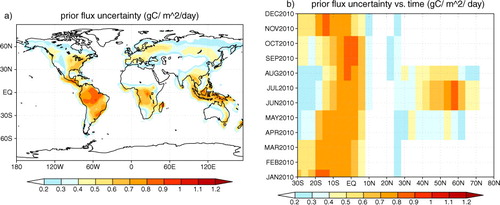
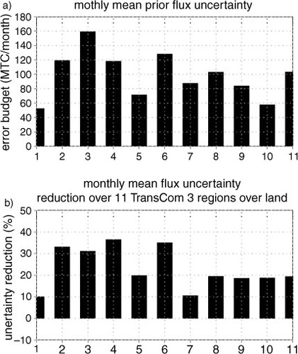
The prior flux error covariance matrix, B, is one of the key elements needed for an optimal flux estimate, and it is quite challenging to characterise (Michalak et al., 2005; Chevallier et al., 2012). In this study, the prior flux error statistics were constructed from a Monte Carlo run of CASA-GFED 3 by sampling the distributions of model parameters. The square root of the sum of the error variances over the globe for the individual fluxes has been scaled to be equal to 1.0 GtC/yr, which is the 2010 terrestrial biosphere flux uncertainty published by Global Carbon Project (http://www.globalcarbonproject.org/). This uncertainty considers the uncertainty propagation from non-biosphere fluxes (fossil fuel, land use and ocean) to biosphere fluxes. Since we estimate monthly mean flux scale factors, we scale the terrestrial biosphere flux error statistics by the absolute value of the prior monthly mean flux. We set the lower bound of the scaled errors to be 0.05 and the upper bound to be 1.0. The lower bound is to ensure that the observations can always have some impact on the surface flux estimation, since the impact of the observations is weighted against the prior error statistics [eq. (4)]. The upper bound is to avoid spuriously high values in the prior flux error statistics for the near-zero prior flux. The scaled errors change monthly at each grid point, and they are used as the square root of diagonal elements in prior error covariance matrix B. Due to the spatial inhomogeneity of the terrestrial biosphere flux and the coarse resolution of our inversion, we assume there is no spatial error correlation between different grid points. We also assume no error correlation between different months, even though the difference between the true flux and the prior flux indicates a seasonal anti-correlation, especially over the NH. Neglecting this temporal correlation will degrade the final posterior flux estimate, which we will be further discussed in Section 3.2.2. Therefore, the prior flux error covariance matrix B is diagonal. In Fig. 3, we plot the equivalent prior error statistics in flux. The magnitude of the prior flux error statistics is larger over the tropics, Eurasia and eastern North America (Fig. 3a). The tropical uncertainty is relatively high with respect to the NH uncertainty even though the NH flux is higher in absolute terms. The errors are larger during boreal summer in the NH and the whole year in the southern part of the tropical region (Fig. 3b).

Fig. 3 (a) The annual mean prior flux uncertainty (unit: gC/m²/d) calculated from the monthly flux scale factor error statistics used in the inversion; (b) the monthly zonal mean prior flux uncertainty (unit: gC/m²/d).

2.6. Posterior flux uncertainty quantification with a Monte Carlo approach

Theoretically, the posterior flux error covariance can be calculated from a number of analytical equations (e.g. Kalnay, 2003; Tarantola, 2005). However, the large dimension of the state vector x prohibits a direct calculation of this covariance. In this study, the posterior flux uncertainty is approximated using a Monte Carlo approach (Chevallier et al., 2007). In the Monte Carlo approach, an ensemble of prior states and observations are generated, consistent with the prior and observation error statistics. Then the standard deviation of the ensemble posterior fluxes gives the posterior flux uncertainty. The mean of the ensemble prior states is equal to the true flux. Different from the control inversion, the ensemble prior fluxes have the same diurnal cycle and seasonal cycle as the true flux. We performed 60 flux estimates. We chose 60 ensembles in consideration of both the computational cost and the reasonableness of the uncertainty reduction in aggregated large spatial and temporal scale.

The 60 sets of simulated observations are the ‘true’ ACOS-GOSAT with 60 different sets of random errors generated according to eq. (3). The ensemble prior fluxes are the true flux f ^t perturbed by random errors, which have the same statistics as the specified scaled prior flux error covariance B. The prior flux of the n ^th ensemble member is generated according to the following:6

where Q _n is a diagonal matrix whose elements are Gaussian distributed random numbers with zero mean and unity standard deviation.

We define the uncertainty reduction at each point as 1−σ _a /σ _b , where σ _a and σ _b are the standard deviations of the ensemble posterior and prior fluxes respectively at a specific time and location. The uncertainty reduction 1−σ _a /σ _b indicates the random error uncertainty reduction. In the later discussion, we define error as the absolute difference between the posterior flux from the control inversion and the true flux, and the uncertainty as the standard deviation of ensemble prior/posterior fluxes in the Monte Carlo flux estimation.

3. Results

In this section, we first evaluate convergence and degrees of freedom for signal (DFS). Then, we discuss the impact of assimilating simulated ACOS-GOSAT observations on CO₂ flux estimation in two aspects: 1) random error uncertainty reduction; and 2) the consequence of ACOS-GOSAT spatiotemporally biased sampling on the estimated annual flux at both the global and regional scales. Finally, through forward perturbation simulation experiments, we analyse the impact of remote CO₂ observations on flux estimation over the South American tropical region, where the observation coverage is sparse.

3.1. Convergence and DFS

In an optimal system, the minimum of the cost function is Chi-square distributed with expectation and variance equal to the number of observations. We stopped iterating after 70 iterations in the control inversion, when the ratio between the cost function and the total number of observations reaches 1.17. This indicates that the solution is close to convergence. The reason that it has not reached 1.0 yet is because the difference between the prior and the true flux is not totally random (Fig. 1) and the suboptimal prior flux error covariance. With Monte Carlo ensemble runs, where the difference between the prior and the true flux is completely random, the ratio between the cost function and the number of observations reaches 1.0 after about 20 iterations (not shown).

Given the prior information, the number of independent pieces of information that the assimilated observations provide can be described by the DFS (e.g. Rodgers, 2000). It is defined as7

where x _a is the optimised vector. DFS based on the ensemble inversions performed in the uncertainty quantification is ~1132. This indicates that the 74 055 GOSAT X_CO2 observations provide ~1132 independent observables about the fluxes given the assumed prior flux error statistics. This number is much smaller than the size of our control vector, which is 11 923 (one-third of total grid points), or 993 spatial-resolved fluxes per month. Consequently, the GOSAT X_CO2 can constrain about 10% of the spatiotemporal fluxes over the year. If we assume that the DFS is distributed evenly as a function of month, then the current system could resolve roughly 100 locations. The actual number will be higher in the NH summer and smaller in the NH winter. The DFS is still substantially higher than the number of TransCom 3 regions.

3.2. Posterior flux

3.2.1. Global flux seasonal cycle

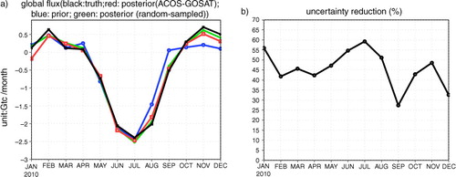
Figure 4 shows posterior flux seasonal cycle averaged over the globe (red line in Fig. 4a), and its flux uncertainty reduction as a function of month (Fig. 4b). The global averaged flux seasonal cycle has been improved (Fig. 4a), especially during the later half of the year when the prior flux (blue line) and the true flux (black line) differ the most. The monthly mean flux uncertainty reduction (Fig. 4b) is in the range of 25–60% with the reduction being largest during the boreal summer when the observation coverage is most dense. The small uncertainty reduction in December is due to two factors: sparse observation coverage over the NH high latitudes during winter and proximity to the assimilation window terminus. There are fewer observations to constrain December fluxes as opposed to, say, January fluxes where observations over the entire assimilation window can in principle provide a constraint. We can overcome the second factor by extending the assimilation window to more than 1 yr, for example, 15 months, but only analysing the flux of the first 12 months.

Fig. 4 (a) Global CO₂ flux seasonal cycle (black: the truth; blue: the prior flux; red: the posterior flux assimilating ACOS-GOSAT X_CO2 ; green: the posterior flux assimilating random-sampled X_CO2 . Unit: GtC/month). (b) Global total flux uncertainty reduction as a function of month.

3.2.2. Global annual flux and its relationship with observation sampling

In this subsection, we discuss the consequence of ACOS-GOSAT spatiotemporally biased sampling on the estimated annual flux at the global scale under the condition of our specific inversion setup. Averaged zonally, the seasonality of the posterior flux from the control inversion has been improved over all latitudes (Fig. 1f). The root mean square (RMS) error of the monthly zonal mean flux has been reduced by as much as 50% (Fig. 1g). However, the annual global total flux has become −6.0 GtC/yr after optimisation. It is worse than the prior flux (−5.3 GtC/yr), which is constructed to be equal to the true annual flux. Spatially, the annual mean flux also becomes worse over some locations, for example, over Europe (Fig. 1c). Why does the annual flux become worse while the monthly zonal mean flux is improved in all months? We find that the extra 0.7 GtC/yr sink in the annual total posterior flux is due to both the specific inversion setup and the difference between the observed value forced by the true flux and the model-predicted observations forced by the prior flux. Since the prior flux error covariance matrix is diagonal (Section 2.6), the adjustment to the prior flux during inversion would be more subject to the difference between the observations and the model simulated values than otherwise. Averaged over the globe, the annual mean simulated ACOS-GOSAT X_CO2 forced by the true flux is 387.12 ppm, and the annual mean simulated ACOS-GOSAT X_CO2 forced by the prior flux is 387.49 ppm. If we assume that an equivalent net CO₂ flux into the atmosphere is the same between a 1-ppm increase in ACOS-GOSAT X_CO2 and a 1-ppm increase in the global mean CO₂ provided NOAA (http://www.esrl.noaa.gov/), the 0.37-ppm difference is equivalent to 0.8 GtC/yr since a 1-ppm increase in global mean CO₂ is equivalent to a ~2.1276 GtC net CO₂ flux into the atmosphere (Gruber et al., 2009; Sarmiento et al., 2010). The 0.1 GtC difference from the actual posterior flux bias is because the CO₂ has not been well mixed towards the end of the year, which affects the accuracy in transferring CO₂ difference into flux. As we shall show, this 0.37-ppm difference is a consequence of the sampling of GOSAT.

In order to better understand where the 0.37-ppm difference comes from, we plot 10-d running-mean X_CO2 from the nature run sampled with different strategies in Fig. 5a. X_CO2 here is a pressure-weighted column CO₂ without using the ACOS-GOSAT averaging kernels. When only sampled at the ACOS-GOSAT locations and times (black line), the annual mean X_CO2 is 0.14 ppm smaller than the annual mean X_CO2 sampled at all grid points every 3 hours (blue line). This difference is a combination effect of ACOS-GOSAT seasonally dependent partial geographic sampling and daytime only sampling. When we sample X_CO2 at ACOS-GOSAT locations every 3 hours (red line in Fig. 5a and b), the annual mean X_CO2 is 0.05 ppm smaller than the annual mean X_CO2 sampled at all grid points every 3 hours. When only sampled at the ACOS-GOSAT observing time, the annual mean X_CO2 is 0.09 ppm smaller than the annual mean X_CO2 sampled every 3 hours, even though both strategies sample the same ACOS-GOSAT locations. It indicates that the ACOS-GOSAT daytime only sampling results in −0.09-ppm bias, while partial geographic sampling introduces −0.05-ppm bias. The low bias from the daytime only sampling is because the terrestrial biosphere absorbs CO₂ from the atmosphere during the daytime. Miller et al. (2007) show that the X_CO2 sampled at 13:00 pm (local time) is most close todaily average X_CO2 . However, the difference between X_CO2 sampled at 13:00 pm and the daily average X_CO2 depends on the magnitude and phase of terrestrial biosphere diurnal cycle. The seasonally dependent sampling introduces a low bias in X_CO2 is because of the ACOS-GOSAT preferentially samples in the NH high latitudes during summer, which is the time of significant carbon uptake from terrestrial biosphere, while having a relatively low spatial sampling yield in the late fall and winter.

Fig. 5 (a) Comparison of X_CO2 (unit: ppm) from nature run sampled with different sampling strategies. Blue: daily averaged X_CO2 sampled at every grid point every 3 hours; red: daily averaged X_CO2 sampled at the ACOS-GOSAT locations every 3 hours; black: X_CO2 sampled at the ACOS-GOSAT locations and observing time. (b) Red: the difference between X_CO2 sampled at the ACOS-GOSAT locations and the X_CO2 sampled everywhere; black: the difference between X_CO2 sampled at the ACOS-GOSAT locations and observing time and the X_CO2 sampled everywhere every 3 hours. (c) Black: the difference between the observations and the X_CO2 forced by the prior flux used in the control inversion; red: the difference between the observations and the X_CO2 forced by the flux with the same diurnal cycle as the true flux but with the same seasonal cycle as the prior flux used in the control inversion.

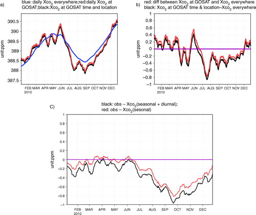
The above analysis about the nature run X_CO2 sampled with different strategies implies that two X_CO2 fields sampled at ACOS-GOSAT locations and times could have different annual mean values when the surface CO₂ fluxes have different diurnal and seasonal cycles, even with the same annual flux, as is the case here. Compared to the prior flux used in the control inversion, the true flux has a stronger seasonal cycle (Fig. 1) and diurnal cycle (not shown), especially over the NH. ACOS-GOSAT tends to sample the locations and times when the biosphere absorbs CO₂ from the atmosphere, for example, daytime and boreal summer, so the observations have a lower value than the X_CO2 forced by the prior flux when sampled at ACOS-GOSAT locations and times (black line in Fig. 5c). In order to disentangle the contribution of diurnal biased sampling from the seasonally dependent sampling, we run a CO₂ simulation, in which the terrestrial biosphere flux has the same diurnal cycle as the true flux while maintaining the same seasonal cycle as the prior flux used in the control run. The annual net flux from this combined flux is still −5.3 GtC/yr. The annual mean difference between the observations and the X_CO2 sampled at the GOSAT locations and time (red line in Fig. 5c) is −0.25 ppm, which is the combination effect of the seasonally dependent sampling and the different seasonal cycle between the true flux and the prior flux. It also implies that the diurnally biased sampling in combination of the different diurnal cycle between the true flux and the prior flux results in −0.12 ppm difference. Therefore, the 0.37-ppm difference between the simulated ACOS-GOSAT X_CO2 from the nature run and the simulated ACOS-GOSAT X_CO2 forced by the prior flux is due to the spatiotemporally dependent sampling of ACOS-GOSAT X_CO2 observations (Fig. 3) in combination with the systematic spatiotemporal difference between the true flux and the prior flux (Fig. 1).

In order to further test whether the bias in the annual total posterior flux is due to ACOS-GOSAT sampling, we did another experiment that assimilates the simulated X_CO2 observations with a random distribution in space and time, but with the same observation error statistics and sensitivity as ACOS-GOSAT X_CO2 . We find that the posterior flux (green line in Fig. 4a) from this experiment is −5.4 GtC, much closer to the true flux (−5.3 GtC) than the posterior flux with the GOSAT sampling characteristics. Compared to the posterior flux constrained by ACOS-GOSAT X_CO2 (red line in Fig. 4a), the posterior flux assimilating the random sampled X_CO2 is much more accurate during the winter months, when ACOS-GOSAT X_CO2 almost has no sampling over the high latitudes. This experiment proves that the bias in the posterior flux when assimilating the simulated ACOS-GOSAT X_CO2 is due to its spatiotemporally dependent sampling. Even with ACOS-GOSAT, including a more realistic temporal error correlation (e.g. the seasonal anti-correlation) would reduce the impact of the biased ACOS-GOSAT X_CO2 sampling and therefore the bias in the annual total flux. However, as far as we know, the current state-of-the-art inversion systems (e.g. Chevallier et al., 2007; Baker et al., 2010; Basu et al., 2013) do not have such seasonal anti-correlation error statistics, which is due to the computational cost and complexities of a large-scale inversion system. Without an accurate seasonal cycle in the prior flux or the accurate prior flux error covariance, it requires caution to interpret the annual total flux when assimilating GOSAT X_CO2 or GOSAT-type X_CO2 observations.

3.2.3. Accuracy, uncertainty reduction and biases of the posterior flux at TransCom 3 regions

In this subsection, we discuss the impact of simulated ACOS-GOSAT observations on the aggregated flux estimation at the 11 land regions (Fig. 6l) defined in TransCom 3.

Fig. 6 Flux seasonal cycle comparison among the truth (black), the prior flux (blue) and the posterior flux (red) at 11 TransCom regions over land; purple line is the total number of simulated ACOS-GOSAT observations at each region as a function of month (unit: 100, right y-axis); (a) North American Boreal; (b) North American Temperate; (c) South American Tropical; (d) South American Temperate; (e) Northern Africa; (f) Southern Africa; (g) Eurasian boreal; (h) Eurasian temperate; (i) Tropical Asia; (j) Australia; (k) Europe. On the top of each panel lists the RMS error of the prior flux (first number) and the posterior flux (second number). Unit: gC/m²/d; (l) the geographic boundaries of the 11 regions.

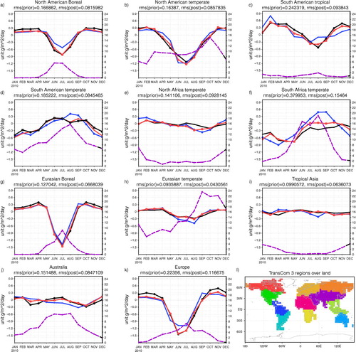
The seasonal cycle over these 11 regions has been improved (Fig. 6a–k). The RMS error reduction is between 35 and 63%, with the reduction being around 50% over most of the regions. The posterior flux (red line) and the true flux (black line) have the same seasonal cycle phase, even with a dissimilar phase in the prior flux (blue line), for example, in the tropics (Fig. 6d, f). The amplitude of the seasonal cycle has also been improved. The magnitude of error reduction has a close relationship with the number of observations assimilated (purple line in Fig. 6a–k). Over the NH boreal region (Fig. 6a, g, k), during the winter when the observations are sparse, the posterior flux error only becomes slightly smaller than the prior flux error; while during the boreal summer when the observations are dense, the posterior flux has much smaller error than the prior flux. Even though the monthly flux in all these TransCom 3 regions has been improved, the annual mean flux becomes worse over some regions. For example, over Europe, the RMS error of the monthly prior flux is 0.22 gC/m²/d, and the RMS error of the monthly posterior flux has been reduced to 0.12 gC/m²/d. However, the annual mean flux is −0.22 gC/m²/d after optimisation, while the true annual mean flux and the prior flux are −0.15 and −0.19 gC/m²/d, respectively. This degradation of the annual mean flux is due to the seasonally and diurnally biased sampling in combination with the different seasonal cycle and diurnal cycle between the prior and the true flux as discussed in Section 3.2.2. ACOS-GOSAT observations capture the stronger sink during summer, but they miss the stronger source during spring and winter in the true flux, which results in the stronger annual posterior sinks over Europe and the North American boreal region (Figs. 1c, 6a and k). Including a seasonal anti-correlation in the prior flux covariance would increase the source magnitude of the prior flux during winter and spring when ACOS-GOSAT observations are not available and, therefore, reduce the bias in the annual total flux over Europe and The North American boreal region.

The uncertainty reduction of the monthly mean flux over the TransCom 3 regions ranges from 10% over North American boreal to 38% over South American temperate (Fig. 7b). The magnitude of uncertainty reduction is related to both the prior flux error (Fig. 7a) and the observation coverage. Over North American boreal, both the total number of observations (purple line in Fig. 6f) and the prior flux error (Fig. 7a) are small, so the uncertainty reduction is small. Over the South American tropical region, even though the total number of observations is small, only 1073, the uncertainty reduction is still 30%, which is mainly due to the relatively large magnitude of the prior flux uncertainty (Fig. 7a) and the impact of remote observations (Section 3.3). Chevallier et al. (2009) showed that the fractional uncertainty reduction ranges from 25 to 80% over terrestrial TransCom 3 regions when assimilating simulated GOSAT observations without transport errors, which is larger than we find here. We speculate that the main reason is due to the difference in the number of observations assimilated (Section 2.4).

Fig. 7 Monthly mean prior flux uncertainty (a) and the uncertainty reduction at 11 TransCom regions over land (b). 1: North American Boreal; 2: North American Temperate; 3: South American Tropical; 4: South American Temperate; 5: Northern Africa; 6: Southern Africa; 7: Eurasian boreal; 8: Eurasian temperate; 9: Tropical Asia; 10: Australia; 11: Europe.

3.3. The sensitivity of remote CO₂ concentrations to the surface flux over the South American tropical region

The South American tropical region is home to one of the world's largest tropical rainforests and is experiencing rapid land-cover change (e.g. Lepers et al., 2005). Understanding the carbon budget over this region is crucial to improve our understanding of the global carbon cycle and the impact of human activity on ecosystems. However, due to the lack of observation coverage so far, the carbon budget over this region still has a large uncertainty (e.g. Stephens et al., 2007). We showed theoretically that ACOS-GOSAT could reduce the flux uncertainty by 30% even with sparse observation coverage over this region. In this subsection, through forward perturbation simulation experiment, we examine contributions to the improvement aside from the local observations.

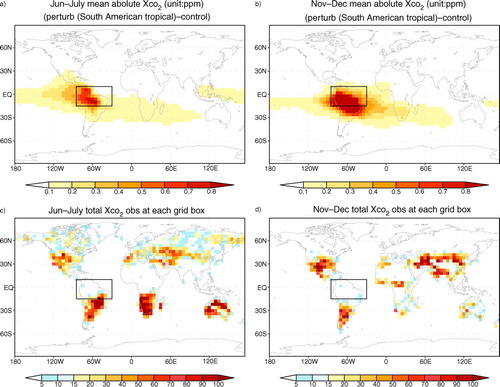
In this experiment, we perturb the prior flux in the control run over the South American tropical region (rectangle in Fig. 8) to equal the true flux in the nature run. We then compare X_CO2 from this perturbation experiment to the X_CO2 from the original control run. The perturbed region is a close approximation to the TransCom3 South American tropical region. We find that the surface CO₂ flux over the perturbed region has an impact on X_CO2 over South American temperate and South Africa (Fig. 8a and b). These regions have much denser observational coverage than over the perturbed region (Fig. 8c and d). The monthly mean X_CO2 difference between the perturbed run and the control run is about 0.2 ppm over South Africa, and the magnitude can be up to 0.8 ppm over South American temperate. The instantaneous X_CO2 difference between the perturbed run and the control run can be more than one ppm over these regions, which is significant relative to the observation error statistics (one ppm to three ppm). When the Intertropical Convergence Zone moves to the north of the Equator during boreal summer, the surface CO₂ flux over the perturbed region also has large impact on the X_CO2 over Central to North America (Fig. 8a). This experiment indicates that the X_CO2 observations over Central to North America during boreal summer and the X_CO2 observations over South African and South American temperature regions have strong sensitivities to the CO₂ flux over South American tropical region. Therefore, the posterior flux improvement over the perturbed region is mainly from the impact of the observations over these regions, since where the observation coverage is much denser than the observation coverage over the perturbed region (Figs. 1, 8c and d). In this study, we do not consider transport errors. Chevallier et al. (2010b) found that the largest bias happens in the South American tropical region when assimilating simulated GOSAT observations in the presence of transport errors. When the model is imperfect, this remote connection between flux and the X_CO2 may also lead to dipole surface CO₂ flux estimation (Stephens et al., 2007). Fig. 8a and b also show that the X_CO2 observations over the Eastern Tropical Pacific and the South Atlantic Ocean have strong sensitivities to the flux over the perturbed region. We expect that the assimilation of X_CO2 observations especially glint observations over these oceanic regions could have a significant impact on the estimate of South American tropical terrestrial biosphere flux.

Fig. 8 The time averaged absolute X_CO2 difference (unit: ppm) between the control run and a separate simulation where the surface flux is perturbed within the rectangle. The magnitude of this perturbation is equal to the difference between the control and nature run surface flux. (a) Averaged over June and July; (b) averaged over November and December. Total number of simulated ACOS-GOSAT observations at each grid cell for these two time periods. (c) June and July; (d) November and December.

4. Discussion and Conclusions

In this paper, we describe the variational inversion system developed as part of the CMS-Flux (http://www.carbon.nasa.gov, http://cmsflux.jpl.nasa.gov) and demonstrate the performance of this system in the context of an OSSE. Using the same coverage and sensitivity as the real ACOS-GOSAT b2.9 observations for 2010, we further discuss the impact of GOSAT spatiotemporally biased sampling on the net flux estimation, and the impact of remote observations on tropical flux estimation, where the GOSAT has sparse observation coverage. The results from this OSSE help us understand the impact of the unique ACOS-GOSAT spatiotemporal sampling on flux estimation. A follow-on paper will describe the assimilation of real ACOS-GOSAT observations.

With the Monte Carlo method, we quantified the random error uncertainty reduction in the posterior flux. We carried out 60-member ensemble inversions, in which the ensemble prior fluxes and the ensemble-simulated observations follow the error statistics used in the inversion. The degree of freedom for signal is ~1132, which indicates that a 1-yr of total 74 055 GOSAT X_CO2 observations has ~1132 independent quantities about the fluxes given the assumed prior flux error statistics. The results show that the uncertainty reduction of the monthly global mean flux ranges from 25 to 60%. When aggregated to TranCom3 regions, the monthly mean flux uncertainty reduction ranges from 10% over North American boreal to 38% over South American temperate, where the observation coverage is dense and the prior flux uncertainty has relatively large magnitude.

We also found that the ACOS-GOSAT observations can reduce the uncertainty over the South American tropical region by 30% in spite of the sparse local observation coverage. Through a sensitivity experiment, we illustrated that this large uncertainty reduction is mainly from the observations over Central America, South American temperate and South Africa, where the CO₂ concentrations are sensitive to South American tropical flux. Parazoo et al. (2013) show that the X_CO2 observations and Solar-induced Chlorophyll Fluorescence (SIF) from GOSAT provide complementary information about the net flux and the Gross Primary Production (GPP) over the Southern Amazonia region, which indicates that we can use these two types of observations to disentangle respiration and GPP over the broad Amazonia region.

With a control inversion, in which the prior flux has the same global annual total flux as the true flux, but has different seasonal and diurnal cycle, we assessed the consequence of ACOS-GOSAT spatiotemporally biased sampling on the estimated annual flux in both the global and regional scale when using a diagonal prior flux error covariance. ACOS-GOSAT observations sample the atmosphere during daytime and have dense observation coverage during boreal summer, so the mean X_CO2 sampled at ACOS-GOSAT observing locations and times has lower value than the mean X_CO2 sampled everywhere. Even forced by the same annual total fluxes, the global annual mean X_CO2 from the nature run is about 0.37 ppm lower than the X_CO2 forced by the prior flux when sampled at the ACOS-GOSAT locations and times. This leads to ~0.7 GtC more sink in the posterior global flux than the true flux when neglecting the temporal correlation in the prior flux error covariance. Because of the seasonally dependent sampling over the NH boreal region (e.g. Europe) and the stronger seasonal and diurnal cycle of the true flux, the posterior annual total flux over the NH boreal region also has a larger sink than the true flux. Previous studies (Corbin and Denning, 2006; Corbin et al., 2008; Parazoo et al., 2012) show that clear-sky and daytime only sampling introduces bias in the satellite X_CO2 observations. The seasonally dependent sampling has not been quantitatively discussed before. In most of the previous OSSE studies (e.g. Baker et al., 2010; Chevallier et al., 2010b), they assume no diurnal cycle in the prior flux (Baker et al., 2010) or assume the same diurnal and seasonal cycles in both the prior and the true fluxes (Chevallier et al., 2010b). The current state-of-the-art inversion systems (e.g. Chevallier et al., 2007; Baker et al., 2010; Basu et al., 2013) do not have seasonal temporal correlation in the prior flux error covariance matrix, though some inversion systems (e.g. Chevallier et al., 2010b; Yadav and Michalak, 2013) include temporal error correlations that decay exponentially with time. However, the prior fluxes used in inversions most likely have different seasonal cycle and diurnal cycle from reality. Yang et al. (2007) and Keppel-Aleks et al. (2012) both find that the seasonal cycle of CASA climatology flux, which is widely used in flux inversions, is about 30 to 40% weaker than the seasonal cycle constrained by X_CO2 . Therefore, caution is needed to interpret the global and regional annual net flux estimated from spatiotemporally biased sampling observations, such as GOSAT.

This study demonstrates the significant impact on flux estimation of assimilating simulated ACOS-GOSAT observations with the CMS flux inversion system. However, the CMS flux inversion system has some common problems with other inversion systems, and these problems require more investigation. These problems include, but are not limited to, the specification of prior flux error statistics, uncertainty quantification and the impact of transport errors.

5. Acknowledgements

We acknowledge the funding support from NASA Carbon Monitoring System program, NASA ACOS CO₂ project (D. K. Henze) and OCO-2 science team grant (11-OCO211-24). We thank four anonymous reviewers for their constructive comments. The GOSAT-ACOS X_CO2 data were produced by the ACOS/OCO-2 project at the Jet Propulsion Laboratory, California Institute of Technology, and obtained from the ACOS/OCO-2 data archive maintained at the NASA Goddard Earth Science Data and Information Services Center. The GOSAT spectra were provided to the ACOS Team through a GOSAT Research Announcement (RA) agreement between the California Institute of Technology and the three parties, JAXA, NIES and the MOE. A portion of this research was carried out at the Jet Propulsion Laboratory, California Institute of Technology, under a contract with the National Aeronautics and Space Administration.

Appendix

Validation of GEOS-Chem CO₂ adjoint model

The validation method for the CO₂ adjoint model is similar to the GEOS-Chem full chemistry adjoint model (Henze et al., 2007). The adjoint code for the CO₂ emissions and vertical transport processes is validated by comparing sensitivities calculated with the adjoint model to sensitivities calculated using finite differences. For this comparison, horizontal transport is turned off in both the forward and adjoint model (advection is discussed in more depth below), rendering the GEOS-Chem model an ensemble of column models. We then calculate the sensitivity of CO₂ concentrations at the surface of one column with respect to scaling factors applied to initial conditions in that column one month earlier. In this configuration, both finite difference and adjoint sensitivities can be evaluated simultaneously throughout the model domain. This is preferable to validating the adjoint model with horizontal transport included, in which case either thousands of model runs are required to have a set of comparable sensitivities, or the comparison is limited to a small number of arbitrarily selected locations. The slope and regression coefficients (r ²) comparing the sensitivities evaluated using adjoint versus finite difference calculations in each model column throughout the globe are 0.999 and 0.999, respectively, which confirms the accuracy of the adjoint code. Similar tests were performed to validate that the adjoint sensitivities with respect to the emissions scaling factors are also calculated correctly.

The adjoint of the horizontal advection operator in GEOS-Chem is solved using the continuous approach, wherein the sign of the winds is reversed and the same numerical solver [the second-order piecewise parabolic solver of Lin and Rood (1996)] is used in the solution of the adjoint advection equation as is used in the forward GEOS-Chem model, and the evolution of the model's pressure field is backtracked following the forward model (i.e. the continuity equation is kept as a hard constraint to enforce consistency between the forward and adjoint transport). The details were described in Henze et al. (2007), as well several other studies (Vukicevic et al., 2001; Thuburn and Haine, 2001; Hakami et al., 2007; Gou and Sandu, 2011).

References

- Andres R. J. , Gregg J. S. , Losey L. , Marland G. , Boden T. A . Monthly, global emissions of carbon dioxide from fossil fuel consumption. Tellus B. 2011; 63(3): 309–327.
- Baker D. F. , Bösch H. , Doney S. C. , O'Brien D. , Schimel D. S . Carbon source/sink information provided by column CO2 measurements from the Orbiting Carbon Observatory. Atmos. Chem. Phys. 2010; 10: 4145–4165.
- Basu S. , Guerlet S. , Butz A. , Houweling S. , Hasekamp O. , co-authors . Global CO2 fluxes estimated from GOSAT retrievals of total column CO2 . Atmos. Chem. Phys. 2013; 13: 8695–8717.
- Bowman K. , Henze D. K . Attribution of direct ozone radiative forcing to spatially resolved emissions. Geophys. Res. Lett. 2012; 39: 22704.
- Byrd R. H. , Nocedal J. , Schnabel R. B . Representations of Quasi-Newton Matrices and their use in Limited Memory Methods. Math Program. 1994; 63(4): 129–156.
- Chevallier F. , Briéon F.-M. , Rayner P. J . Contribution of the Orbiting Carbon Observatory to the estimation of CO2 sources and sinks: theoretical study in a variational data assimilation framework. J. Geophys. Res. 2007; 112: 09307.
- Chevallier F. , Feng L. , Bosch H. , Palmer P. I. , Rayner P. J . On the impact of transport model errors for the estimation of surface fluxes from GOSAT observations. Geophys. Res. Lett. 2010b; 37: 21803.
- Chevallier F. , Maksyutov S. , Bousquet P. , Breon F.-M. , Saito R. , co-authors . On the accuracy of the CO2 surface fluxes to be estimated from the GOSAT observations. Geophys. Res. Lett. 2009; 36: 19807.
- Chevallier F. , Peylin P. , Bousquet S. S. P. , Bréon F.-M. , Chédin A. , co-authors . Inferring CO2 sources and sinks from satellite observations: method and application to TOVS data. J. Geophys. Res. 2005; 110: 24309.
- Chevallier F. , Wang T. , Ciais P. , Maignan F. , Bocquet M. , co-authors . What eddy-covariance measurements tell us about prior land flux errors in CO2-flux inversion schemes. Global Biogeochem. Cycles. 2012; 26: 1021.
- Corbin K. D. , Denning A. S . Using continuous data to estimate clear-sky errors in inversions of satellite CO2 measurements. Geophys. Res. Lett. 2006; 33: 12810.
- Corbin K. D. , Denning A. S. , Lu L. , Wang J.-W. , Baker I. T . Possible representation errors in inversions of satellite CO2 retrievals. J. Geophys. Res. 2008; 113: 02301.
- Cox P. M. , Betts R. A. , Jones C. D. , Spall S. A. , Totterdell I. J . Acceleration of global warming due to carbon-cycle feedbacks in a coupled climate model. Nature. 2000; 408: 184–187.
- Crisp D. , Fisher B. M. , O'Dell C. , Frankenberg C. , Basilio R. , co-authors . The ACOS CO2 retrieval algorithm – Part II: global XCO2 data characterization. Atmos. Meas. Tech. 2012; 5: 687–707.
- Crisp D. , Miller C. E. , DeCola P. L . NASA Orbiting Carbon Observatory: measuring the column averaged carbon dioxide mole fraction from space. J. Appl. Remote Sens. 2008; 2: 023508.
- Dutkiewicz S. , Follows M. J. , Bragg J. G . Modeling the coupling of ocean ecology and biogeochemistry. Global Biogeochem. Cycles. 2009; 23: 4017.
- Follows M. J. , Dutkiewicz S . Modeling diverse communities of marine microbes. Ann Rev Mar Sci. 2011; 3(1): 427–451.
- Follows M. J. , Dutkiewicz S. , Grant S. , Chisholm S. W . Emergent biogeography of microbial communities in a model ocean. Science. 2007; 315: 1843–1846.
- Friedlingstein P. , Cox P. , Betts R. A. , Bopp L. , von Bloh W. , co-authors . Climate–carbon cycle feedback analysis: results from the C4MIP Model Intercomparison. J. Clim. 2006; 19: 3337–3353.
- Gloor M. , Sarmiento J. L. , Gruber N . What can be learned about carbon cycle climate feedbacks from the CO2 airborne fraction?. Atmos. Chem. Phys. 2010; 10: 7739–7751.
- Gou T. Y. , Sandu A . Continuous versus discrete advection adjoints in chemical data assimilation with CMAQ. Atmos Environ. 2011; 45: 4868–4881.
- Gruber N. , Gloor M. , Fletcher S. E. M. , Doney S. C. , Dutkiewicz S. , co-authors . Oceanic sources, sinks, and transport of atmospheric CO2 . Global Biogeochem. Cycles. 2009; 23: 1005.
- Gurney K. R. , Law R. M. , Denning A. S. , Rayner P. J. , Baker D. , co-authors . TransCom 3 CO2 inversion intercomparison: 1. Annual mean control results and sensitivity to transport and prior flux information. Tellus B. 2003; 55(2): 555–579.
- Hakami A. , Henze D. K. , Seinfeld J. H. , Singh K. , Sandu A. , co-authors . The adjoint of {CMAQ}. Environ. Sci. Technol. 2007; 41: 7807–7817.
- Henze D. K. , Hakami A. , Seinfeld J. H . Development of the adjoint of GEOS-Chem. Atmos. Chem. Phys. 2007; 7: 2413–2433.
- Henze D. K. , Seinfeld J. H. , Shindell D. T . Inverse modeling and mapping US air quality influences of inorganic PM2.5 precursor emissions using the adjoint of GEOS-Chem. Atmos. Chem. Phys. 2009; 9: 5877–5903.
- Kalnay E . Atmospheric Modeling, Data Assimilation and Predictability. 2003; UK: Cambridge University Press.
- Keppel-Aleks G. , Wennberg P. O. , Schneider T . Sources of variations in total column carbon dioxide. Atmos. Chem. Phys. 2011; 11: 3581–3593.
- Keppel-Aleks G. , Wennberg P. O. , Washenfelder R. A. , Wunch D. , Schneider T. , co-authors . The imprint of surface fluxes and transport on variations in total column carbon dioxide. Biogeosciences. 2012; 9: 875–891.
- Kopacz M. , Jacob D. J. , Fisher J. A. , Logan J. A. , Zhang L. , co-authors . Global estimates of CO sources with high resolution by adjoint inversion of multiple satellite datasets (MOPITT, AIRS, SCIAMACHY, TES). Atmos. Chem. Phys. 2010; 10: 855–876.
- Kopacz M. , Jacob D. J. , Henze D. K. , Heald C. L. , Streets D. G. , co-authors . Comparison of adjoint and analytical Bayesian inversion methods for constraining Asian sources of carbon monoxide using satellite (MOPITT) measurements of CO columns. J. Geophys. Res. 2009; 114 D04305.
- Lepers E. , Lambin E. F. , Janetos A. C. , Defries R. , Achard F. , co-authors. A synthesis of information on rapid land-cover change for the period 1981–2000. BioScience. 2005; 55: 115–124.
- Le Quéré C. , Andres R. J. , Boden T. , Conway T. , Houghton R. A. , co-authors . The global carbon budget 1959–2011. Earth Syst. Sci. Data. 2013; 5(1): 165–185.
- Lin S. J. , Rood R. B . Multidimensional flux-form semi-Lagrangian transport schemes. Mon. Weather Rev. 1996; 124: 2046–2070.
- Los S. O. , Collatz G. J. , Sellers P. J. , Malmstrom C. M. , Pollack N. H. , co-authors. A global 9-yr biophysical land surface dataset from NOAA AVHRR data. J. Hydrometeorol. 2000; 1: 183–199.
- Mann M. E. , Bradley R. S. , Hughes M. K . Global-scale temperature patterns and climate forcing over the past six centuries. Nature. 1998; 392: 779–787.
- Marshall J. , Adcroft A. , Hill C. , Perelman L. , Heisey C . A finite-volume, incompressible Navier Stokes model for studies of the ocean on parallel computers. J. Geophys. Res.-Atmos. 1997a; 102(C3): 5753–5766.
- Marshall J. , Hill C. , Perelman L. , Adcroft A . Hydrostatic, quasi-hydrostatic, and nonhydrostatic ocean modeling. J. Geophys. Res. 1997b; 102(C3): 5733–5752.
- Menemenlis D. , Campin J. , Heimbach P. , Hill C. , Lee T. , co-authors. ECCO2: high resolution global ocean and sea ice data synthesis. Mercator Ocean Q Newsletter. 2008; 31: 13–21.
- Menemenlis D. , Hill C. , Adcrocft A. , Campin J.-M. , Cheng B. , co-authors . NASA supercomputer improves prospects for ocean climate research. EOS. 2005; 86(9): 89, 96.
- Michalak A. M. , Hirsch A. , Bruhwiler L. , Gurney K. R. , Peters W. , co-authors . Maximum likelihood estimation of covariance parameters for Bayesian atmospheric trace gas surface flux inversions. J. Geophys. Res. 2005; 110: D24107.
- Miller C. E. , Crisp D. , Decola P. L. , Olsen S. C. , Randerson J. T. , co-authors . Precision requirements for space-based XCO2 data. J. Geophys. Res. 2007; 112: 10314.
- Mu M. , Randerson J. T. , van der Werf G. R. , Giglio L. , Kasibhatla P. , co-authors . Daily and 3-hourly variability in global fire emissions and consequences for atmospheric model predictions of carbon monoxide. J. Geophys. Res. 2010; 116: 24303.
- Nassar R. , Jones D. B. A. , Kulawik S. S. , Worden J. R. , Bowman K. W. , co-authors . Inverse modeling of CO2 sources and sinks using satellite observations of CO2 from TES and surface flask measurements. Atmos. Chem. Phys. 2011; 11: 6029–6047.
- Nassar R. , Jones D. B. A. , Suntharalingam P. , Chen J. M. , Andres R. J. , co-authors . Modeling global atmospheric CO2 with improved emission inventories and CO2 production from the oxidation of other carbon species. Geosci. Model Dev. 2010; 3: 689–716.
- O'Dell C. W. , Connor B. , Bösch H. , O'Brien D. , Frankenberg C. , co-authors . The ACOS CO2 retrieval algorithm – Part 1: description and validation against synthetic observations. Atmos. Meas. Tech. 2012; 5: 99–121.
- Olsen S. C. , Randerson J. T . Differences between surface and column atmospheric CO2 and implications for carbon cycle research. J. Geophys. Res. 2004; 109: 02301.
- Parazoo N. , Bowman K. , Frankenberg C. , Lee J.-E. , Fisher J. B. , co-authors . Interpreting seasonal changes in the carbon balance of Southern Amazonia using measurements of XCO2 and chlorophyll fluorescence from GOSAT. Geophys. Res. Lett. 2013; 40: 2829–2833.
- Parazoo N. C. , Denning A. S. , Kawa S. R. , Pawson S. , Lokupitiya R . CO2 flux estimation errors associated with moist atmospheric processes. Atmos. Chem. Phys. 2012; 12: 6405–6416.
- Randerson J. T. , Thompson M. V. , Conway T. J. , Fung I. Y. , Field C. S . The contribution of terrestrial sources and sinks to trends in the seasonal cycle of atmospheric carbon dioxide. Global Biogeochem. Cycles. 1997; 11: 535–560.
- Rienecker M. M. , Suarez M. J. , Gelaro R. , Todling R. , Bacmeister J. , co-authors . MERRA: NASA's modern-era retrospective analysis for research and applications. J. Clim. 2011; 24: 3624–3648.
- Rienecker M. M. , Suarez M. J. , Todling R. , Bacmeister J. , Takacs L. , co-authors . 2008; 92. The GEOS-5 Data Assimilation System-Documentation of versions 5.0.1 and 5.1.0, and 5.2.0 NASA Tech. Rep. Series on Global Modeling and Data Assimilation, NASA/TM-2008-104606, Vol. 27.
- Rodgers C. D . Inverse Methods for Atmospheric Sounding: Theory and Practice. 2000; 238. World Scientific Publishing, Hackensack, NJ.
- Sarmiento J. L. , Gloor M. , Gruber N. , Beaulieu C. , Jacobson A. R. , co-authors . Trends and regional distributions of land and ocean carbon sinks. Biogeosciences. 2010; 7: 2351–2367.
- Stephens B. B. , Gurney K. R. , Tans P. P. , Sweeney C. , Peters W. , co-authors . Weak northern and strong tropical land carbon uptake from vertical profiles of atmospheric CO2 . Science. 2007; 316: 1732–1735.
- Suntharalingam P. , Jacob D. J. , Palmer P. I. , Logan J. A. , Yantosca R. M. , co-authors . Improved quantification of Chinese carbon fluxes using CO2/CO correlations in Asian outflow. J. Geophys. Res. 2004; 109: D18S18.
- Takahashi T. , Sutherland S. C. , Sweeney C. , Poisson A. , Metzl N. , co-authors . Global sea-air CO2 flux based on climatological surface ocean pCO2, and seasonal biological and temperature effects. Deep-Sea Res. II. 2002; 49: 1601–1622.
- Tarantola A . Inverse Problem Theory: Methods for Data Fitting and Model Parameter Estimation. 2005. Society for Industrial and Applied Mathematics (SIAM). Philadelphia, PA, USA.
- Thuburn J. , Haine T. W. N . Adjoints of nonoscillatory advection schemes. J. Comput. Phys. 2001; 171: 616–631.
- Tucker C. J. , Pinzon J. E. , Brown M. E. , Slayback D. A. , Pak E. W. , co-authors . An extended AVHRR 8-km NDVI data set compatible with MODIS and SPOT vegetation NDVI data. Int. J. Remote Sens. 26: 4485–4498.
- van der Werf G. R. , Randerson J. T. , Collatz G. J. , Giglio L. , Kasibhatla P. S. , co-authors . Continental-scale partitioning of fire emissions during the 1997 to 2001 El Niño/La Niña period. Science. 2004; 303: 73–76.
- van der Werf G. R. , Randerson J. T. , Giglio L. , Collatz G. J. , Kasibhatla P. S. , co-authors . Interannual variability in global biomass burning emissions from 1997 to 2004. Atmos. Chem. Phys. 2006; 6: 3423–3441.
- van der Werf G. R. , Randerson J. T. , Giglio L. , Collatz G. J. , Mu M. , co-authors . Global fire emissions and the contribution of deforestation, savanna, forest, agricultural, and peat fires (1997–2009). Atmos. Chem. Phys. 2010; 10: 11707–11735.
- Vukicevic T. , Steyskal M. , Hecht M . Properties of advection algorithms in the context of variational data assimilation. Mon. Weather Rev. 2001; 129: 1221–1231.
- Wunch D. , Wennberg P. O. , Toon G. C. , Connor B. J. , Fisher B. , co-authors . A method for evaluating bias in global measurements of CO2 total columns from space. Atmos. Chem. Phys. 2011; 11: 12317–12337.
- Yadav V. , Michalak A. M . Improving computational efficiency in large linear inverse problems: an example from carbon dioxide flux estimation. Geosci. Model Dev. 2013; 6: 583–590.
- Yang Z. , Washenfelder R. A. , Keppel-Aleks G. , Krakauer N. Y. , Randerson J. T. , co-authors . New constraints on Northern Hemisphere growing season net flux. Geophys. Res. Lett. 2007; 34: L12807.
- Yokota T. , Yoshida Y. , Eguchi N. , Ota Y. , Tanaka T. , co-authors . Global concentrations of CO2 and CH4 retrieved from GOSAT: first preliminary results. SOLA. 2009; 5: 160–163.
- Zhu C. , Byrd R. H. , Lu P. , Nocedal J . L-BFGS-B: algorithm 778: L-BFGS-B, FORTRAN routines for large scale bound constrained optimization. ACM Trans. Math. Softw. 1997; 23(4): 550–560.
Appendix
Validation of GEOS-Chem CO2 adjoint model
The validation method for the CO2 adjoint model is similar to the GEOS-Chem full chemistry adjoint model (Henze et al., Citation2007). The adjoint code for the CO2 emissions and vertical transport processes is validated by comparing sensitivities calculated with the adjoint model to sensitivities calculated using finite differences. For this comparison, horizontal transport is turned off in both the forward and adjoint model (advection is discussed in more depth below), rendering the GEOS-Chem model an ensemble of column models. We then calculate the sensitivity of CO2 concentrations at the surface of one column with respect to scaling factors applied to initial conditions in that column one month earlier. In this configuration, both finite difference and adjoint sensitivities can be evaluated simultaneously throughout the model domain. This is preferable to validating the adjoint model with horizontal transport included, in which case either thousands of model runs are required to have a set of comparable sensitivities, or the comparison is limited to a small number of arbitrarily selected locations. The slope and regression coefficients (r 2) comparing the sensitivities evaluated using adjoint versus finite difference calculations in each model column throughout the globe are 0.999 and 0.999, respectively, which confirms the accuracy of the adjoint code. Similar tests were performed to validate that the adjoint sensitivities with respect to the emissions scaling factors are also calculated correctly.