Impact of aerosol on post-frontal convective clouds over Germany

Abstract

We carried out simulations with predefined and simulated aerosol distributions in order to investigate the improvement in the forecasting capabilities of an operational weather forecast model by the use of an improved aerosol representation. This study focuses on convective cumulus clouds developing after the passage of a cold front on 25 April 2008 over Germany. The northerly flow after the cold front leads to increased sea salt aerosol concentrations compared to prefrontal conditions. High aerosol number concentrations are simulated in the interactive scenario representing typically polluted conditions. Nevertheless, due to the presence of sea salt particles, effective radii of cloud droplets reach values typical of pristine clouds (between 7 µm and 13 µm) at the same time. Compared to the predefined continental and maritime aerosol scenarios, the simulated aerosol distribution leads to a significant change in cloud properties such as cloud droplet radii and number concentrations. Averaged over the domain covered by the convective cumuli clouds, we found a systematic decrease in precipitation with increasing aerosol number concentrations. Differences in cloud cover, short wave radiation and cloud top heights are buffered by systematic differences in precipitation and the related diabatic effects. Comparisons with measured precipitation show good agreement for the interactive aerosol scenario as well as for the extreme maritime aerosol scenario.

• aerosol–cloud interaction
• precipitation
• natural aerosol
• anthropogenic aerosol
• regional modelling

1. Introduction

The impact of aerosol on precipitation is still one of the least understood processes in atmospheric science (Rosenfeld et al., 2008; Levin and Cotton, 2009; IPCC, 2013). Cloud-resolving modelling studies show that aerosol can have significant impacts on dynamics, microphysics and precipitation of convective clouds (Seifert and Beheng, 2006b; van den Heever and Cotton, 2007; Flossmann and Wobrock, 2010). Key components to accurately describe convective clouds are the size distribution of aerosol (Ekman et al., 2004), the complexity of the aerosol model and the cloud microphysics model (Ekman et al., 2011; Saleeby and van den Heever, 2013).

Numerical studies of single clouds and cloud systems have shown that a change in atmospheric aerosol concentration or properties can cause changes in the precipitation rate and total precipitation amount. However, sign and magnitude of the precipitation change strongly vary between the individual studies depending on the cloud type, atmospheric conditions and simulation setup as highlighted by Khain et al. (2008). A summary of the current understanding of the impact of aerosol on the precipitation of convective clouds is given by Tao et al. (2012).

Regional scale atmospheric models are able to capture the multitude of cloud types and their interaction as well as multiple atmospheric conditions over time intervals of days to years. The outcome of recent studies is that, averaged over periods of a few days and domains of hundreds of kilometres, the net change in precipitation caused by aerosol variations is very small (Bangert et al., 2011; Morrison and Grabowski, 2011; van den Heever et al., 2011; Seifert et al., 2012).

Though the effect of aerosol on the amount of precipitation is found to be weak in regional studies, larger impacts on cloud properties and spatial patterns of precipitation can be found depending on cloud type and atmospheric conditions. For the cold season in the eastern Mediterranean aerosol is found to delay precipitation (Noppel et al., 2010). For warm-frontal clouds it was shown that different contributions of vapour deposition and riming depending on cloud condensation nuclei (CCN) number concentration lead to comparable rain production (Igel et al., 2013). For stratocumulus clouds, pollution tends to produce more but smaller cloud droplets which results in greater cloud albedo, drizzle suppression and affects also entrainment (Wood, 2012).

Studies concerning cumulus clouds however show a systematic decrease in precipitation in a polluted environment. However, aerosol impact on cloud lifetime is compensated by enhanced evaporation (Jiang et al., 2006, 2009; Xue et al., 2008).

The dependence of the aerosol effect on cloud type and atmospheric conditions can be explained by feedback processes on different scales, which buffer the impact of the aerosol on large-scale total precipitation (Stevens and Feingold, 2009). Therefore, numerical studies have to focus on populations of multiple clouds developing under specific environmental conditions using models that capture the feedback processes from the micro- to the meso-scale to obtain a robust quantification of the impact of aerosol changes on clouds and precipitation.

Because of the non-linearity of atmospheric processes and the consequent unpredictable growth of small perturbations, uncertainties in the simulation results emerge with vertical velocity and cloud water content being affected the most (Wang et al., 2012). As a consequence, quantifying the impact of aerosols on clouds and precipitation is challenging and has to be analysed in context with emerging uncertainties in the simulation results. Morrison (2012) addressed this problem using a cloud system resolving simulation of an idealised supercell storm showing that the simulated impact of aerosol on single convective clouds can be strongly affected by the non-linear growth of small perturbations. Therefore, they concluded that in order to quantify the impact of aerosol on clouds and precipitation it is crucial to use simulation domains large enough to encompass a population of clouds over their whole lifetime. A similar conclusion has also been pointed out by van den Heever et al. (2011) and Stevens and Feingold (2009).

In this study, we want to investigate the improvement in the forecasting capabilities of an operational weather forecast model by the use of an improved aerosol representation. We focus on a population of post-frontal cumulus clouds developing after the passage of a cold front over Germany in April 2008. The individual clouds develop under relatively homogeneous conditions in terms of stratification, large-scale forcing and surface conditions and are therefore an ideal case to quantify the impact of aerosols on clouds and precipitation taking the discussed requirements into account. Those post-frontal cumulus clouds develop frequently after the passage of a cold front in south-easterly direction over Germany. Their shapes, tracks and life cycles have been investigated in-depth (Weusthoff and Hauf, 2008a, 2008b). However, the role of aerosol in the formation of precipitation of post-frontal cumulus clouds has not been investigated yet.

This specific situation is of special interest for the following reasons. As the cloud top height in this situation is about 1 to 2 km warm phase processes play a major role. Furthermore, a population of similar clouds each experiencing a whole life cycle can be captured within the model study. The northerly flow leads to increased sea salt aerosol concentrations compared to pre-frontal conditions. The role of sea salt aerosol as CCN has been pointed out by several studies (Pierce and Adams, 2006; Solomos et al., 2011).

We use the comprehensive online-coupled model system COSMO-ART (Vogel et al., 2009; Bangert et al., 2012) to quantify the impact of aerosol on cloud properties and precipitation. For this purpose, we use prescribed aerosol scenarios as well as simulated aerosol including natural and anthropogenic emissions and the formation of secondary aerosol. We compare the differences between prescribed and predicted aerosol characteristics toward their impact on cloud properties and precipitation.

To address the problem of emerging uncertainties in the simulation results because of the non-linearity of atmospheric processes, we use an ensemble of simulations with randomly disturbed conditions for each aerosol scenario. To our knowledge this is the first time that the impact of aerosol on clouds and precipitation is put into context with the uncertainties in the simulation results using online-coupled simulations of aerosol and clouds on the regional scale.

Section 2 explains the model framework. Section 3 describes the simulated situation and the model setup. In Section 4, we compare the model runs with observations and quantify the impacts of the individual aerosol scenarios on cloud properties, radiation and on the aerosol–cloud radiation feedback.

We want to assess the impact of a prognostic aerosol scheme in a model setup which is close to the operationally used by German Weather Service. Especially, we address the following questions:

Are post-frontal cumuli susceptible to changes in aerosol concentrations? What is the impact of a simulated aerosol distribution on cloud properties compared to different prescribed aerosol scenarios? Does aerosol have a systematic impact on precipitation formed in post-frontal cumuli? How does the precipitation of the different simulations compare to measurements? Do aerosol differences trigger further feedback processes?

2. Model framework

Investigating aerosol–cloud interactions is a challenge that requires a comprehensive online-coupled model system. We use the model system COSMO-ART (Vogel et al., 2009) which includes an online treatment of aerosol dynamics, chemistry and transport coupled with a two-moment cloud microphysics scheme (Seifert and Beheng, 2006a, 2006b). It is based on the non-hydrostatic numeric weather prediction model COSMO of Germany's National Meteorological Service (Deutscher Wetterdienst, DWD, Baldauf et al., 2011). ART stands for Aerosol and Reactive Trace gases.

As the COSMO model is used for operational forecasts, it is continually validated for the classical meteorological variables by several European weather services. A detailed evaluation of COSMO-ART concerning aerosol and gaseous compounds is given in Knote et al. (2011).

2.1. Aerosol dynamics and chemistry

For the treatment of chemical reactions of gaseous species, RADMKA (Stockwell et al., 1990; Vogel et al., 2009) is used. Aerosol is represented by an extended version of MADEsoot (Modal Aerosol Dynamics Model for Europe, extended by soot, Riemer et al., 2003) with 11 overlapping lognormally distributed modes. Secondary organic aerosol is treated using a volatility basic set approach (Athanasopoulou et al., 2013). Three of these modes consist of mineral dust and three of sea salt (Vogel et al., 2006; Stanelle et al., 2010; Lundgren et al., 2013). As mineral dust plays only a minor role at this specific synoptic situation, it is not being considered in the model runs. An overview of the aerosol modes and their chemical composition is given in Table 1.

Table 1. Chemical composition, mean diameter, and standard deviation of the eight lognormally distributed modes used for interactive simulations in this paper

	if	ic	jf	jc	s	sa	sb	sc
Soot		✓		✓	✓
Sulphate	✓	✓	✓	✓
Ammonium	✓	✓	✓	✓
Nitrate	✓	✓	✓	✓
Organics	✓	✓	✓	✓
Water	✓	✓	✓	✓		✓	✓	✓
Sodium chloride						✓	✓	✓
Initial diameter in µm
	0.01	0.08	0.07	0.08	0.08	0.2	2	12
Standard deviation
	1.7	2	1.7	2	1.4	1.9	2	1.7

if: nucleation mode without soot; ic: nucleation mode containing soot; jf: accumulation mode without soot; jc: accumulation mode containing soot; s: soot mode; sa: sea salt fine; sb: sea salt medium; sc: sea salt coarse.

The anthropogenic emission fluxes are pre-calculated (van der Gon et al., 2010). The emission fluxes of biogenic volatile organic compounds are calculated online, based on emission factors by Steinbrecher et al. (2009) and the simulated temperature and radiation at each grid point and each time step. Sea salt emission fluxes are calculated online as a function of the wind speed and sea surface temperature.

2.2. Cloud microphysics scheme

To treat aerosol–cloud interactions in a sophisticated way, a two-moment cloud microphysics scheme (Seifert and Beheng, 2001, 2006a 2006b) is included in COSMO-ART. The scheme distinguishes six hydrometeor categories (cloud drops, cloud ice, rain, snow, graupel and hail) and represents each particle type by its respective number and mass densities. A generalised gamma size distribution is used for each hydrometeor class, where the so-called shape parameters are held constant during the simulation (Seifert et al., 2012, Table 1). For the warm-phase clouds, the scheme considers autoconversion of cloud droplets to rain, accretion of cloud droplets by rain drops, self-collection of cloud and rain droplets, break-up of rain drops and evaporation of rain drops. Condensational growth of cloud droplets is calculated with a saturation adjustment technique. For the cold-phase clouds, homogeneous and heterogeneous ice nucleation, diffusional growth of ice crystals, freezing of cloud and rain droplets, aggregation, self-collection, riming, conversion to graupel, melting, sublimation, shedding and Hallett-Mossop ice multiplication are considered. The freezing of cloud and rain drops is calculated with a classical statistical approach based on an empirical relation for the freezing probability as a function of temperature. A detailed description of the cloud microphysical processes is given in Seifert and Beheng (2006a). A statistical analysis of the aerosol–cloud interaction for three summer seasons using the microphysics scheme is presented in Seifert et al. (2012).

2.3. Aerosol activation

In order to have a direct interaction between simulated aerosol and cloud microphysics, Bangert et al. (2011, 2012) extended the cloud scheme with comprehensive parametrisations for aerosol activation and ice nucleation. For the aerosol activation, the parametrisation of Fountoukis and Nenes (2005) with the giant CCN correction of Barahona et al. (2010) is used. The activation parametrisation is based on an iterative solution of the parcel model equations and enables the simulation of the feedback between aerosol and supersaturation with respect to water during cloud formation in a comprehensive way. To resolve the impact of subgrid-scale updrafts on aerosol activation, a probability density function of updrafts is used to calculate the average aerosol activation in a grid cell (Morales and Nenes, 2010; Bangert et al., 2012).

3. Simulated situation and model setup

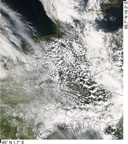
On 25 April 2008 a high-pressure ridge in 500 hPa was located over Poland and the Baltic Sea. A trough in 500 hPa lay over the North Sea and northern Germany. This caused a north-westerly flow over Germany transporting sea salt particles from the North Sea further inland. A surface low was located southwest of Iceland. An adjacent cold front passed Germany between 24 April 23 UTC and 25 April 9 UTC. After the frontal passage, cumulus clouds developed in the cold air mass (Fig. 1). The cloud bands over eastern Germany, the Czech Republic, Austria, and Switzerland are caused by the cold front, whereas the patchy clouds covering most of Germany are post-frontal convective clouds.

Fig. 1 Satellite image (true colour, MODIS-AQUA) of 25 April 2008.

As shown in previous studies (Jiang et al., 2006, 2009; Xue et al., 2008) cumulus clouds respond with systematic changes in precipitation to differences in CCN concentrations. Furthermore, using COSMO-ART we are able to capture the feedback of simulated aerosol on clouds and precipitation. Hence, we focus on these cumulus clouds as systematic differences due to aerosol concentrations are expected.

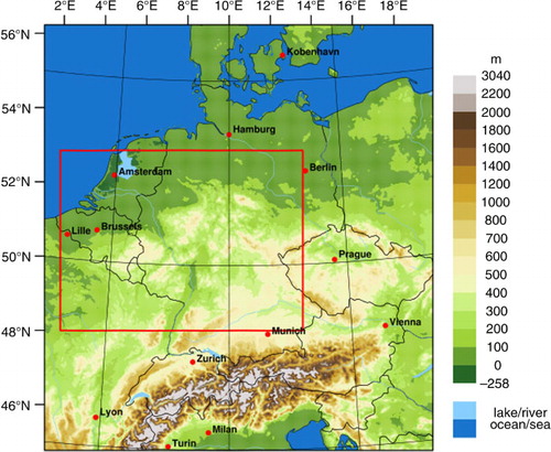
In order to capture post-frontal cumulus clouds with spatial scales on the order of 1 to 2 km correctly, a horizontal resolution much less than 1 km would be necessary. However, as we want to assess the improvement of the forecasting capabilities of an operational model through the use of an improved aerosol representation, a model setup which is close to the operational setup of German Weather Service is used. We used a horizontal grid spacing of 2.8 km and a stretched vertical grid with 50 layers up to a height of 22 km. The vertical extent of the bottom layer is about 20 m, the vertical extent of the top layer is about 1000 m. In the height of the clouds, the vertical extent of one layer is in the order of 200 m to 350 m. The integration time step is 10s. The simulation domain covers Germany and adjacent countries and is shown in Fig. 2. The domain marked by the red box is further on referred to as the convection domain and is used for analysis purposes. The convection domain is the part of the simulation domain where no frontal precipitation occurs after 9 UTC. The simulation is carried out for 25 April 2008 from 0 UTC to 21 UTC. Meteorological initial and boundary data is provided by a corresponding operational forecast model run by DWD with the same grid size. Initial and boundary data for aerosol and gases is provided by a COSMO-ART model run covering Europe with a horizontal resolution of 7 km with 2 days of spin-up.

Fig. 2 Simulation domain and model orography. The red box indicates the convection domain.

Within this study, two types of model runs were performed. First, the aerosol acting as potential CCN was horizontally and vertically homogeneously prescribed following Segal and Khain (2006). Simulations for an extreme maritime, an intermediate maritime and a continental scenario were carried out. This is a common way to account for aerosol–cloud effects in atmospheric modelling studies (Seifert et al., 2012; Igel et al., 2013). The parameters of the lognormal aerosol distributions of each scenario can be found in Table and 2 .

Table 2. The prescribed aerosol scenarios following Segal and Khain (2006)

Scenario		Parameters
Extreme maritime	N Nacl=100 cm^−3	d=0, 08 µm	σ=2, 5
Intermediate maritime	N Nacl=400 cm^−3	d=0, 08 µm	σ=2, 5
Continental	N Nacl=1700 cm^−3	d=0, 08 µm	σ=1, 68
Interactive	N=prognostic	d=diagnostic	σ=const. (mode)
	M=prognostic

N is the number density, M is the mass density, d the mean diameter and σ the standard deviation. For the prescribed scenarios the aerosol consists of sodium chloride (NaCl). For the interactive scenario the chemical composition is prognostic and σ is a constant depending on the mode.

Second, an interactive scenario using the full capabilities of COSMO-ART was performed. Aerosol mass and number densities are treated as prognostic variables. This simulated aerosol distribution acts as CCN. When running the interactive scenario, the size distribution and the chemical composition of the aerosol particles changes at each grid point and at each time step. This will be further discussed in Section 4.2. The interactive scenario increases the runtime of the prescribed scenarios by a factor of about 5.

To be consistent between the different setups aerosol in this study does not have a direct radiative effect.

3.1. Ensemble method

Because of the non-linearity of the atmospheric processes small disturbances of the atmospheric variables can grow rapidly (Lorenz, 1969; Morrison, 2012). This makes it very difficult to distil the effects of aerosol–cloud interactions on cloud formation and precipitation using numerical models or observations. Taking the results of one simulation with aerosol–cloud feedback and one simulation without aerosol–cloud feedback is not conclusive as long as there is no information on the growth of disturbances due to the remaining atmospheric processes. Small modifications of the initial state of the atmosphere can lead to similar patterns in the spatial distribution of precipitation as changes by aerosol–cloud feedback. For that reason Morrison (2012) concluded that ensemble methods are required. A variety of methods to create such ensemble is applied in operational weather forecast. Amongst them are modifications of the initial conditions, using boundary conditions from different larger scale models, modifications of the physical parametrisations and combinations of these measures.

In our study we decided to apply a method where temperature is disturbed at one single point of time. A change in temperature affects pressure and density and changes the diagnostic variables relative humidity and stratification. For this reason, temperature disturbances propagate very fast into all dynamical and physical aspects of the model system. However, it is likely that our ensemble method gives only a lower bound of the uncertainty estimation.

In order to realise the perturbations of the temperature at a single point of time at each grid point we applied the following procedure.

Two hours after the start of the simulation the time derivatives of temperature are randomly modified. The time derivative of temperature due to all physical processes (except sound waves) is averaged over all grid points in the whole model domain. This results in a mean value . Then, for each grid point, a disturbed time derivative is calculated:1

where RN is a normally distributed randomly generated number truncated at −2 and 2. The factor 100 was chosen for the following reasons. The absolute value of is much smaller than the individual time derivatives at each grid point. In order to get back to comparable values the factor 100 was chosen based on additional sensitivity studies.

For each of the scenarios with the prescribed aerosol we generated an ensemble of 23 members in order to have a sufficient number of ensemble members. For the interactive model runs we were able to calculate three ensemble members. The results of these additional model runs serve as indicators for the uncertainties caused by the non-linearity of the system and allow an improved assessment of the impact of aerosol on clouds and precipitation.

4. Discussion of the results

4.1. Post-frontal cumulus clouds properties

The following characterisations of the clouds are based on model output if not stated differently. Most of the post-frontal clouds simulated in this study consist of a warm phase and a mixed phase region. The vertical extent of the clouds is approximately from 1000 m to 3000 m above sea level, which covers approximately 10 vertical model layers (with a vertical grid spacing of about 200 m to 350 m at this height). This is exceeded by the cold phase of a limited number of clouds.

The formation of precipitation takes place within the mixed phase of the clouds. Graupel is the dominant vertically integrated precipitation. However, the surface precipitation is liquid due to melting.

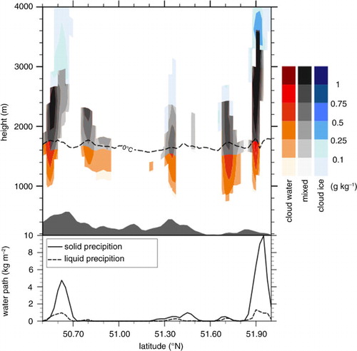
The typical vertical structures of the simulated post-frontal clouds are illustrated in Fig. 3. A population of at least five post-frontal clouds highlights the mass mixing ratios within the warm, mixed and cold phase of the clouds. Furthermore, the contribution of solid and liquid vertically integrated precipitation is shown.

Fig. 3 Top: Cross-section for cloud water and ice content greater than 0.01 g kg⁻¹ at 15 UTC. The position of the cross-section can be seen in Fig. 4b. Warm phase clouds have a red, mixed phase clouds a grey, and cold phase clouds a blue shading. The 0°C isotherm is shown as a dashed line. Bottom: Vertically integrated rain water content (dashed line) and vertically integrated snow and graupel content (solid line).

4.2. Comparison of simulated and observed radar reflectivity

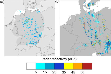
To give an impression of the horizontal distribution of the precipitation patterns, Fig. 4 shows the observed radar reflectivity at 15 UTC together with the radar reflectivity simulated within the interactive scenario. The observations cover only a limited domain indicated by the grey (above land) and white (above sea)-shaded areas, whereas the model results are presented for the entire model domain. The observed and simulated cumulus clouds developed in a band reaching from northwest to southeast Germany. The values of the simulated reflectivity are slightly overestimating the observed values. The simulated spatial patterns show similarities although differences occur in the western part of Germany where no precipitation is simulated.

Fig. 4 (a) Measured radar composite (Seifert, 2009, personal correspondence), and (b) simulated radar reflectivity in dBZ for the interactive scenario at 850 hPa on 25 April 2008 15 UTC. The observations cover only a limited domain indicated by the grey (above land) and white (above sea)-shaded areas, whereas the model results are presented for the entire model domain. The red line indicates the cross-section from Fig. 3.

4.3. Simulated aerosol properties of the interactive scenario

In contrast to the prescribed aerosol scenarios, where the chemical composition and the physical properties of the aerosol are kept constant, size distribution and chemical composition are space- and time-dependent in the interactive scenario. The temporal evolution of the simulated aerosol composition during 25 April 2008 at the altitude of the cumulus clouds (≈850 hPa) is shown in Fig. 5a. The values represent the spatial average over the convection domain given in Fig. 2. Due to the northerly flow, the mass concentration of sea salt particles increases with time. Sea salt particles account for 15% of the total aerosol mass concentration in the morning and for 25% in the evening. Whereas the increasing sea salt aerosol mass concentration is caused by the north-westerly flow, the increase of the remaining aerosol components is caused by the diurnal cycle of the emissions, the vertical mixing and by photochemical formation of secondary aerosol.

Fig. 5 (a) Temporal evolution of aerosol mass concentrations of the individual aerosol components averaged over the convection domain at the altitude of the cumulus clouds (≈850 hPa) during 25 April 2008 for the interactive scenario. (b) Corresponding total aerosol number concentration and sea salt number fraction.

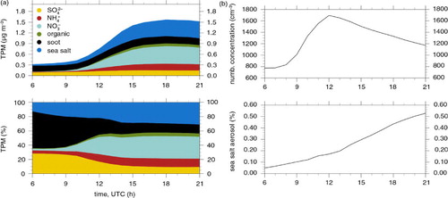
The corresponding mean total aerosol number concentration can be seen in Fig. 5b. Number concentrations of up to 1700 cm⁻³ and therefore continental conditions are reached. The decrease after 12 UTC is caused by the incipient precipitation and washout processes. The percentage fraction of sea salt aerosol increases constantly due to transport processes. However, it remains below 1%. Although sea salt has only small number concentrations compared to other aerosol, the mass fraction is, as previously shown, relatively high. Consequently, sea salt aerosol has large diameters and is therefore a very efficient CCN.

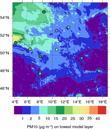
Because there are no measurements available in the cloud base regions, we validate our simulated aerosol distribution by comparing it to measured PM10 concentrations. Figure 6 shows the spatial distribution of simulated PM10 concentrations in the lowest model layer at 15 UTC and PM10 measurements which have passed the EMEP quality control (EEA, 2012). This point of time was chosen as it coincides with the maximum in precipitation. The simulated PM10 values before the passage of the front are slightly underestimated (not shown). A comparison of post-frontal values shows a reasonable agreement with measurements.

Fig. 6 Simulated PM10 concentration at 15 UTC on 25 April 2008. The model results are shaded, measured concentrations from EEA-AIRBASE EMEP stations are shown by coloured dots (EuropeanAIR quality dataBASE, http://airbase.eionet.europa.eu/).

4.4. Aerosol impact on cloud properties

In the following, we investigate the impact of the simulated aerosol on cloud properties (interactive simulation) in comparison with the prescribed aerosol scenarios. As shown in the previous section, the simulated aerosol distribution is very variable in space and time, with an increasing contribution by sea salt aerosol after the passage of the front.

Figure 7 shows a histogram of the cloud droplet number concentrations for the different scenarios. Only grid points with cloud liquid water content greater zero inside of the convection domain given in Fig. 2 between 6 UTC and 21 UTC are taken into account.

Fig. 7 Histogram of cloud droplet number concentration for grid points in the convection domain between 6 UTC and 21 UTC with cloud liquid water content greater zero.

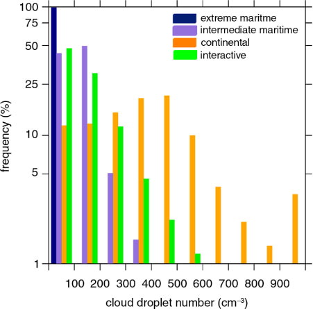
As the simulation applying the extreme maritime aerosol scenario has a number concentration of 100 cm⁻³, less than 1% of the grid points exceed cloud droplet number concentrations of 100 cm⁻³. For the intermediate maritime aerosol scenario, only a few grid points exceed 400 cm⁻³. In this case, the maximum is between 100 cm⁻³ and 200 cm⁻³. For the simulation with the continental scenario, between 3 and 4% of the cloudy grid points have cloud droplet number concentrations above 900 cm⁻³ and the maximum is further shifted to number concentrations between 400 cm⁻³ and 500 cm⁻³. Hence, each of the prescribed aerosol conditions leads to substantial differences in cloud microphysical properties.

In the interactive simulation, the simulated aerosol conditions are fundamentally different from the prescribed aerosol conditions because of the inhomogeneous spatial distribution, varying size distribution and chemical composition. Cloud droplet concentrations of up to 600 cm⁻³ are reached, which exceed the concentrations reached by applying the intermediate maritime aerosol scenario. Although the aerosol number concentrations reached in the interactive simulation are comparable to the continental aerosol scenario, only a few clouds have high (≥500 cm⁻³) cloud droplet number concentrations and most clouds have cloud droplet number concentrations comparable to the extreme maritime scenario. Further investigations have shown that in this case the spatial inhomogeneity of the aerosol number concentration has large impact on the cloud properties presented here. Additionally, a significant fraction of the simulated aerosol particles are less hygroscopic and therefore activate only at higher supersaturations than the prescribed aerosol which consists of pure sodium chloride.

The aerosol particles do not only affect the number concentration of the cloud droplets but also their effective droplet radius, which is defined as the ratio of the third to second moment of the droplet size distribution and determines the optical properties of the clouds. Moreover, the aerosol impact on the effective droplet radius is also strongly dependent on the cloud water mass concentration and therefore on the individual cloud development.

To distinguish the individual impacts of the aerosol on the cloud droplet number concentration and the effective droplet radius in the different simulations, we calculated joint histograms of cloud droplet number concentrations and effective cloud radii (Fig. 8a–d). The spatial and temporal restrictions are the same as in Fig. 7.

Fig. 8 Joint histograms of cloud properties for (a) continental, (b) intermediate maritime, (c) extreme maritime and (d) interactive scenario for grid points in the convection domain between 6 UTC and 21 UTC with cloud liquid water content greater zero.

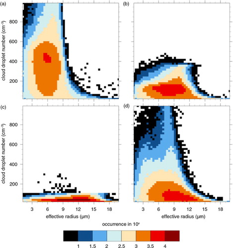
The limitations in cloud droplet number concentration for the two maritime aerosol scenarios are apparent. For the continental scenario (Fig. 8a), effective radii below 10 µm are dominating, whereas for the intermediate maritime scenario, much higher radii up to 14 µm are reached. In general, the maximum is shifted to higher radii and lower cloud droplet number concentrations from the continental to the intermediate and finally to the extreme maritime aerosol scenario, where effective radii up to 20 µm are reached. This shows that the aerosol systematically affects the microphysical properties of the post-frontal cumuli. Our results for these cumulus clouds are in keeping with the commonly assumed aerosol indirect effect showing a systematic decrease in cloud droplet radii with an increase in CCN concentrations.

The shape of the joint histogram of cloud droplet number concentrations and effective radii of the interactive scenario fits best to the continental aerosol scenario. However, the maximum lies in between the maxima of the intermediate and extreme maritime aerosol scenario. This demonstrates that in the interactive simulation, continental conditions with high aerosol and high cloud droplet number concentrations as well as maritime conditions with few cloud droplets with high effective radii are simultaneously present.

4.5. Aerosol impact on precipitation

As shown in the previous section there is a systematic impact of aerosol concentrations on cloud properties of post-frontal cumuli. When addressing the impact of aerosol on precipitation previous studies have shown only small effects averaged over time and space (Bangert et al., 2011; Morrison and Grabowski, 2011; van den Heever et al., 2011; Seifert et al., 2012). On the other hand, studies concerning cumulus clouds have shown systematic effects of aerosol concentrations on precipitation (Jiang et al., 2006, 2009; Xue et al., 2008).

Figure 9 shows the temporal evolution of the mean hourly precipitation rate within the convection domain for the interactive simulation and the simulations applying the prescribed aerosol scenarios. The spread in the curves of the individual simulations is generated as described in Section 3.1 and provides a lower bound for the uncertainty due to the non-linearity of the involved processes. Comparing the results, three different periods can be distinguished.

Fig. 9 Mean hourly precipitation rate within the convection domain of 25 April 2008 for four scenarios. The solid line is the mean value. The dashed lines indicate the standard deviation. The ensemble is generated as described in Section 3.1 and indicates the uncertainty due to the non-linearity of the atmospheric processes. As the interactive scenario has only three ensemble members, the spread is indicated by the shaded area.

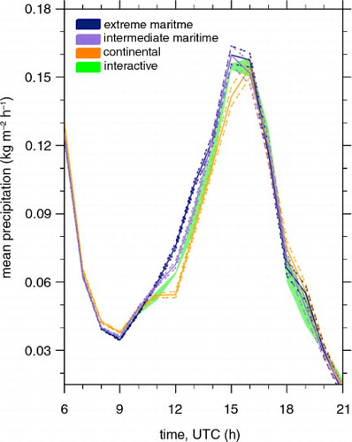
Until 10 UTC, the mean hourly precipitation rates of the four scenarios are almost identical with slightly higher rates in the simulation with the continental scenario. The precipitation during this period is still affected by the cold front itself and the difference in the precipitation rates may be attributed to a slight invigoration of the deep convective clouds associated with the front due to the higher CCN in the continental scenario as discussed in previous studies (Rosenfeld et al., 2008).

From 10 UTC to 15 UTC, the mean hourly precipitation rates differ systematically between the scenarios. During this period, the precipitation is formed exclusively in the post-frontal cumuli. The absolute difference between the simulation with the prescribed aerosol scenarios is almost constant with up to ≈0.02 kg m⁻² h⁻¹ higher precipitation rates for the extreme maritime scenario. The relative difference lies in between 4 and 28% with the maximum at 12 UTC. The mean hourly precipitation rates in the interactive simulation are in between the values of the two prescribed aerosol scenarios being closer to the results for the continental scenario most of the time.

Starting at 15 UTC, the mean hourly precipitation rates of the three simulations are again comparable. Systematic effects cannot be analysed during this period for two reasons. First, the uncertainty of the simulated precipitation rates increases, which exceeds the magnitude of the differences between the four scenarios. Second, the clouds dissipate and the formation of new clouds decreases.

In summary, there is a systematic impact of aerosol on the formation of precipitation in post-frontal cumulus clouds with an increase in precipitation by a decrease in CCN concentrations.

As shown in Section 4.1, most of the cumulus clouds are mixed phase and the formation of precipitation is dominated by graupel. Due to the model setup, only changes in CCN number concentrations and properties can eventually cause differences in precipitation. Therefore, riming may play an important role in the formation of precipitation. The collision efficiency of cloud droplets depends strongly on their diameter. The simulated mean cloud droplet diameter over all grid points with cloud water content greater zero in the extreme maritime scenario is 18.95 µm whereas in the continental scenario, a mean cloud droplet diameter of 9.91 µm is calculated. First, the mean collision efficiencies of cloud droplets on a single grid point according to eq. (64) and eq. (65) of Seifert and Beheng (2006a) were calculated. Then, we calculate the mean of overall grid points with cloud water content greater zero . is over 10 times higher for the extreme maritime scenario than for the continental scenario. As a consequence, the growth of graupel in the mixed phase via riming is more effective in the case of lower CCN concentrations. The increase in graupel mass in conjunction with the consequent increase of the fall velocity of the hydrometeors caused an increase in precipitation reaching the ground in the extreme maritime scenario. We cannot exclude that other processes play also a role in the formation of precipitation.

As described in Section 3, all simulations are driven by meteorological initial and boundary data taken from the operational forecast simulations performed at DWD. Figure 10 shows the median precipitation at 52 EOBS stations within the convection domain for the individual simulations in comparison to the median of the measured precipitation (Klok and Klein Tank, 2009). The spread represents again the uncertainty due to the non-linearity of the atmospheric processes (see Section 3.1).

Fig. 10 Median accumulated precipitation at 58 EOBS-stations (Klok and Klein Tank, 2009) within the convection domain. The red line indicates the median of the measurements. The middle line gives the ensemble mean value. The top and bottom lines indicate the standard deviation. The ensemble is generated as described in Section 3.1 and indicates the uncertainty due to the non-linearity of the atmospheric processes.

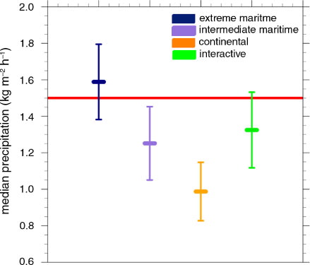
The ensemble results of the extreme maritime and the interactive scenario both cover the observed median precipitation within the standard deviation, whereas the continental and the intermediate maritime scenario both produce too few precipitation. Hence, only the extreme maritime and the interactive scenario are able to capture the precipitation amount formed by the post-frontal cumulus clouds in this situation.

At the stations, the standard deviations created by the ensembles are between 13 and 16% of the ensemble means in precipitation. Nevertheless, a clear systematic decrease in total precipitation with an increase in aerosol number concentrations can be seen.

4.6. Aerosol–cloud radiation feedback

The differences in cloud droplet number concentrations and effective radii between the individual model runs cause differences in radiation and thus have an impact on the stratification of the atmosphere. As a consequence, the stability and the convective potential of the atmosphere is changed. This has a direct impact on the initiation and intensity of the convective clouds, which is discussed in the following.

Figure 11 shows the temporal evolution of the differences in the net downward shortwave radiation (a), in the temperature in the lowest model layer (Δz≈20 m) (b), in the mean precipitation rate (c), in the cloud top height (e) and in the cloud base vertical velocity (f) of the extreme maritime and interactive simulation relative to the simulation applying the continental aerosol scenario. The mean cloud top height is calculated by the mean height of cloudy grid points below which 95% of liquid and solid atmospheric water (cloud water, rain, cloud ice, graupel and snow) is contained. To account only for warm- and mixed-phase clouds, grid points with pure ice clouds were excluded. The mean total cloud top height for each scenario is shown in Fig. 11d.

Fig. 11 Relative difference of extreme maritime scenario and interactive model run to the continental scenario in (a) net downward shortwave radiation at the surface, (b) temperatures of the lowest model layer, (c) hourly precipitation rate, (e) cloud top height, and (f) cloud base vertical velocity, (d) shows the total cloud top height. All variables are averaged over the convection domain.

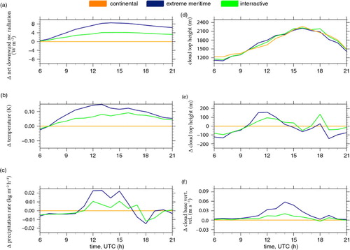
With the beginning of the convection, the mean cloud top height of the extreme maritime scenario is lower than in the continental scenario. Until 12 UTC, the growth rate in the mean cloud top height is enhanced in the extreme maritime scenario, resulting in a difference of about 160 m between the scenarios. Taking the lower mean cloud top height in the extreme maritime scenario at 6 UTC into account, the total increase till 12 UTC in the extreme maritime scenario relative to the continental scenario is about 300 m. It needs to be pointed out that these differences in mean height are in the same order as the vertical resolution of the model system.

This difference in the development of the clouds can be traced back to the fewer but larger cloud droplets (see Section 4.4) in the extreme maritime scenario. Due to the fewer but larger cloud droplets, less shortwave radiation is reflected by the clouds. In a climatological sense, this is referred to as the first indirect aerosol effect. As a result, the net downward shortwave radiation at the surface is systematically higher in the case of the extreme maritime scenario. Hence, the temperature close to the surface is also higher. As a consequence static stability decreases, which increases the convective intensity. This is consistent with the increased vertical velocity at the cloud base (Fig. 11f). In the end, this results in an increase in the mean cloud top height growth rate till 12 UTC in the extreme maritime scenario.

After 12 UTC, the difference in cloud top height between the simulations decreases again and vanishes in the afternoon. The reason for this behaviour might be the strong difference in precipitation between the simulations after 12 UTC (Fig. 11c). The more intense precipitation in the extreme maritime aerosol scenario may counteract and finally compensate the stronger convective development by the loss of cloud water mass and below cloud cooling by the evaporation of rain, which could be an explanation for the decrease of the temperature difference close to the surface between the simulations (Fig. 11b) after 13 UTC. Additionally, as there is less precipitation in the continental scenario, cloud droplets may be transported to higher levels causing convective invigoration, which can further compensate the stronger convective development of the extreme maritime scenario.

For the interactive scenario, the temporal evolution of the discussed variables shows a similar behaviour in the differences to the continental scenario (Fig. 11). The magnitudes of the differences are in most cases in between the results of the extreme maritime scenario and the continental scenario.

As shown, a change in the atmospheric aerosol alters, by its impact on the microphysical cloud structure, both the cloud optical properties and microphysical processes. In doing so, feedback processes with the state of the atmosphere are initiated, which partly counteract each other and buffer the impact of the individual processes on the cloud development.

5. Conclusion

The goal of this study is the assessment of the improvement in the forecasting capabilities of an operational weather forecast model by the use of an improved aerosol representation. In order to determine the potential range in cloud properties and precipitation changes caused by aerosol variations, we performed simulations applying three different prescribed aerosol scenarios (extreme maritime, intermediate maritime and continental) in addition to an interactive simulation where aerosol was explicitly simulated based on emissions and secondary formation.

Additionally, ensembles of 23 members for each of the prescribed and three members for the interactive scenario were carried out to separate aerosol–cloud interactions from the non-linear growth of small disturbances during simulations.

We showed that the properties of the post-frontal cumulus clouds are susceptible to changes in the aerosol, with highest cloud droplet number concentrations in the continental aerosol scenario and lowest concentrations in the extreme maritime aerosol scenario. The interactive simulation showed a variation of different cloud conditions, with average cloud droplet concentrations varying between the concentrations of the continental and extreme maritime aerosol scenarios.

The fundamentally different approaches of a fully coupled chemistry–aerosol–cloud model system in contrast to a model system using prescribed aerosol scenarios led to significant differences in cloud microphysical properties and precipitation of post-frontal cumuli.

We found a systematic increase in the hourly precipitation rate of the post-frontal cumulus clouds with a decrease in aerosol number concentration and vice versa. The maximum relative difference in the hourly mean precipitation was 28% at 12 UTC (Fig. 9). The difference in aerosol number concentration between the corresponding prescribed scenarios was 1700%.

Compared with precipitation measurements at 58 stations, the extreme maritime and the interactive scenario performed best. The standard deviations created by the ensembles were between 13 and 16% of the ensemble means in total precipitation. Nevertheless, a clear systematic decrease in total precipitation with an increase in aerosol number concentrations was found.

Cloud droplet radii differed significantly between the different scenarios. We showed that the impact of the aerosol on the cloud optical properties triggered feedback processes with an impact on the overall cloud development. Simulations with lower aerosol number concentrations showed a systematic increase in shortwave radiation at the surface causing an increase in surface temperature leading to a stronger cloud development. Finally, with a subsequent increase in precipitation in the simulation with lower aerosol number concentrations and probable convective invigoration in the polluted case, these differences diminished.

Concluding, a better representation of aerosol showed a systematic impact on the properties and precipitation of post-frontal cumulus clouds. A better representation of aerosol within an operational framework is therefore able to improve the forecasting capabilities under post-frontal conditions.

6. Acknowledgements

The authors wish to thank the following persons for their contributions to this study: Axel Seifert (DWD) for pointing out this period for further research with COSMO-ART and also for supporting us with measurements and advices. Jochen Förstner (DWD) for providing us with operational initial and boundary conditions. Andrew Ferrone (CRPGL) for preprocessing the AIRBASE data. Christoph Knote (EMPA, NCAR) for preparing the anthropogenic emission data.

The authors acknowledge the use of Rapid Response imagery from the Land Atmosphere Near-real time Capability for EOS (LANCE) system operated by the NASA/GSFC/Earth Science Data and Information System (ESDIS) with funding provided by NASA/HQ.

Finally, the authors thank our reviewers for their useful, comprehensive and very constructive comments.

References

- Athanasopoulou E. , Vogel H. , Vogel B. , Tsimpidi A. , Pandis S. , co-authors . Modeling the meteorological and chemical effects of secondary organic aerosols during an EUCAARI campaign. Atmos. Chem. Phys. 2013; 13(2): 625–645.
- Baldauf M. , Seifert A. , Förstner J. , Majewski D. , Raschendorfer M. , co-authors . Operational convective-scale numerical weather prediction with the COSMO model: description and sensitivities. Mon. Weather Rev. 2011; 139(12): 3887–3905.
- Bangert M. , Kottmeier C. , Vogel B. , Vogel H . Regional scale effects of the aerosol cloud interaction simulated with an online coupled comprehensive chemistry model. Atmos. Chem. Phys. 2011; 11(9): 4411–4423.
- Bangert M. , Nenes A. , Vogel B. , Vogel H. , Barahona D. , co-authors . Saharan dust event impacts on cloud formation and radiation over Western Europe. Atmos. Chem. Phys. 2012; 12(9): 4045–4063.
- Barahona D. , West R. E. L. , Stier P. , Romakkaniemi S. , Kokkola H. , Nenes A . Comprehensively accounting for the effect of giant CCN in cloud activation parameterizations. Atmos. Chem. Phys. 2010; 10(5): 2467–2473.
- EEA. Technical Report, European Environment Agency, Copenhagen. 2012. Online at: http://www.eea.europa.eu/data-and-maps/data/airbase-the-european-air-quality-database .
- Ekman A. , Wang C. , Wilson J. , Ström J . Explicit simulations of aerosol physics in a cloud-resolving model: a sensitivity study based on an observed convective cloud. Atmos. Chem. Phys. 2004; 4(3): 773–791.
- Ekman A. M. , Engström A. , Söderberg A . Impact of two-way aerosol-cloud interaction and changes in aerosol size distribution on simulated aerosol-induced deep convective cloud sensitivity. J. Atmos. Sci. 2011; 68(4): 685–698.
- Flossmann A. I. , Wobrock W . A review of our understanding of the aerosol–cloud interaction from the perspective of a bin resolved cloud scale modelling. Atmos. Res. 2010; 97(4): 478–497.
- Fountoukis C. , Nenes A . Continued development of a cloud droplet formation parameterization for global climate models. J. Geophys. Res.-Atmos. 2005; 110(D11): D11212.
- Igel A. L. , van den Heever S. C. , Naud C. M. , Saleeby S. M. , Posselt D. J . Sensitivity of warm-frontal processes to cloud-nucleating aerosol concentrations. J. Atmos. Sci. 2013; 70(6): 1768–1783.
- IPCC. Stocker T. F. , Qin D. , Plattner G.-K. , Tignor M. , Allen S. K. , co-authors . Climate change 2013: the physical science basis. Contribution of Working Group I to the Fifth Assessment Report of the Intergovernmental Panel on Climate Change.
- Jiang H. , Feingold G. , Koren I . Effect of aerosol on trade cumulus cloud morphology. J. Geophys. Res.-Atmos. 2009; 114(D11): D11209.
- Jiang H. , Xue H. , Teller A. , Feingold G. , Levin Z . Aerosol effects on the lifetime of shallow cumulus. Geophys. Res. Lett. 2006; 33(14): L14806.
- Khain A. P. , BenMoshe N. , Pokrovsky A . Factors determining the impact of aerosols on surface precipitation from clouds: an attempt at classification. J. Atmos. Sci. 2008; 65(6): 1721–1748.
- Klok E. J. , Klein Tank A. M. G . Updated and extended European dataset of daily climate observations. Int. J. Clim. 2009; 29(8): 1182–1191.
- Knote C. , Brunner D. , Vogel H. , Allan J. , Asmi A. , co-authors . Towards an online-coupled chemistry-climate model: evaluation of trace gases and aerosols in COSMO-ART. Geosci. Model Dev. 2011; 4(4): 1077–1102.
- Levin Z. , Cotton W. R . Aerosol Pollution Impact on Precipitation: A Scientific Review. 2009; Springer: Dordrecht. 386.
- Lorenz E. N . The predictability of a flow which possesses many scales of motion. Tellus. 1969; 21(3): 289–307.
- Lundgren K. , Vogel B. , Vogel H. , Kottmeier C . Direct radiative effects of sea salt for the Mediterranean region under conditions of low to moderate wind speeds. J. Geophys. Res.-Atmos. 2013; 118(4): 1906–1923.
- Morales R. , Nenes A . Characteristic updrafts for computing distribution-averaged cloud droplet number, autoconversion rate and effective radius. J. Geophys. Res. 2010; 115: D18220.
- Morrison H . On the robustness of aerosol effects on an idealized supercell storm simulated with a cloud system-resolving model. Atmos. Chem. Phys. 2012; 12(16): 7689–7705.
- Morrison H. , Grabowski W . Cloud-system resolving model simulations of aerosol indirect effects on tropical deep convection and its thermodynamic environment. Atmos. Chem. Phys. 2011; 11(20): 10503–10523.
- Noppel H. , Pokrovsky A. , Lynn B. , Khain A. , Beheng K . A spatial shift of precipitation from the sea to the land caused by introducing submicron soluble aerosols: numerical modeling. J. Geophys. Res.-Atmos. 2010; 115(D18): D18212.
- Pierce J. R. , Adams P. J . Global evaluation of CCN formation by direct emission of sea salt and growth of ultrafine sea salt. J. Geophys. Res.-Atmos. 2006; 111(D6): D06203.
- Riemer N. , Vogel H. , Vogel B. , Fiedler F . Modeling aerosols on the mesoscale-gamma: treatment of soot aerosol and its radiative effects. J. Geophys. Res.-Atmos. 2003; 108(D19): 4601.
- Rosenfeld D. , Lohmann U. , Raga G. B. , O'Dowd C. D. , Kulmala M. , co-authors . Flood or drought: how do aerosols affect precipitation?. Science. 2008; 321: 1309–1313. [PubMed Abstract].
- Saleeby S. M. , van den Heever S. C . Developments in the CSU-RAMS aerosol model: emissions, nucleation, regeneration, deposition, and radiation. J. Appl. Meteorol. Clim. 2013; 52(12): 2601–2622.
- Segal Y. , Khain A . Dependence of droplet concentration on aerosol conditions in different cloud types: application to droplet concentration parameterization of aerosol conditions. J. Geophys. Res.-Atmos. 2006; 111(D15): D15204.
- Seifert A. , Beheng K . A double-moment parameterization for simulating autoconversion, accretion and self collection. Atmos. Res. 2001; 59: 265–281.
- Seifert A. , Beheng K . A two-moment cloud microphysics parameterization for mixed-phase clouds. Part 1: model description. Meteorol. Atmos. Phys. 2006a; 92(1–2): 45–66.
- Seifert A. , Beheng K . A two-moment cloud microphysics parameterization for mixed-phase clouds. Part 2: maritime vs. continental deep convective storms. Meteorol. Atmos. Phys. 2006b; 92(1–2): 67–82.
- Seifert A. , Köhler C. , Beheng K. D . Aerosol-cloud-precipitation effects over Germany as simulated by a convective-scale numerical weather prediction model. Atmos. Chem. Phys. 2012; 12(7): 709–725.
- Solomos S. , Kallos G. , Kushta J. , Astitha M. , Tremback C. , co-authors . An integrated modeling study on the effects of mineral dust and sea salt particles on clouds and precipitation. Atmos. Chem. Phys. 2011; 11(2): 873–892.
- Stanelle T. , Vogel B. , Vogel H. , Bäumer D. , Kottmeier C . Feedback between dust particles and atmospheric processes over West Africa during dust episodes in March 2006 and June 2007. Atmos. Chem. Phys. 2010; 10(22): 10771–10788.
- Steinbrecher R. , Smiatek G. , Koeble R. , Seufert G. , Theloke J. , co-authors . Intra- and inter-annual variability of VOC emissions from natural and semi-natural vegetation in Europe and neighbouring countries. Atmos. Environ. 2009; 43(7): 1380–1391.
- Stevens B. , Feingold G . Untangling aerosol effects on clouds and precipitation in a buffered system. Nature. 2009; 461: 607–613. [PubMed Abstract].
- Stockwell W. R. , Middleton P. , Chang J. S. , Tang X. Y . The 2nd generation regional acid deposition model chemical mechanism for regional air-quality modeling. J. Geophys. Res.-Atmos. 1990; 95(D10): 16343–16367.
- Tao W.-K. , Chen J.-P. , Li Z. , Wang C. , Zhang C . Impact of aerosols on convective clouds and precipitation. Rev. Geophys. 2012; 50(2): RG2001.
- van den Heever S. C. , Cotton W. R . Urban aerosol impacts on downwind convective storms. J. Appl. Meteorol. Clim. 2007; 46(6): 828–850.
- van den Heever S. C. , Stephens G. L. , Wood N. B . Aerosol indirect effects on tropical convection characteristics under conditions of radiative-convective equilibrium. J. Atmos. Sci. 2011; 68(4): 699–718.
- van der Gon D. H. , Visschedijk A. , van der Brugh H. , Dröge R . A high resolution European emission data base for the year 2005, a Contribution to UBA-Projekt PAREST: Particle Reduction Strategies. 2010; Utrecht, The Netherlands: TNO. Technical Report. TNO-report TNO-034-UT-2010-01895 RPTML.
- Vogel B. , Hoose C. , Vogel H. , Kottmeier C . A model of dust transport applied to the Dead Sea Area. Meteorol. Z. 2006; 15(6): 611–624.
- Vogel B. , Vogel H. , Baeumer D. , Bangert M. , Lundgren K. , co-authors . The comprehensive model system COSMO-ART – radiative impact of aerosol on the state of the atmosphere on the regional scale. Atmos. Chem. Phys. 2009; 9(22): 8661–8680.
- Wang H. , Auligné T. , Morrison H . Impact of microphysics scheme complexity on the propagation of initial perturbations. Mon. Weather Rev. 2012; 140(7): 2287–2296.
- Weusthoff T. , Hauf T . The life cycle of convective-shower cells under post-frontal conditions. Q. J. Roy. Meteorol. Soc. 2008a; 134(633, B): 841–857.
- Weusthoff T. , Hauf T . Basic characteristics of post-frontal shower precipitation rates. Meteorol. Z. 2008b; 17(6): 793–805.
- Wood R . Stratocumulus clouds. Mon. Weather Rev. 2012; 140(8): 2373–2423.
- Xue H. , Feingold G. , Stevens B . Aerosol effects on clouds, precipitation, and the organization of shallow cumulus convection. J. Atmos. Sci. 2008; 65(2): 392–406.