Sources of variation in simulated ecosystem carbon storage capacity from the 5th Climate Model Intercomparison Project (CMIP5)

Abstract

Ecosystem carbon (C) storage strongly regulates climate-C cycle feedback and is largely determined by both C residence time and C input from net primary productivity (NPP). However, spatial patterns of ecosystem C storage and its variation have not been well quantified in earth system models (ESMs), which is essential to predict future climate change and guide model development. We intended to evaluate spatial patterns of ecosystem C storage capacity simulated by ESMs as part of the 5th Climate Model Intercomparison Project (CMIP5) and explore the sources of multi-model variation from mean residence time (MRT) and/or C inputs. Five ESMs were evaluated, including C inputs (NPP and [gross primary productivity] GPP), outputs (autotrophic/heterotrophic respiration) and pools (vegetation, litter and soil C). ESMs reasonably simulated the NPP and NPP/GPP ratio compared with Moderate Resolution Imaging Spectroradiometer (MODIS) estimates except NorESM. However, all of the models significantly underestimated ecosystem MRT, resulting in underestimation of ecosystem C storage capacity. CCSM predicted the lowest ecosystem C storage capacity (~10 kg C m⁻²) with the lowest MRT values (14 yr), while MIROC-ESM estimated the highest ecosystem C storage capacity (~36 kg C m⁻²) with the longest MRT (44 yr). Ecosystem C storage capacity varied considerably among models, with larger variation at high latitudes and in Australia, mainly resulting from the differences in the MRTs across models. Our results indicate that additional research is needed to improve post-photosynthesis C-cycle modelling, especially at high latitudes, so that ecosystem C residence time and storage capacity can be appropriately simulated.

• ecosystem C storage capacity
• ecosystem residence time
• C input
• model intercomparison
• uncertainty
• CMIP5
• net primary productivity

1. Introduction

The rising atmospheric CO₂ concentration and resultant climate warming may substantially impact the global carbon (C) budget (Solomon et al., 2007), leading to positive or negative feedback to global climate change (Friedlingstein et al., 2006; Heimann and Reichstein, 2008). Terrestrial ecosystems are estimated to have sequestered nearly 30% of the C released by anthropogenic activities from 1960 to 2008, during which fossil fuel CO₂ emissions increased from 2.4 to 8.7 Pg C yr⁻¹ (Canadell et al., 2007; Le Quere et al., 2009). However, whether the natural sink will be sustainable into the future is under debate due to the complexity of terrestrial ecosystem responses to global change, such as forest dieback (Cox et al., 2004), land use change (Strassmann et al., 2008), and storms reducing canopy photosynthesis and transferring C from plant to litter pools (Chambers et al., 2007). Therefore, it is imperative to assess the sustainability of terrestrial C storage for guiding international efforts to stabilise CO₂ concentration.

Terrestrial ecosystem C storage has been studied in the past decades using experimental (Johnston et al., 1996; Lales et al., 2001; Tang et al., 2012) and modelling approaches (Emanuel et al., 1984; Tian et al., 2012) at a biome or regional scale. For example, global climate change experiments, such as open-top chambers, free-air CO₂ enrichment (FACE) and infrared heating techniques, have been conducted to quantify responses of terrestrial C storage to elevated CO₂ (Mooney et al., 1999) and climate change (Kane and Vogel, 2009). These experimental results have advanced global model development to predict terrestrial C storage in response to climate change (Friedlingstein et al., 2006; Tian et al., 2012). Earth system models (ESMs) have often coupled atmosphere–ocean general circulation models (GCMs) with the Dynamic Global Vegetation Models (DGVMs) or Terrestrial Biogeochemistry Models (TBMs, e.g. Krinner et al., 2005; Prentice et al., 2007). The different coupled models could result in diverse results (Ahlström et al., 2013) with considerable uncertainty in magnitude and even in direction (Friedlingstein et al., 2006). The accuracy of these ESMs in simulating ecosystem C storage remains unclear, considerably affecting our confidence in predicting C storage in terrestrial ecosystem under future climate conditions.

The C storage of an ecosystem under given environmental conditions will ultimately approach its steady state (referred to as ecosystem C storage capacity, Xia et al., 2013). Ecosystem C storage capacity is often determined by C influx and mean residence time (MRT; Luo et al., 2001, 2003), as adopted in most biogeochemical models (Parton et al., 1988). Since biogeochemical models are usually first initialised to the steady state before being used for further analysis, the steady-state ecosystem C storage and its determinants are good indicators for model performance at a given C-cycle model structure. In ESMs, net primary productivity (NPP) is often estimated by canopy-absorbed photosynthetically active radiation (PAR, Cramer and Field, 1999), while MRT is calculated with photosynthate allocation or C transfer coefficients among various C pools and environmental forcing (Xia et al., 2013). The large variations on NPP and MRT among the models may result from differences in simplifying assumptions and the environmental variables used, leading to various results for terrestrial C storage capacity. A recent analysis of the 5th Climate Model Intercomparison Project (CMIP5) from Todd-Brown et al. (2013) indicated that the estimates of the global soil C pool varied 5.9-fold among 12 models, with 2.6-fold variation in NPP and 3.6-fold variation in MRT. However, spatial variations in ecosystem C storage capacity determined by NPP and MRT and multi-model variations at a global scale have not yet been well quantified.

Variations associated with regional and global NPP have been widely evaluated via comparison with data sets and among models (Kicklighter et al., 1999; Pinsonneault et al., 2011; Wang et al., 2011). For example, comparison among 17 uncoupled terrestrial biogeochemical models showed similar estimates of NPP over large areas (Cramer et al., 1999). Researchers have also analysed the sources of uncertainty in NPP via direct comparison of model structure (Adams et al., 2004) or analysis of the relationship between NPP and climate variables (Wang et al., 2011). The results showed general agreement on average among models but exhibited significant differences in spatial patterns. However, the sources of these variations in the spatial distribution of NPP remain unclear.

Mean MRT has been estimated at a global scale through soil respiration measurement (Raich and Schlesinger, 1992) and C isotope tracing (Ciais et al., 1999; Randerson et al., 1999), as well as by inverse methods at a regional scale (Barrett, 2002; Zhou and Luo, 2008; Zhao and Running, 2010). However, spatial pattern of MRT at a global scale is still unknown, limiting accurate evaluation of the terrestrial C balance and model prediction of future global C cycling in response to climate change. If uncertainties in the MRT estimation are not adequately addressed at the global scale, ecosystem C storage capacity cannot be fully understood. For example, Zhou and Luo (2008) and Zhou et al. (2012) calculated ecosystem C uptake with increased NPP and MRT in the USA and found that MRT was the key source of uncertainty in the results. Therefore, quantifying variation in NPP and MRT at a global scale is necessary for better understanding of terrestrial ecosystem C storage. To date, no studies have been conducted to examine the spatial patterns in modelled and observed ecosystem C storage capacity and their variations at a global scale.

In this study, we examined spatial patterns of ecosystem C storage capacity simulated by the ESMs included in CMIP5, evaluated the multi-model variations and explored their potential sources such as MRT, C inputs, or both. We aimed to (1) quantify spatial patterns of ecosystem C storage capacity and their multi-model variations and (2) examine the sources of variations from NPP and MRT estimates by ESMs. Here, the simulated results from five models were used to estimate MRT using C pools and influx or efflux. We mainly focused on assessing spatial variability across the models through model intercomparison at grid and global scales.

2. Materials and methods

2.1. Model description

To calculate ecosystem C storage capacity and MRT, the simulated results of ESMs from the 5th CMIP5 were used, including C influx [gross primary productivity (GPP) and NPP], respiration [autotrophic respiration (R_a) and heterotrophic respiration (R_h)] and C pools (soil, litter and plant C, http://pcmdi9.llnl.gov/esgf-web-fe/). Eight models from five institutes were available in CMIP5 (Table 1). Models from the same climate centre showed more than 90% relative similarity (e.g. MIROC-ESM base model and CHEM, NorESM1-M and ME). Therefore, the modelled results from the same centre were pooled together prior to further analysis. However, IPSL models were still retained because of the different R_e/GPP ratio between IPSL-CM5B and IPSL-CM5A with the values of 1 and 1.96, respectively. These ESMs combine climate models, atmospheric and oceanic process models, and terrestrial ecosystem models to examine the responses of earth system to global climate change. In this study, we focused on the terrestrial ecosystem models.

Table 1. Full summary of land biogeochemistry models used by ESMs

Model name	Land model	Spatial resolution	Dynamic vegetation	Fire	N cycle	LUC
CanESM 2.2	CTEM/CLASS	2.85°×2.77°	N	Y	N	Y
CCSM4.2	CLM 4.0	1.25°×0.94°	N	Y	Y	Y
IPSL-CM5A-LR	ORCHIDEE	3.75°×1.89°	N	Y	N	Y
IPSL-CM5B-LR
MIROC-ESM	MATSIRO/SEIB-DGVM	2.81°×2.79°	Y	N	N	Y
MIROC-ESM-CHEM
NorESM1-M	CLM 4.0	2.5°×1.89°	N	Y	Y	Y
NorESM1-ME

Ecosystem MRT cannot directly be obtained from ESMs’ results and is calculated by the C residence times and C allocation coefficients for individual C pools in plants and soils (Barrett, 2002). Carbon enters into the terrestrial ecosystem through plant photosynthesis, which is partitioned into various plant pools (i.e. leaf, root and woody biomass). Plant materials then die to form litter pools (i.e. metabolic, structural and coarse woody debris). The litter C is partially decomposed by microbes to release CO₂ and partially converted to soil organic matter (SOM) in fast, slow and passive pools. Most of the models share similar structures for C inputs and partition into plant or soil pools and terrestrial decomposition, but different parameters in C transfer coefficients between pools as well as their response to environmental variables could result in different MRTs across the models (Xia et al., 2013).

Carbon input or GPP is similarly simulated with the leaf-level photosynthesis model involving sunlit and shaded leaves to scale up to the region or globe with leaf area index (LAI). Among five models, different plant functional types (PFTs) were defined, which included characteristic of different climate zones or biomes, such as 9 PFTs for CanESM, 13 for IPSL and MIROC and 15 for CCSM/NorESM. However, only the MIROC model considers the vegetation dynamic (Watanabe et al., 2011).

Autotrophic respiration (R_a) is critical to estimate NPP (GPP-R_a), which includes maintenance respiration (MR) and growth respiration (GR). MIROC and CanESM simulated R_a by the respiration rate, the chemical composition of each of the plant tissues, and air temperature with a Q₁₀ function (Arora et al., 2011; Watanabe et al., 2011). While CCSM and NorESM estimated MR as a function of temperature and live tissue N concentration and GR as 0.3 times the total C in new growth (woody and non-woody tissues) for a given time step (Lawrence et al., 2011). IPSL simulated MR as a linear function of biomass and temperature, and GR is a fixed part of allocated photosynthates (30%, Piao et al., 2010).

Heterotrophic respiration or terrestrial decomposition across all ESMs is relatively uniform with a first-order decay process through 1–9 dead C pools (Todd-Brown et al., 2013). Decomposition in most models depends on Q₁₀ function or Arrhenius-type equations, which are functionally similar (Davidson and Janssens, 2006). The decomposition rate is modified as a function of temperature (T) relative to a baseline (T₀), such that F (T)=Q₁₀ ^{(T − T₀ )/10} with different Q₁₀ values across models. All models account for land use change, but Only CCSM and NorESM have the nitrogen cycle coupled with the C cycle.

2.2. Methods

MRT is the average time that a C atom remains in a compartment of the system (Luo et al., 2003). Ecosystem MRT is aggregated from C residence time in the individual plant and soil pools with different ways (Zhou et al., 2012). Zhou and Luo (2008) used the inverse model to estimate the MRT in the USA, defining MRT as the inverse of the C transfer coefficients for individual pools. Friedlingstein et al. (2006) directly estimated the MRT of dead C (litter plus soil C pools) as the ratio of total dead C to R_h. Different mean C residence times in the individual C pools probably caused regional discrepancy in ecosystem MRT. Here, we estimated ecosystem MRT using the C balance method by the ratio of the C pool to C outflow. For an ecosystem, the C pool (C_pool) has three components—vegetation, litter and soil—and C loss is ecosystem respiration (R_e), which includes R_a and R_h. Although C losses by wildfires are attributed to a large amount of C effluxes (about 2–4 Pg C yr⁻¹, about 3–6% of soil respiration, Bowman et al., 2009; van der Werf et al., 2010), it is difficult to quantify fire effects on MRT and then ecosystem C storage by both modelling and experiments. Moreover, MIROC models did not consider fire. We thus did not take fire effects into account and calculated ecosystem MRT as follows:1

At the steady state, R_e is equal to GPP. Except in IPSL-CM5A, the R_e/GPP ratios for all of the models range from 1.1 to 0.99 for the years 1850–1860, during which most of the models can be considered to be at steady state. Here, we just used IPSL-CM5B to estimate MRTs and the resultant ecosystem C storage for IPSL because IPSL-CM5A was not at the steady state. In addition, Thompson and Randerson (1999) indicated that there were two types of MRTs for terrestrial ecosystems: the GPP-based or the NPP-based MRT. The latter does not include autotrophic respiration. If not specified, ecosystem MRT refers to the GPP-based MRT in this study. To make better comparison, we also estimated the NPP-based MRT. The NPP-based MRT (MRT_cor) was corrected from ecosystem MRT with the NPP/GPP ratio.

NPP and ecosystem respiration have significant seasonal and inter-annual variability. To decrease the effects of inter-annual variability on the MRT, monthly means for all variables from 1850 to 1860 were determined for each grid cell to generate an overall mean for calculating MRT at the steady state. All of the data were regridded using R software to a common projection (WGS 84) and 1°×1° spatial resolution. Latitudinal patterns were extracted by moving averages over 1° latitudinal bands. The regridding approach assumed conservation of mass that a latitudinal degree was proportional to distance for the close grid cells (Todd-Brown et al., 2013).

Multi-model variability on NPP, MRT and terrestrial C storage capacity were measured using the standard deviation (SD) and coefficient of variation (CV=SD/mean). The SD and CV were calculated using the five models’ results for each grid at a spatial resolution of 1°×1°.

2.3. Data sets

Four data sets were used to evaluate model performance, including the NPP and NPP/GPP ratio derived from Moderate Resolution Imaging Spectroradiometer (MODIS) data (Zhang et al., 2009; Zhao and Running, 2010), the MRT for the USA estimated using the inverse model (Zhou and Luo, 2008; Zhou et al., 2012) and soil C storage from the Harmonized World Soil Database (HWSD).

We used the 0.008°×0.008° gridded MODIS product MOD17A3 from 2000 to 2009 (Zhao and Running, 2010). Here, the GPP was calculated as GPP=ɛ×FPAR×PAR, where ɛ is the radiation use efficiency of the vegetation determined by maximum ɛ in each biome (ɛ_max), temperature (T) and soil moisture (M, ɛ=ɛ_max×f (T)×f (M)). FPAR was the fraction of incident PAR, absorbed by the canopy. The annual NPP was calculated as . Here, PsnNet=GPP − R_ml − R_mr; R_ml, R_mr and R_mo are MR by leaves, fine roots and other living parts, respectively. R_g is GR. All the respiration data were obtained from the C4 MOD17 Biome Parameter Look-Up Table (BPLUT). The NPP/GPP ratio was also used to assess model performance due to its greater stability compared to the NPP or GPP alone (Zhang et al., 2009). The simulated NPPs and NPP/GPP ratios in 1995–2005 were used for model-data comparison.

Spatial patterns of directly observed MRTs are not available at the global scale for evaluating the models. Currently, regional MRTs have been estimated using inverse analysis only for the USA and Australia (Barrett, 2002; Zhou and Luo, 2008; Zhou et al., 2012). In the conterminous USA, the estimated MRTs were estimated by genetic algorithm (Zhou and Luo, 2008) and Markov Chain Monte Carlo (MCMC, Zhou et al., 2012) with values of 46 and 56.8 yr, respectively. However, MRTs estimated by Zhou et al. (2012) and Zhou and Luo (2008) were NPP-based values, so the modelled MRT_cor in the USA from 1850 to 1860 were used for data-model comparison at the grid scale. Mean MRT in Australia (Barrett, 2002) was larger than global C turnover estimates (26–60 yr), and therefore spatial patterns were not discussed.

Ecosystem C storage is composed of C pools in vegetation, litter and soil. As the largest terrestrial C pool, soil C storage was used to assess model performance for ecosystem C storage with the HWSD (FAO/IIASA/ISRIC/ISSCAS/JRC, 2012). For the HWSD, the major sources of uncertainty are related to analytical measurement of soil carbon, variation in carbon content within a soil type and assumption that soil types can be used to extrapolate soil C data. Analytical measurements of soil C concentrations are generally accurate, but measurements of soil bulk density are more uncertain (Todd-Brown et al. 2013). Therefore, we used SOC from HWSD by the amendments of typological data and a bulk density (Hiederer and Köchy, 2011) to conduct data-model comparison, with the global total of 1417 Pg C at the 30 arc second grid (http://eusoils.jrc.ec.europa.eu).

One limitation of the above datasets is that their uncertainties are poorly quantified. Here, 50 000 and 500 simulations calculated the global or regional means, respectively, through MCMC sampling with size of 5000 and 500 in R software. For each variable, the confidence interval was estimated as the 2.5 and 97.5 percentile of mean values of the 5000 (or 500) simulations. Therefore, the global mean was 0.55 (0.54–0.56) kg C m⁻² yr⁻¹ for MODIS NPP, 12.42 (12.37–12.48) kg C m⁻² for HWSD soil C, 0.53 (0.52–0.54) for the NPP/GPP ratio and 52.1 (51.6–52.6) years for MRT in the United States. This method was also used to calculate the global mean of each variable in each model.

3. Results

3.1. Ecosystem carbon storage capacity

The ecosystem C storage capacity was calculated from the sums of C storage in plant, litter and soil pools at the steady state, represented by NPP×MRT_cor. The average ecosystem C storage capacity for all five models was about 20 kg C m⁻², with a maximum of nearly 36 kg C m⁻² for MIROC and a minimum of nearly 10 kg C m⁻² for CCSM (Figs. 1 and 2). The ecosystem C storage capacity for CanESM was higher than that for IPSL due to a longer MRT_cor, although NPP in IPSL was larger than that in CanESM. The largest ecosystem C storage capacity (MIROC) was associated with the longest MRT_cor (88 yr) and a mid-range NPP (0.45 kg C m⁻² yr⁻¹). However, the lowest NPP and longest MRT_cor (NorESM) resulted in the larger ecosystem C storage capacity than that in CCSM.

Fig. 1 The spatial pattern of ecosystem C storage capacity (NPP*MRT_cor, kg C m⁻²) for the five models (modelled time: 1850–1860). Coefficient of variation (CV) was calculated for each grid cell using five models’ results.

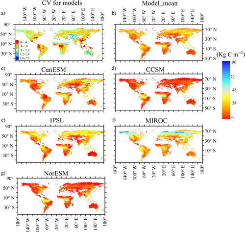
Fig. 2 The relationship between mean residence time (MRT, years) and net primary production (NPP, kg C m⁻² yr⁻¹) and the latitude pattern of ecosystem C storage capacity (NPP*MRT_cor) for five models (modelled time: 1850–1860).

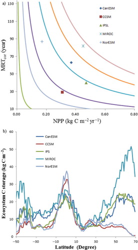
The spatial and latitudinal patterns of NPP and MRT substantially affected the patterns of ecosystem C storage capacity (Fig. 2). Between 30°S and 30°N, all five models closely simulated ecosystem C storage capacity, with similar values of NPP and MRT (Fig. 2). However, ecosystem C storage capacity for MIROC was higher at other latitudes than those for the other models, reaching a maximum at around 70°N (~55 kg C m⁻²) (Fig. 2b). The ecosystem C storage capacities for CCSM and NorESM were much lower than those for the other models, particularly at 50–30°S and 30–70°N, but relatively high at 5°S–5°S. Ecosystem C storage capacity for the NorESM was higher than that for CCSM due to a higher MRT, although they had the same terrestrial ecosystem model (CLM).

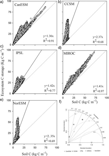
Soil C storage accounted for a large amount of ecosystem C storage (40% for CCSM and NorESM and 70% for CanESM, IPSL and MIROC, Fig. 3) and explained much of the spatial variation in ecosystem C storage across models (R ²>0.7), especially for CanESM and MIROC. However, not all of the models accurately predicted soil C storage (Fig. 3f). Across all common grid cells, the Pearson correlation coefficients between soil C data from the models and HWSD ranged from 0.06 to 0.49 and the root mean square errors (RMSE) were from 10 to 15 kg C m⁻².

Fig. 3 The relationship between ecosystem C storage and soil C across models (a, b, c, d, e) and Taylor diagram for soil C storage at grid scale (f).

3.2. NPP and NPP/GPP ratio

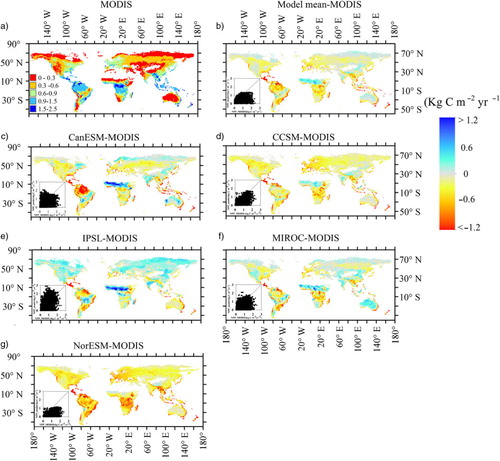
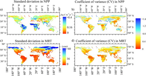
The average NPP among the five models was 0.36 kg C m⁻² yr⁻¹ from 1850 to 1860 and 0.41 kg C m⁻² yr⁻¹ from 1996 to 2005 (Table 3). Apart from NorESM, the predicted global average NPPs were close to the MODIS-based estimates with the similar latitude patterns (Fig. 7a), but there was regional variability among models (Figs. 4, 9a, b). For example, NorESM and CCSM4 underestimated NPPs for all grids except in certain tropical regions (Fig. 4d and h). CanESM and IPSL greatly underestimated NPPs for northern North America, but overestimated NPPs for northern Africa. Thus, high spatial variability across models led to high CV at most areas with the values larger than 0.5 (Fig. 9b). The highest CV occurred in high latitude and sparse vegetation regions. The SD was larger for high NPP areas and smaller where the NPP was low. The highest SDs occurred in tropical zones, while the coefficient of variance was lower than 0.1.

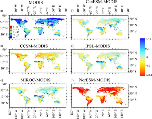
Fig. 4 Spatial pattern of net primary production (NPP, kg C m⁻² yr⁻¹) estimated from MODIS and the difference between five models and MODIS (modelled time: 1995–2005).

Apart from NorESM, all of the models estimated an average NPP/GPP ratio near to 0.5 (Table 3), although there was poor agreement between modelled ratio and the MODIS estimates at the grid cells (R ²<0.25, Fig. 5). At most areas, CanESM, IPSL and MIROC closely estimated the NPP/GPP ratios, differing by −0.05 to 0.05 from MODIS, while CCSM and NorESM greatly underestimated the NPP/GPP ratio. The latitudinal patterns of the NPP/GPP ratios for the other models were not consistent and were highly complex (Fig. 7b). For example, the NPP/GPP ratio predicted by CanESM had a series of peaks within 10°S–10°N, with the highest nearly at the equator, while the NPP/GPP ratios for the other models had lower values at these latitudes.

Fig. 5 Spatial pattern of the NPP/GPP ratio estimated from MODIS and the difference between five models and MODIS (modelled time: 1995–2005).

3.3. Mean residence time

Ecosystem MRTs at the grid scale were highly heterogeneous, ranging from 0 to thousands of years. MRT values for the majority of the grids were 5–40 yr, with the lowest values in the tropics and the highest values at high latitudes (Fig. 6). The mean MRT for all models was ~28 yr, ranging from 15 yr for CCSM to 45 yr for MIROC (Table 2). Large MRT differences occurred among the models (Fig. 6). Compared with the mean value across all models, CCSM and NorESM underestimated MRTs in most areas at <30 yr, with only 5% of the grids >50 yr. MIROC overestimated MRTs for all grids, with a majority of the MRTs <70 yr and a maximum value >568 yr.

Fig. 6 Spatial pattern of average mean residence time (MRT, years) of ecosystem for five models and the difference between five models and the average of models (modelled time: 1850–1865).

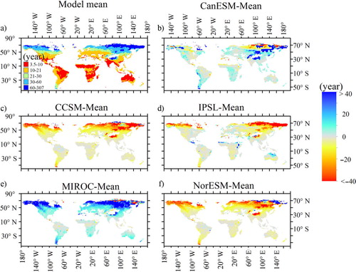
Table 2. Effects of extreme data on ecosystem mean residence time (MRT) and the publication-based global average

Model	Mean_orig (years)	Percent* eliminated data	Mean_corrected* (years)	Reference
CanESM	36.4	0	36.4
CCSM	23.02	0.8	14.5
IPSL	33.41	0.4	21.3
MIROC	132.63	0.5	44.6
NorESM1	23.02	0.07	18.0
Based on soil respiration measurement			32	Raich and Schlesinger (1992)
Based on ^13C measurement			29	Randerson et al. (1999)
			44	Ciais et al. (1999)
Models			37–60	Meyer et al. (1999)

*A majority of MRTs at all grids for all models at the same spatial resolution are less than 400 yr, so we set the threshold of 1000 yr according as the hist. of data. The percentage of the eliminated data is not more than 1% (the valid data).

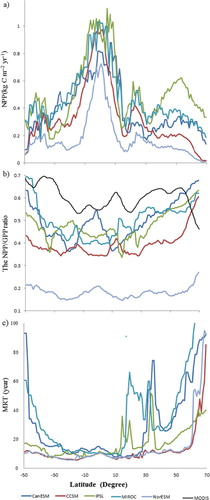
We sampled the mean MRT for each latitudinal zone at 1° intervals between 50°S and 70°N to explore latitudinal patterns in the MRT (Fig. 7). The MRTs predicted by the five models at 25°S–10°N were relatively low with low variability. The models predicted high MRTs at high latitudes because of the relatively low temperatures and lower rates of decomposition. The MRTs for CCSM and NorESM were lower than those of the other models but had similar latitudinal patterns. The MRTs for MIROC were higher than that for the other models at most latitudes, particularly at 12°N–30°N. Thus, there was high spatial variability in the MRT across models. The CV of the MRTs estimated by all five models mainly ranged between 0.2 and 0.8, with the lowest values in latitude 10°S–10°N and the largest values in the high latitude and sparse vegetation regions.

Fig. 7 The latitude pattern of NPP, the NPP/GPP ratio and mean residence time (MRT) for five models (each point representing the average over one latitudinal zone). The Data of MODIS was got from Zhang et al. (2009), which is the central tendency produced by average over 5° latitude.

We extracted MRTs for the USA and Australia and calculated MRT_cor using the NPP/GPP ratio to test model performance (Table 3). The relative errors ranged from −47% for CCSM to 2.2% for MIROC. The differences between the simulated and inverse results showed that all five models underestimated the MRT in southwest USA (Fig. 8). Among the models, CanESM, CCSM and IPSL underestimated the MRTs in the USA for most grids by up to 70%, while NorESM greatly overestimated MRTs in eastern and central USA due to the lowest NPP/GPP ratio. The MRT values for MIROC were more similar to the inverse model estimates than those of the other models.

Fig. 8 Spatial pattern of mean residence time (MRT) of ecosystem in the USA from inversed models (Zhou and Luo, 2008; Zhou et al., 2012) and the difference between five models and the estimates of inverse models.

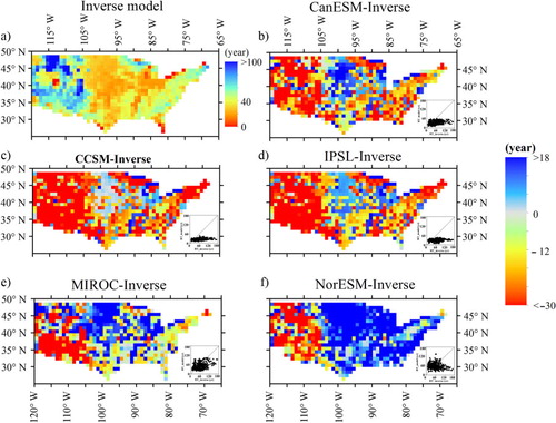
Table 3. Comparison NPP, NPP/GPP and mean residence time (MRT) in the USA and Australia between model-based and publication-based

	NPP (kg C m^−2 yr^−1)
Model	1850–1860	1995–2005	NPP/GPP	MRT cor (year) (USA)	MRT cor (year) (Australia)	Reference
CanESM	0.37	0.42	0.53	34	26
CCSM	0.31	0.34	0.42	24	18
IPSL	0.47	0.54	0.52	29	9
MIROC	0.45	0.49	0.52	49	30
NorESM1	0.17	0.18	0.18	55	40
Inverse model				46	Zhou and Luo (2008)**
Inverse model				56.8±8.8	Zhou et al. (2012)
VAST1.1 with genetic algorithm					78	Barret (2002)**
MODIS-based	0.475 (±0.375) (2000–2005)					Zhao and Running (2010)
MODIS-based	0.55 (2000–2003)		0.5 (2000–2003)			Zhang et al. (2009)

**MRT of Zhou and Luo (2008) and Barrett (2002) was estimated with NPP, so as comparison, MRT is corrected by the NPP/GPP ratio in the USA and in Australia.

4. Discussion

For ESMs, the ability to accurately represent the spatial distribution of NPP and MRT is a prerequisite for predicting ecosystem C storage capacity and future carbon–climate feedback. Our results showed that most models accurately predicted the global average NPP and NPP/GPP ratios compared with the MODIS estimates, although regional variability was relatively large among models (Table 3). However, all five models at the regional and global scales poorly estimated MRTs, resulting in poor estimates of ecosystem C storage capacity. Thus, variations in ecosystem C storage, NPP and MRT are important to improve model predictions of the global terrestrial C balance.

4.1. Variation in simulated ecosystem carbon storage capacity

Ecosystem C storage capacity can be a function of NPP and MRT and is composed of vegetation, litter and soil C pools. Currently, there is no feasible method to directly validate ecosystem C storage capacity due to the lack of the gridded observation-based data. Therefore, we indirectly assessed ecosystem C storage capacity through soil C storage and through validation of NPP and MRT. On average, none of the models accurately simulated the grid-scale distributions of ecosystem C storage capacity (Fig. 1) or soil C stocks, which were consistent with the results in Todd-Brown et al. (2013). Models may continue to amplify variation in predicting climate C-cycle feedback in the future (i.e. Friedlingstein et al., 2006).

It is evident that large variations remain in modelled estimates of ecosystem C storage capacity at the regional and global scales, with a high CV in most areas, particularly at high latitudes and in sparsely vegetated regions (Figs. 1 and 9). Large variation in ecosystem C storage capacity can result from high spatial variability in the NPP, MRT or both (Figs. 4 and 6). At 10° S–10° N, low variability in both the NPP and MRT resulted in little difference in ecosystem C storage capacity among models. At high latitudes and in sparsely vegetated regions, high CVs in NPP and MRT led to large variability in ecosystem C storage capacity. However, at lower latitudes, low variability in NPP and high variability of MRT also produced a high CV for ecosystem C storage capacity. In addition, the high spatial variability of NPP and MRT among individual models may induce large variability in C storage capacity. For example, if NorESM were not included, the CV for ecosystem C storage capacity would decrease by 27% on average, particularly at high latitudes. Our results suggest that the main source of variation in ecosystem C storage is spatial variability in C residence times, which was consistent with previous research at a regional scale (Zhou and Luo, 2008; Zhou et al., 2012). The inverse analysis indicated that the sensitivity of the C storage capacity to disturbance is determined by the residence time of C pool (Weng et al., 2012). Similarly, the results of Todd-Brown et al. (2013) showed indirectly that soil C turnover time was more important than NPP in determining differences of simulated soil C across ESMs at a global scale.

Another source of multi-model variation in ecosystem C storage capacity is likely the use of different methods to simulate the ecosystem C cycle. Most models are only effective for the specific processes in which they have been designed and their parameter ranges were validated (Dungait et al., 2012). For example, the soil models currently embedded in the ESMs are structured around 3–5 pools, with transformation rates modified by empirical correlations with soil temperature, water and clay content (Schmidt et al., 2011). However, mechanisms of permafrost melting over the long term are not embedded in the current ESMs, resulting in large uncertainties in prediction of ecosystem C storage at the steady state. Additionally, most ESMs ignored deep mineral soils or sparsely vegetated regions because of the lack of field data and ecosystem biogeochemistry. These omissions contribute to the large variation in ecosystem C storage at high latitudes and for Australia. For example, the current ESMs simulated C processes with 9–13 PFTs comprising forests and grasses, which largely omitted the property of permafrost vegetation. Models for permafrost soil C have only recently been integrated into ESMs (Koven et al., 2011) and further improvements in modelling C loss and accumulation would reduce uncertainties related to ecosystem C feedback cycles at high latitudes (Krishan et al., 2009; Schuur et al., 2009).

4.2. Variation in NPP and NPP/GPP ratio

Although most models reasonably predicted global NPP that was fairly consistent with latitude pattern (Fig. 7), none were able to reproduce grid-scale distributions of NPP (Fig. 9). Better performance at the latitude level may be due to aggregation of environmental variations that affect the C cycle at the grid scale. At the grid scale, land surface parameters may be the main factors contributing to poor agreement between the model predictions and empirical data. Most of the models share a similar structure in which photosynthetically fixed C is based on a leaf-level function. In the most models, PFT patches are directly linked to leaf-level ecophysiological measurements, while community composition (i.e. the PFTs and their areal extent) and vegetation structure (e.g. height, LAI) are directly inputted to each grid cell for each PFT. Thus, different inputs of land surface parameters among the models may cause spatial heterogeneity across models. For example, the land surface parameters in CLM were developed from several MODIS land surface products at a grid cell resolution of 0.05° (Lawrence and Chase, 2007), resulting in a good agreement between the simulated NPP for CCSM4 and NorESM with the estimated NPP from MODIS (Pearson correlation coefficient >0.7). In addition, the fixed vegetation cover in most ESMs would neglect the effect of climate change on vegetation. Among the five models, only MIROC models include dynamic vegetation through PFT distributional shifts and demographic stand process (Watanabe et al., 2011), which could directly produce the variability of vegetation cover over time and predict the C-climate feedback.

Fig. 9 Spatial pattern of coefficient of variation (CV) and standard deviation (SD) of NPP and MRT for all five models (modelled time: 1850–1860).

Although NPP is calculated from GPP and autotrophic respiration (R_a)_, little is known about the R_a and its response to environmental change, especially for long-term acclimation, which largely determine the NPP/GPP ratio. Plant R_a is not parameterised very well in current biogeochemical models (Atkin et al., 2008), further limiting the ability to accurately estimate NPP and its response to climate change. In most models, the sensitivity of R_a to temperature is represented by a Q₁₀ function or a modified Arrhenius equation (similar function), but different models have different Q₁₀ (Ruimy et al., 1996), ranging from 1.9 to 2.5 based on estimates inferred from global forest database (Piao et al., 2010). Moreover, the long-term experiments suggested that the sensitivity of plant respiration to temperature often declined with temperature due to the long-term acclimation (Luo, 2007; Atkin et al., 2008). Most ESMs defined a single temperature response function and failed to take into account for acclimation of plant respiration (Atkin et al., 2008).

4.3. Variation in MRT

In contrast to NPP, information on how ecosystem MRT varies among ecosystems and its responses to global climate change is extremely limited. Current research showed that soil warming experiments were compatible with the long-term sensitivity of SOC residence time (Knorr et al., 2005), with the slow soil C pool being more sensitive to temperature than the fast soil C pool, but it is still a topic of intense debate (Hopkins et al., 2012). Since future changes in the MRT could strongly affect the ability of the ecosystem to serve as a sink for atmospheric C, it is critical to evaluate model performance in estimating MRT against observed data. There are a number of factors that may contribute to poor agreement between model predictions and empirical data, such as variation in the observed data and model structure.

MRTs for various C pools are mainly estimated from simple isotope mixing models. Model estimates can only produce a composite MRT of the various SOC constituents with short and long residence times (Randerson et al., 1999), so different fractionation techniques and model structures may affect the calculation of MRT (Derrien and Amelung, 2011). As a result, global MRTs ranged from 29 to 60 yr (Table 2), which clearly indicates that there is room to improve the empirical estimates. Inverse models could be a valid approach to produce spatial information on MRTs at a global scale for assessing model performance. Although parameterisation of inverse models is constrained by experimental data, there have been large uncertainties reported, likely due to lack of experimental data (e.g. microbial biomass, respiration), a mismatch in timescales between the available data and the parameters to be estimated, or differences in the inverse methods (Xu et al., 2006; Zhou & Luo, 2008; Zhou et al., 2012). For example, the MRT estimated by Zhou and Luo (2008) was 10 yr shorter than the estimate by Zhou et al. (2012) using different inverse methods with nearly the same experimental data.

Improving empirical estimates, however, will not fully resolve the differences in MRT predictions across models, because they do not all agree with one another in their representation of the ecosystem. MRTs are estimated from C transfer coefficients among the various C pools and environmental forcing (Xia et al., 2013). The former determines how long C may remain in plant or soil pool. The C allocated to plant tissues (e.g. stems, leaves and roots) could determine ecosystem MRT, commonly described by plant biomass or PFTs (Carbone and Trumbore, 2007). For example, the low allocation of C to the longer-lived stem pools resulted in the short MRT for biomass C in Arid region (Barrett, 2002). The cropland and grassland only allocate C to leaves and roots with turnover times of months to a few years, leading to the lower MRT than other PFTs (Zhou et al., 2012). However, among five models, only MIROC simulates the temporal dynamics of PFTs. Another source of the large variation is to determine C transfer coefficients between pools. For example, in the MIROC models, the transfer coefficients from the leaves and fine roots into the litter are constant (Sato et al., 2007), while in the CanESM models, they are calculated as a function of normal turnover, drought and cold stress (Arora and Boer, 2005). Highly variable C residence times in difference pools would lead to the difference of ecosystem MRT among models globally and regionally. For example, grassland and cropland have the relatively fast MRT due to the lack of long-residence wood tissues and coarse litter (Zhou et al., 2012).

The difference of MRT across models could result from ecosystem response to driving variables, determined by model parameterisation. Here, we defined MRT as a function of soil temperature (T_s): , where the parameter k and Q₁₀ in each model were calculated using ecosystem MRT and climate factors across all grid cells. Such simple models showed that temperature could explain the spatial variation of ecosystem MRT up to 65% (Table 4), suggesting the effects of the initial residence time and the temperature sensitivity on ecosystem MRT among models. The Q₁₀ values in MIROC, CanESM and IPSL were within the range between 1.5 and 2.5, which have been often set on estimates inferred from ecosystem flux measurements (Mahecha et al., 2010), while Q₁₀ in CCSM and NorESM was much higher, resulting in the short MRT. In addition, soil moisture did not significantly improve the estimate of MRT if it was incorporated into the temperature function (data not shown).

Table 4. Q₁₀ variance across models (function: )

Model	k (yr)	Q 10	R ^2
CanESM	19.4	1.83	0.61
CCSM	3.5	3.89	0.65
IPSL	13.7	1.43	0.59
MIROC	36.6	1.52	0.58
NorESM1	2.4	5.06	0.63

4.4. Implications for land surface models

Our model intercomparison indicates that both NPP and MRT may contribute to multi-model variation in ecosystem C storage capacity at the regional scale but MRT has greater effects than NPP, especially at high latitudes. More research on carbon MRT is thus needed to greatly improve the performance of land surface models toward predictive understanding of ecosystem responses to climate change in the future. Thus, our study would offer several suggestions for future experimental and modelling research with the goal of improving estimates of ecosystem C storage capacity.

First, our results showed that some ESMs such as CCSM4 simulated fast C turnover, whereas other models such as MIROC simulated slow C turnover (Fig. 6). Thus, experimental data of C residence time in various C pools should be used to constrain the rates of the C cycle. In addition, there are no benchmarking data for the spatial patterns of MRT at regional or global scale to assess model performance. Inverse models would be a reasonable approach to produce a map of ecosystem MRTs. Thus, collection of experimental data on various C pools among biomes globally is the first step to improve model parameters. Especially, models could use forest inventory data to constrain C residence times in living biomass pools.

Second, although most models share a similar structure for carbon partitioning among three or more C pools and response to climate change, the models have different definitions of the C pools and equations with environmental variables that control the C flows among the C pools, resulting in large variation in simulation of ecosystem MRT. For example, IPSL defines 15 C pools (eight biomass pools, four litter pools and three soil C pools), while CLM4 simulates six C pools (three biomass pools and three dead C pools). Thus, assessing and improving C partitioning and transfer coefficients among C pools at the global scale is key to improving model performance for ecosystem MRTs.

Third, this study demonstrated that the largest uncertainties in spatial variability of ecosystem C storage and MRTs occur at high latitudes and for sparsely vegetated regions (Figs. 1 and 6). The current soil models embedded in ESMs are mainly based on molecular structures and the kinetic theory (Schmidt et al., 2011). Such model structures largely ignore deep mineral and permafrost soils. In addition, there would be a strong temperature or water stress close to thresholds for vegetation growth in the sparse vegetated regions, which could be difficult to be modelled accurately. Thus, it is imperative for the development of ESMs to improve post-photosynthesis C cycle modelling at high latitudes and its response to climate change.

5. Conclusions

We aimed to evaluate spatial variation in ecosystem C storage capacity simulated by ESMs included in CMIP5 and to examine sources of multi-model variability in the results associated with MRT and/or C inputs. Model intercomparison indicated that NPP was simulated relatively well by most models on average, but MRT was substantially underestimated by most of the models. Underestimation of MRT resulted in lower estimates for ecosystem C storage capacity. Among the five models, MIROC predicted the largest ecosystem C storage capacity (about 40 kg C m⁻²) and the longest MRT (50 yr). The spatial patterns of ecosystem C storage capacity predicted by CCSM4 and NorESM were similar, as they include the same land C model (e.g. CLM). The C storage capacity estimated by NorESM was higher than that for CCSM due to differences in the NPP/GPP ratio between the two models. Nonetheless, large spatial variations in MRT and NPP resulted in large variations in ecosystem C storage capacity (CV=0.4–1.2), particularly at high latitudes and in sparsely vegetated regions. Our results indicate that more research should be conducted in the future to estimate C partitioning and transfer coefficients among C pools so that ecosystem C residence time and storage capacity can be accurately simulated.

6. Acknowledgements

This study was funded by the Program for Professor of Special Appointment (Eastern Scholar) at Shanghai Institutions of Higher Learning, 2012 Shanghai Pujiang Program (12PJ1401400), Thousand Young Talents Program in China, by a Changjiang Scholarship to Yiqi Luo at Fudan University, and by the US Department of Energy Terrestrial Ecosystem Sciences Grant DE SC0008270 and US National Science Foundation (NSF) Grants DEB 0444518, DEB 0743778, DEB 0840964, DBI 0850290 and EPS 0919466 to YL at the University of Oklahoma. We acknowledge the World Climate Research Programmer's Working Group on Coupled Modelling, which is responsible for CMIP, and we thank the climate modelling groups (Table 1) for producing and making available their model output. Additional thanks to CMIP, the US Department of Energy's Program for Climate Model Diagnosis and Intercomparison, for providing coordinating support and leading the development of software infrastructure in partnership with the Global Organization for Earth System Science Portals.

References

- Ahlström A , Smith B , Lindström J , Rummukainen M , Uvo C. B . GCM characteristics explain the majority of uncertainty in projected 21st century terrestrial ecosystem carbon balance. Biogeosciences. 2013; 10: 1517–1528.
- Arora V. K , Boer G. J . A parameterization of leaf phenology for the terrestrial ecosystem component of climate models. Glob. Chang. Biol. 2005; 11: 39–59.
- Arora V. K , Scinocca J. F , Boer G. J , Christian J. R , Denman K. L , co-authors . Carbon emission limits required to satisfy future representative concentration pathways of greenhouse gases. Geophys. Res. Lett. 2011; 38: 05805.
- Atkin O. K , Atkinson L. J , Fisher R. A , Campbell C. D , Zaragoza-Castells J , co-authors . Using temperature-dependent changes in leaf scaling relationships to quantitatively account for thermal acclimation of respiration in a coupled global climate–vegetation model. Glob. Chang. Biol. 2008; 14: 2709–2726.
- Barrett D. J . Steady state turnover time of carbon in the Australian terrestrial biosphere. Glob. Biogeochem. Cycles. 2002; 16(4): 1108.
- Bowman D. M, Balch J. K, Artaxo P, Bond W. J, Carlson J. M, co-authors. Fire in the Earth system. Science. 2009; 324: 481–484. [PubMed Abstract].
- Canadell J. G, Le Quere C, Raupach M. R, Field C. B, Buitenhuis E. T, co-authors. Contributions to accelerating atmospheric CO2 growth from economic activity, carbon intensity, and efficiency of natural sinks. Proc. Natl. Acad. Sci. U. S. A. 2007; 104: 18866–18870. [PubMed Abstract] [PubMed CentralFull Text].
- Carbone M. S, Trumbore S. E. Contribution of new photosynthetic assimilates to respiration by perennial grasses and shrubs: residence times and allocation patterns. New Phytol. 2007; 176: 124–135. [PubMed Abstract].
- Chambers J. Q, Fisher J. I, Zeng H, Chapman E. L, Baker D. B, co-authors. Hurricane Katrina's carbon footprint on U.S. Gulf Coast forests. Science. 2007; 318: 1107. [PubMed Abstract].
- Ciais P , Friedlingstein P , Schimel D. S , Tans P. P . A global calculation of the delta C-13 of soil respired carbon: implications for the biospheric uptake of anthropogenic CO2 . Glob. Biogeochem. Cycles. 1999; 13: 519–530.
- Cox P. M , Betts R. A , Collins M , Harris P. P , Huntingford C , co-authors . Amazonian forest dieback under climate–carbon cycle projections for the 21st century. Theor. Appl. Climatol. 2004; 78: 137–156.
- Cramer W , Field C. B . Comparing global models of terrestrial net primary productivity (NPP): introduction. Glob. Chang. Biol. 1999; 5: Iii–Iv.
- Cramer W , Kicklighter D. W , Bondeau A , Moore B , Churkina G , co-authors . Comparing global models of terrestrial net primary productivity (NPP): overview and key results. Glob. Chang. Biol. 1999; 5: 1–15.
- Davidson E. A, Janssens I. A. Temperature sensitivity of soil carbon decomposition and feedbacks to climate change. Nature. 2006; 440: 165–173. [PubMed Abstract].
- Derrien D , Amelung W . Computing the mean residence time of soil carbon fractions using stable isotopes: impacts of the model framework. Eur. J. Soil Sci. 2011; 62: 237–252.
- Dungait J. A. J , Hopkins D. W , Gregory A. S , Whitmore A. P . Soil organic matter turnover is governed by accessibility not recalcitrance. Glob. Chang. Biol. 2012; 18: 1781–1796.
- Emanuel W. R , Killough G. G , Post W. M , Shugart H. H . Modeling terrestrial ecosystems in the global carbon-cycle with shifts in carbon storage capacity by land-use change. Ecology. 1984; 65: 970–983.
- FAO/IIASA/ISRIC/ISSCAS/JRC. Harmonized World Soil Database (version 1.10). 2012; Rome, Italy and IIASA, Laxenburg, Austria: FAO.
- Friedlingstein P , Cox P , Betts R , Bopp L , Von Bloh W , co-authors . Climate–carbon cycle feedback analysis: results from the C4MIP model intercomparison. J. Clim. 2006; 19: 3337–3353.
- Heimann M, Reichstein M. Terrestrial ecosystem carbon dynamics and climate feedbacks. Nature. 2008; 451: 289–292. [PubMed Abstract].
- Hiederer R , Köchy M . Global Soil Organic Carbon Estimates and the Harmonized World Soil Database. EUR 25225 EN. 2011; Publications Office of the European Union. 79 pp.
- Hopkins F. M, Torn M. S, Trumbore S. E. Warming accelerates decomposition of decades-old carbon in forest soils. Proc. Natl. Acad. Sci. U. S. A. 2012; 109: E1753–1761. [PubMed Abstract] [PubMed CentralFull Text].
- Johnston M. H , Homann P. S , Engstrom J. K , Grigal D. F . Changes in ecosystem carbon storage over 40 years on an old-field forest landscape in east-central Minnesota. Forest Ecol. Manag. 1996; 83: 17–26.
- Kane E. S , Vogel J. G . Patterns of total ecosystem carbon storage with changes in soil temperature in Boreal Black Spruce forests. Ecosystems. 2009; 12: 322–335.
- Kicklighter D. W , Bondeau A , Schloss A. L , Kaduk J , McGuire A. D , co-authors . Comparing global models of terrestrial net primary productivity (NPP): global pattern and differentiation by major biomes. Glob. Chang. Biol. 1999; 5: 16–24.
- Knorr W, Prentice I. C, House J. I, Holland E. A. Long-term sensitivity of soil carbon turnover to warming. Nature. 2005; 433: 298–301. [PubMed Abstract].
- Koven C. D, Ringeval B, Friedlingstein P, Ciais P, Cadule P, co-authors. Permafrost carbon–climate feedbacks accelerate global warming. Proc. Natl. Acad. Sci. U. S. A. 2011; 108: 14769–14774. [PubMed Abstract] [PubMed CentralFull Text].
- Krinner G , Viovy N , de Noblet-Ducoudré N , Ogée J , Polcher J , co-authors . A dynamic global vegetation model for studies of the coupled atmosphere-biosphere system. Glob. Biogeochem. Cycles. 2005; 19: GB1015.
- Krishan G , Srivastav S. K , Kumar S , Saha S. K , Dadhwal V. K . Quantifying the underestimation of soil organic carbon by the Walkley and Black—examples from Himalayan and Central Indian soils. Curr. Sci. India. 2009; 96: 1133–1136.
- Lales J. S , Lasco R. D , Geronimo I. Q . Carbon storage capacity of agricultural and grassland ecosystems in a geothermal block. Philippine Agr. Sci. 2001; 84: 8–18.
- Lawrence D. M , Oleson K. W , Flanner M. G , Thornton P. E , Swenson S. C , co-authors . Parameterization improvements and functional and structural advances in version 4 of the Community Land Model. J. Adv. Model. Earth Syst. 2011; 3: 1942–2466.
- Lawrence P. J , Chase T. N . Representing a new MODIS consistent land surface in the Community Land Model (CLM 3.0). Journal of Geophysical Research: Biogeosciences. 2007; 112: G01023.
- Le Quere C , Raupach M. R , Canadell J. G , Marland G , Bopp L , co-authors . Trends in the sources and sinks of carbon dioxide. Nat. Geosci. 2009; 2: 831–836.
- Luo Y . Terrestrial carbon–cycle feedback to climate warming. Ann. Rev. Ecol. Evol. Syst. 2007; 38: 683–712.
- Luo Y. Q , White L. W , Canadell J. G , DeLucia E. H , Ellsworth D. S , co-authors . Sustainability of terrestrial carbon sequestration: a case study in Duke Forest with inversion approach. Glob. Biogeochem. Cycles. 2003; 17(1): 1021.
- Luo Y. Q , Wu L. H , Andrews J. A , White L , Matamala R , co-authors . Elevated CO2 differentiates ecosystem carbon processes: deconvolution analysis of Duke Forest FACE data. Ecol. Monogr. 2001; 71: 357–376.
- Mahecha M. D, Reichstein M, Carvalhais N, Lasslop G, Lange H, co-authors. Global convergence in the temperature sensitivity of respiration at ecosystem level. Science. 2010; 329: 838–840. [PubMed Abstract].
- Meyer R , Joos F , Esser G , Heimann M , Hooss G , co-authors . The substitution of high-resolution terrestrial biosphere models and carbon sequestration in response to changing CO2 and climate. Global Biogeochem. Cycles. 1999; 13: 785–802.
- Mooney H , Canadell J , Chapin F., III , Ehleringer J , Körner C , co-authors . Ecosystem Physiology Responses to Global Change. 1999; Cambridge: Cambridge University Press. 141–189.
- Parton W. J , Stewart J. W , Cole C. V . Dynamics of C, N, P and S in grassland soils: a model. Biogeochemistry. 1988; 5: 109–131.
- Piao S, Luyssaert S, Ciais P, Janssens I. A, Chen A, co-authors. Forest annual carbon cost: a global-scale analysis of autotrophic respiration. Ecology. 2010; 91: 652–661. [PubMed Abstract].
- Pinsonneault A. J , Matthews H. D , Kothavala Z . Benchmarking climate–carbon model simulations against forest FACE data. Atmos. Ocean. 2011; 49: 41–50.
- Prentice I. C , Bondeau A , Cramer W , Harrison S. P , Hickler T , co-authors . Dynamic global vegetation modeling: quantifying terrestrial ecosystem responses to large-scale environmental change. Terrestrial Ecosystems in a Changing World. 2007; Springer, Berlin,: Heidelberg. 175–192. (eds. J. G. Canadell, D. E. Pataki and L..
- Raich J. W , Schlesinger W. H . The global carbondioxide flux in soil respiration and its relationship to vegetation and climate. Tellus B. 1992; 44: 81–99.
- Randerson J. T , Thompson M. V , Field C. B . Linking C-13-based estimates of land and ocean sinks with predictions of carbon storage from CO2 fertilization of plant growth. Tellus. B. 1999; 51: 668–678.
- Ruimy A , Dedieu G , Saugier B . TURC: a diagnostic model of continental gross primary productivity and net primary productivity. Glob. Biogeochem. Cycles. 1996; 10: 269–285.
- Sato H , Itoh A , Kohyama T . SEIB–DGVM: a new dynamic global vegetation model using a spatially explicit individual-based approach. Ecol. Model. 2007; 200: 279–307.
- Schmidt M. W. I, Torn M. S, Abiven S, Dittmar T, Guggenberger G, co-authors. Persistence of soil organic matter as an ecosystem property. Nature. 2011; 478: 49–56. [PubMed Abstract].
- Schuur E. A. G, Vogel J. G, Crummer K. G, Lee H, Sickman J. O, co-authors. The effect of permafrost thaw on old carbon release and net carbon exchange from tundra. Nature. 2009; 459: 556–559. [PubMed Abstract].
- Solomon S , Qin D , Manning M , Marquis M , Averyt K , co-authors . Climate change 2007: the physical science basis. Contribution of Working Group I to the Fourth Assessment Report of the Intergovernmental Panel on Climate Change. 2007; Cambridge: Cambridge University Press.
- Strassmann K. M , Joos F , Fischer G . Simulating effects of land use changes on carbon fluxes: past contributions to atmospheric CO2 increases and future commitments due to losses of terrestrial sink capacity. Tellus B. 2008; 60: 583–603.
- Tang J. W , Yin J. X , Qi J. F , Jepsen M. R , Lu X. T . Ecosystem carbon storage of tropical forests over limestone in Xishuangbanna, SW China. J. Trop. Forest Sci. 2012; 24: 399–407.
- Thompson M. V , Randerson J. T . Impulse response functions of terrestrial carbon cycle models: method and application. Glob. Chang. Biol. 1999; 5: 371–394.
- Tian H. Q , Chen G. S , Zhang C , Liu M. L , Sun G , co-authors . Century-scale responses of ecosystem carbon storage and flux to multiple environmental changes in the southern united states. Ecosystems. 2012; 15: 674–694.
- Todd-Brown K. E. O , Randerson J. T , Post W. M , Hoffman F. M , Tarnocai C , co-authors . Causes of variation in soil carbon simulations from CMIP5 Earth system models and comparison with observations. Biogeosciences. 2013; 10: 1717–1736.
- van der Werf G. R , Randerson J. T , Giglio L , Collatz G , Mu M , co-authors . Global fire emissions and the contribution of deforestation, savanna, forest, agricultural, and peat fires (1997–2009). Atmos. Chem. Phys. 2010; 10: 11707–11735.
- Wang W , Dungan J , Hashimoto H , Michaelis A. R , Milesi C , co-authors . Diagnosing and assessing uncertainties of terrestrial ecosystem models in a multimodel ensemble experiment: 1. primary production. Glob. Chang. Biol. 2011; 17: 1350–1366.
- Weng E. S , Luo Y. Q , Wang W , Wang H , Hayes D. J , co-authors . Ecosystem carbon storage capacity as affected by disturbance regimes: A general theoretical model. Journal of Geophysical Research-Biogeosciences. 2012; 117: G3.
- Watanabe S , Hajima T , Sudo K , Nagashima T , Takemura T , co-authors . MIROC-ESM 2010: model description and basic results of CMIP5-20c3m experiments. Geosci. Model Dev. 2011; 4: 845–872.
- Xia J, Luo Y, Wang Y. P, Hararuk O. Traceable components of terrestrial carbon storage capacity in biogeochemical models. Glob. Chang. Biol. 2013; 19: 2104–2116. [PubMed Abstract].
- Xu T , White L , Hui D. F , Luo Y. Q . Probabilistic inversion of a terrestrial ecosystem model: analysis of uncertainty in parameter estimation and model prediction. Glob. Biogeochem. Cycles. 2006; 20: GB2007.
- Zhang Y , Xu M , Chen H , Adams J . Global pattern of NPP to GPP ratio derived from MODIS data: effects of ecosystem type, geographical location and climate. Glob. Ecol. Biogeogr. 2009; 18: 280–290.
- Zhao M, Running S. W. Drought-induced reduction in global terrestrial net primary production from 2000 through 2009. Science. 2010; 329: 940–943. [PubMed Abstract].
- Zhou T , Luo Y. Q . Spatial patterns of ecosystem carbon residence time and NPP-driven carbon uptake in the conterminous United States. Glob. Biogeochem. Cycles. 2008; 22: GB3032.
- Zhou X , Zhou T , Luo Y . Uncertainties in carbon residence time and NPP-driven carbon uptake in terrestrial ecosystems of the conterminous USA: a Bayesian approach. Tellus B. 2012; 64: 17223.