Effects of cooling and internal wave motions on gas transfer coefficients in a boreal lake

Abstract

Lakes and other inland waters contribute significantly to regional and global carbon budgets. Emissions from lakes are often computed as the product of a gas transfer coefficient, k ₆₀₀ , and the difference in concentration across the diffusive boundary layer at the air–water interface. Eddy covariance (EC) techniques are increasingly being used in lacustrine gas flux studies and tend to report higher values for derived k ₆₀₀ than other approaches. Using results from an EC study of a small, boreal lake, we modelled k ₆₀₀ using a boundary-layer approach that included wind shear and cooling. During stratification, fluxes estimated by EC occasionally were higher than those obtained by our models. The high fluxes co-occurred with winds strong enough to induce deflections of the thermocline. We attribute the higher measured fluxes to upwelling-induced spatial variability in surface concentrations of CO₂ within the EC footprint. We modelled the increased gas concentrations due to the upwelling and corrected our k ₆₀₀ values using these higher CO₂ concentrations. This approach led to greater congruence between measured and modelled k values during the stratified period. k ₆₀₀ has a well-resolved and ~cubic relationship with wind speed when the water column is unstratified and the dissolved gases well mixed. During stratification and using the corrected k ₆₀₀ , the same pattern is evident at higher winds, but k ₆₀₀ has a median value of ~7 cm h⁻¹ when winds are less than 6 m s⁻¹, similar to observations in recent oceanographic studies. Our models for k ₆₀₀ provide estimates of gas evasion at least 200% higher than earlier wind-based models. Our improved k ₆₀₀ estimates emphasize the need for integrating within lake physics into models of greenhouse gas evasion.

• carbon dioxide
• gas transfer
• upwelling
• eddy covariance
• heat flux
• thermocline tilting

1. Introduction

Lakes are disproportionately active sites in carbon cycling relative to their surface area (Cole et al., 2007), and with more accurate estimates of their numbers and surface area (Downing et al., 2006), emissions have been found to be significant relative to the terrestrial sources and sinks. The global estimate for the terrestrial uptake of CO₂ is 3.0±0.9 Pg C yr⁻¹ (Le Quéré et al., 2009), and the global evasion rate from lakes and reservoirs is now estimated at 0.32 Pg C yr⁻¹ (Raymond et al., 2013). Many of the initial efforts demonstrating the contribution of inland waters to greenhouse gas evasion were based on measurements of fluxes with chambers on the water surface, by tracer studies, or by computing fluxes as the product of a gas transfer coefficient times the concentration gradient across the diffusive boundary layer at the air–water interface (Kling et al., 1992; Richey et al., 2002). In much of the recent effort to place emissions from lakes into the context of regional carbon budgets, computations were done using either a conservative value of the gas transfer coefficient or one based on wind speed (Cole and Caraco, 1998). Use of eddy covariance (EC) has led to upward predictions of gas evasion (Jonsson et al., 2008) relative to Cole and Caraco (1998) with some studies indicating that fluxes are enhanced under heating (McGillis et al., 2004) and others with cooling (MacIntyre et al., 2010). Similarly, more comprehensive models of the gas transfer coefficient indicate that improved accuracy may result from including other terms besides wind when estimating fluxes (Soloviev and Schlüssel, 1994; Soloviev et al., 2007).

The relative contribution of wind and buoyancy flux to turbulence at the air–water interface varies with lake size (Read et al., 2012). As small lakes are orders of magnitude more abundant than large lakes (Downing et al., 2006), further evaluation of their hydrodynamics as it applies to gas flux is required. For example, in northern latitudes many lakes are small, and in Finland >95% of the 190 000 lakes have an area <1 km² and in total can cover locally up to 20% of the land area (Raatikainen and Kuusisto, 1990), and thus play an especially important role in regional carbon cycling. As turbulence mediates gas flux across the air–water interface (Zappa et al., 2007; MacIntyre et al., 2010; Vachon et al., 2010), the concern has been raised as to whether wind-speed-based parameterizations are applicable or need to be modified for small lakes (Read et al., 2012). By definition, at depths above the Monin-Obukhov length scale, L, which is the ratio of u _*w ³/0.4β, where u _*w is the aquatic friction velocity, 0.4 is the von Karman constant and β the buoyancy flux (Imberger, 1985), wind-induced shear dominates turbulence production, whereas at depths below it, convection dominates. If that scaling is correct, wind shear would always be the dominant driver of emissions. Further, if turbulence is the dominant control on evasion at the air–water interface, a cubic dependency on wind speed is expected (Wanninkhof et al., 2009). Thus, with their numerical abundance in the landscape, understanding operative processes at the air–water interface in small lakes requires studies which quantify wind shear and buoyancy flux, and determines the relative contribution of each to the gas transfer coefficient.

Wind and cooling moderate gas transfer to the air–water interface. Their relative contribution has not been addressed for small lakes. The effect of wind on different strata can be predicted from the Wedderburn number, W, or its integral form, the Lake number, L _N , which indicates the degree of thermocline tilting as a function of wind speed, the density gradient across the thermocline and basin morphometry (Imberger and Patterson, 1990). For high values of W, wind will only stir near surface waters. As W decreases below about 10, the thermocline begins to tilt. For W<3, mixing is anticipated near the margins; for W≤1, full upwelling is predicted plus considerable mixing throughout the thermocline and into the mixed layer (Monismith, 1985; MacIntyre et al., 1999; Horn et al., 2001; Boegman et al., 2005). The thermals produced during convection penetrate throughout the mixed layer and can cause entrainment of waters with higher concentrations of dissolved gases to the air–water interface (Crill et al., 1988; Eugster et al., 2003). Time series studies in small arctic lakes, with their reduced density difference across the thermocline, demonstrate that thermocline tilting and exchange between the upper mixed layer and more stratified layers can occur frequently, and mixed layer deepening and entrainment by convection are likely during cloudy conditions (MacIntyre et al., 2009). For boreal lakes, the density gradient across the thermocline will be larger in summer, but during fall cooling as it decreases, internal wave motions and convection could both contribute in bringing dissolved gases to the air–water interface and thus mediate increased fluxes.

EC systems, with their direct continuous measurements of flux (F), enable improved estimates of gas transfer coefficient, k (Eugster et al., 2003; Nordbo et al., 2011; Vesala et al., 2012). Using inverse procedures, the gas transfer coefficient k is computed as k=F/(c _aq −c _eq ), where c _aq is concentration of the dissolved gas in water and c _eq is the concentration in the water in equilibrium with the atmosphere. The gas transfer coefficient is generally normalized to CO₂ at 20°C and called k ₆₀₀ . For the inverse procedure to be accurate in lakes, the footprint of the system must not reach onto the surrounding land (Eugster et al., 2003; Vesala et al., 2006), and the measurement of water concentration must be representative of the full footprint. In most cases, dissolved gases are only obtained at one location, although there are a number of studies which illustrate the spatial variability of dissolved gases (Roland et al., 2010; Rudorff et al., 2011; Abril et al., 2013). Spatial variability is expected if wind induces tilting of the thermocline, and some gases are mixed into the mixed layer either with the initial wind forcing or when the thermocline rebounds on cessation of the wind. Spatial variability would also result if the mixing from nocturnal cooling, which brings dissolved gases to the air–water interface (Crill et al., 1988), penetrated to different depths as would be expected if some parts of a lake basin were more exposed to wind and with concomitant higher evaporation rates. Lastly, processes such as differential cooling would bring gases produced nearshore to offshore sites where they could be mixed vertically by convection. Hence, evaluation of the accuracy of estimates of k ₆₀₀ from EC systems must consider whether spatial heterogeneity in gas concentrations has confounded the estimates.

Here we present results of a study using EC to quantify evasion of CO₂ and the gas transfer coefficient in a small boreal lake during fall cooling. We developed an equation for the gas transfer coefficient based on boundary-layer theory, which took into account both wind speed and buoyancy flux. This equation is independent of the empiricism inherent in applications of the surface renewal model which currently rely on similarity scaling from ocean sites for estimates of turbulence (MacIntyre et al., 2001, 2010; Eugster et al., 2003; Read et al., 2012). We evaluated the new model and k from the surface renewal model and from regression equations in MacIntyre et al. (2010) relative to k from the EC system. With this approach, and computation of the Wedderburn and Lake numbers plus cooling, we were able to evaluate the accuracy of our modelling and assess whether gas concentrations were sometimes higher in the EC footprint due to quantifiable within lake motions. We evaluate the measured k ₆₀₀ during different conditions and compare it to the wind-based equation (Cole and Caraco, 1998) used in regional carbon budgets. With these combined approaches, we assess the physical processes which need to be included in modelling greenhouse gas evasion in small lakes.

2. Site and methods

2.1. Field site

The fieldwork was carried out in Finland in the humic Lake Kuivajärvi (61°50′ N, 24°17′ E) in Hyytiälä [Station for Measuring Forest Ecosystem–Atmosphere Relations (SMEAR) II]. The site is part of the ICOS (Integrated Carbon Observation System) measuring network, and the carbon and energy exchange between the forest and atmosphere at the site has been intensively studied (e.g. Kolari et al., 2009; Launiainen, 2010). The lake has an area of 63.8 ha and a catchment area dominated by a managed Scots pine (Pinus sylvestris L.) forest. Lake Kuivajärvi is a long and narrow north–south-oriented lake (Fig. 1), and with two distinct basins. The deeper south basin reaches a maximum depth of 13.2 m, making Kuivajärvi deeper than most lakes in Finland, since the mean value of the maximum depths of Finnish lakes is 8.2 m (Kortelainen et al., 2006). Lake Kuivajärvi is in the upper part of the Kokemäenjoki River basin, which drains to the Bothnian Sea in the northern part of the Baltic Sea.

Fig. 1 Contour map and wind rose for Lake Kuivajärvi. The location of the platform is indicated with the white cross. The wind directions in degrees are on the circumference and the lengths of the blue arrows indicate the wind speeds (m s⁻¹).

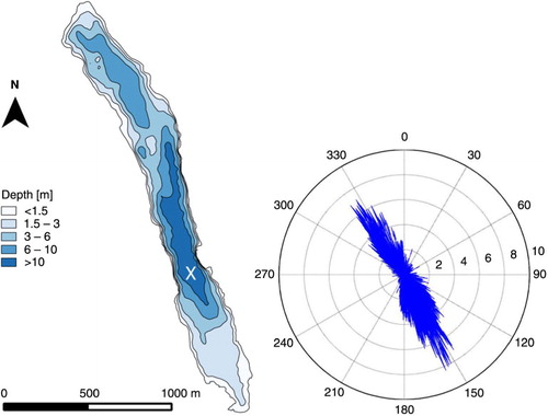
The measurements were taken on a platform situated in the middle of the lake. The fetch is longest at the platform when the wind blows from 320° to 350°, approximately 1.8 km, or from 130° to 180°, approximately 0.8 km. From other directions, the fetch is only 0.4 km at maximum.

2.2. Measurements

The measurements were carried out from 9 August to 30 November 2011; that is, they covered the end of the summer stratification period as well as the period of autumn overturn.

The EC measuring system on the platform was comprised of a Metek ultrasonic anemometer (USA-1; Metek GmbH, Elmshorn, Germany), which measured the three wind speed components and an enclosed path infrared gas analyzer LI-7200 (Li-Cor, Inc., Lincoln, NE, USA). The measuring height, z _m , was 1.5 m above the water surface. The length of the polytetrafluoroethylene (PTFE) sampling tube was 1.8 m and the inner diameter was 8 mm. The flow rate was 12 L min⁻¹, providing a turbulent flow. The tube was heated (3 W m⁻¹) to avoid condensation. Sampling frequency was 10 Hz. The micrometeorological fluxes were calculated following Mammarella et al. (2009) and Aubinet et al. (2012). Several quality-screening criteria were applied to the EC data, including the flux stationarity test (Foken and Wichura, 1996), limits for skewness and kurtosis of scalar quantities and vertical wind velocity, as well as visual inspection of power spectra and cospectra. Much of the data during light winds and cooling did not pass the stationarity tests, z _m /L>−0.55, and was not considered in the analysis. Therefore, most of the nightly data early in the period were missing. EC data post-processing and adopted quality criteria follow those used in Vesala et al. (2006) and Nordbo et al. (2011).

We obtained continuous measurements of water column concentrations of CO₂ at depths of 0.2, 0.5, 1.0 and 3.0 m by using a similar measuring system as Hari et al. (2008), in which a continuous airstream was circulated with a diaphragm pump (KNF Neuberger Micro gas pump; KNF Neuberger AB, Stockholm, Sweden) in a closed loop. The system consisted of gas-impermeable tubing (stainless steel and Teflon), a CO₂ analyzer (CARBOCAP® GMP343; Vaisala Oyj, Vantaa, Finland), semipermeable silicone rubber tubing with 1.5-mm wall thickness (Rotilabo 9572.1; Carl Roth GmbH & Co. KG, Karlsruhe, Germany) for gas collection and the pump. The semipermeable tubing was placed at the respective measuring depths. The gas collection tubing, CO₂ analyzer and pump were connected with gas-impermeable tubing. The gas concentrations in the continuous airstream within the loop equilibrated with those in water around the semipermeable tubing; thus, the CO₂ concentration in the water could be continuously measured in the gaseous phase. The silicone rubber was cleaned weekly during the open-water period by gently scrubbing the surface, and the rubber was entirely replaced every other month. The data were logged at 1-minute intervals. We additionally measured CO₂ profiles at weekly intervals using the head space method (López Bellido et al., 2009).

For water temperature measurements, a chain of Pt100 temperature sensors was installed with sensors at depths of 0.2, 0.5, 1.0, 1.5, 2.0, 2.5, 3.0, 3.5, 4.0, 4.5, 5.0, 6.0, 8.0 and 10 m to continuously record water temperature. The sensors were new and calibrated at the factory. The accuracy of the sensors is 0.2°C and the response time 15 second, the data was recorded at 0.1°C resolution, the logging interval 5 second and the values at 0.2 m were used to represent surface water temperatures in the calculations. The incoming and outgoing longwave and shortwave radiation was measured with a CNR-1 net radiometer (Kipp & Zonen B.V., Delft, The Netherlands).

2.3. The measured gas transfer velocity

The gas transfer velocity was calculated from measurements as:1

where is the EC CO₂ flux, c _aq is the surface water CO₂ concentration and c _eq is the equilibrium CO₂ concentration. Assuming that standard conditions prevail, the atmospheric pressure of CO₂ can be calculated as follows:2

where is the mole fraction of CO₂ (given by the EC), and p _atm is the atmospheric pressure (=1 atm). The equilibrium concentration of CO₂ (mol L⁻¹) in the surface water is calculated using Henry's law:3

where k _H is the Henry's law constant at the surface water temperature. For c _eq in g m⁻³, the results must be multiplied with the molar mass of CO_2, thus resulting in the following final equation for equilibrium concentration:4

The calculations for the bulk CO₂ concentrations in water, c _aq , were made as with the equilibrium concentration in eqs. (2) and (4), and the mole fraction of CO₂ was from the Vaisala probes. We used the data from the 0.2 m probe as the surface CO₂ concentration, but we also computed expected CO₂ concentration within the footprint taking into account the extent of thermocline deflection based on calculations of the Wedderburn and Lake numbers and our estimates of the depth of the actively mixing layer, and denote the gas transfer velocities obtained as k _site and k _fp , where site stands for measurement site and fp for footprint. The Wedderburn number is a dimensionless ratio of the density stratification to the wind forcing and aspect ratio of the lake (Monismith, 1986):5

where Δρ is the density difference between the epilimnion and the hypolimnion, ρ ₀ the mean density of the water column, g the acceleration due to gravity, h ₁ the depth of the epilimnion, L ₁ the length of the lake and u _*w the friction velocity in water. A related index is the Lake number (Imberger and Patterson, 1990):6

where S is the overall stability of the lake, z _t the height of the centre of the metalimnion, H the depth of the lake, A the lake area and z _g the height to the centre of the volume of the lake. L _N , similarly to W, captures the influence of stratification, wind stress, and basin morphometry, and we use the indices identically in the following (MacIntyre et al., 1999). For W of order 1, CO₂-rich metalimnetic waters would reach the surface. For partial upwelling with cooling either during or after the event, convection would mix water with higher CO₂ concentrations into the upper mixed layer. For this purpose, we derived an equation which predicts the depth, z _E , where E denotes for entrainment, at which the CO₂ might reach the surface:7

where h ₁ /W is the maximum thermocline displacement (Monismith, 1986; Horn et al., 2001) and z _AML the depth of the actively mixing layer. The z _AML has been defined operationally as the depth in which the temperature is within 0.02°C of the surface temperature (MacIntyre et al., 2001; Rueda and MacIntyre, 2009). Due to the precision of our thermistors, we calculated z _AML as the depth within the upper water column where the temperature was within 0.25°C of the surface temperature. In calculating corrected k, the CO₂ concentration from z _E was used as c _aq with a rough assumption that when the deeper CO₂ mixed to the surface waters, the CO₂ concentration would remain high for 7 hours. This time step was half the period of the dominant internal waves in the thermocline and approximately 2 hours longer than the transit time from the northern extent of upwelling to our measurement site assuming current speeds of 0.05 m s⁻¹. Since Lake Kuivajärvi has two distinct basins, we used only the length of the southern basin in the W calculations, that is, L ₁ =1.7 km, and the hypsographic curve for the southernmost basin in calculating L _N .

2.4. The model derived in this study

The gas transfer velocity can be defined as:8

where D is the diffusion coefficient for a given gas in water and z the mass boundary-layer thickness (Jähne and Haußecker, 1998). The thickness of the sublayer in which molecular diffusion exceeds turbulent diffusion can be defined as (Fairall et al., 2000):9

where λ is an empirically determined coefficient, ν the kinematic viscosity of water, u _* the friction velocity and Sc the Schmidt number.

The wind-induced water friction velocity and heat-induced water convective velocity were coupled as total water velocity by Jeffery et al. (2007):10

where u _ref is the wind-induced water velocity at some reference depth, w _* the waterside convective addition to water velocity and C ₂ an empirical coefficient. We wanted to provide a simple model, which could be implemented without the knowledge of, for example, surface roughness; therefore, in this study, we used a simple linear relationship between the wind speed and wind-induced water friction velocity: 11

where C ₁ is an empirical constant computed using a fixed drag coefficient and ratio of density of air and water, and U the measured wind speed.

When k is modelled as a function of wind speed, the water movement is assumed to be only wind-induced, as indicated by u _* in eq. (9). When the effect of heat flux is also accounted for, the total water velocity, V, should be used instead of u _* . Thus, the new equation for total k derived from eqs. (8)–(11) is (λ was set to unity):12

The dimensionless constants C ₁ and C ₂ were fitted to the data with values 0.00015 and 0.07, respectively. The penetrative convective velocity w _* was estimated according to Imberger (1985):13

where β is the buoyancy flux, which was calculated as in Imberger (1985):14

where α is the coefficient of the thermal expansion of water, H _eff the effective heat flux and C _p the specific heat of water at constant pressure. H _eff is the sum of latent and sensible heat flux, net longwave radiation and the portion of the shortwave radiation, which is trapped to the mixing layer (Imberger, 1985).

2.5. The models for gas transfer velocities used in comparison

We applied the surface renewal model, k ₆₀₀ =c₁*(ɛv)^0.25Sc^−1/2, in which water friction velocity and buoyancy flux are used to estimate the rate of dissipation of turbulent kinetic energy, ɛ, and ν is kinematic viscosity, to estimate the gas transfer velocity (MacIntyre et al., 2010):15

where the dimensionless constants c₁, c₂, c₃ were fitted to the corrected k values and we obtained coefficients 0.50, 0.77 and 0.3, respectively, and the depth z was used as constant, 0.15 m. The u _*w was calculated, accounting for atmospheric stability, as (Deacon, 1977):16

where u _*a is the atmospheric friction velocity, ρ _a the density of air and ρ _w the density of water.

We also used the model by Cole and Caraco (1998):17

where U ₁₀ is the wind velocity at 10 m, derived from the measured wind velocity at 1.5 m, as U ₁₀ =1.22U (Cole and Caraco, 1998).

The k value was also estimated from a regression model by MacIntyre et al. (2010), where the U ₁₀ has the units of m s⁻¹, resulting in k in units of cm h⁻¹:18

All models were fit to the in situ temperature with the Schmidt number correction (Jähne et al., 1987).

3. Results

3.1. The environmental conditions and CO₂ flux

As expected with fall cooling, air and surface water temperatures declined during the full study with air temperatures typically less than surface water temperatures (Fig. 2a). The concentration of CO₂ in the surface water was initially below 1000 ppm (Fig. 2b), then fluctuated between 1000 and 1500 before reaching near steady values of 1500 ppm, and then declined again to 1000 ppm. These variations were related to lake physics, as will be discussed later. The concentration of CO₂ in the atmosphere was near 360 ppm during daytime, rose to over 400 ppm during night in the first half of the measurements, and settled to ~390 ppm by the end of season. Occasionally, atmospheric CO₂ concentrations of >500 ppm were measured at night. These occurred when winds rotated (Fig. 3f) and thus probably are an artefact of respiration from nearby forest. These values were discarded and k was not computed for such periods.

Fig. 2 (a) The measured surface water temperature (°C, red line) and air temperature (green), (b) the surface water CO₂ concentration (ppm), (c) the atmospheric CO₂ concentration (ppm), (d) the sensible (red) and latent (green) heat flux (W m⁻²), (e) the net shortwave (red) and longwave (green) radiation (W m⁻²), and (f) the precipitation (mm h⁻¹). The x-axis is the day of year in all the graphs and the values are 0.5 hour averages.

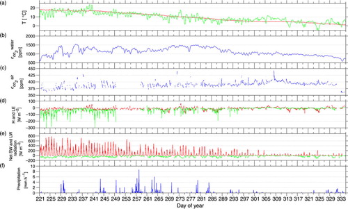
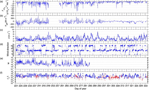
Fig. 3 Time series of half hour averages of (a) CO₂ flux (g CO₂ m⁻² s⁻¹), (b) the effective heat flux (W m⁻²), (c) wind speed (m s⁻¹), (d) wind direction, (e) Wedderburn number, and (f) atmospheric stability parameter (positive values are on red and negative on blue).

The components of the surface energy budget contributed in different ways to fall cooling. In general, the sensible heat flux was small, from −40 to 20 W m⁻² (Fig. 2d). The sensible heat flux tended to be negative with some positive values when the lake was warming, for example, on days 238–240, 273 and 306. With positive values, we indicate a flux to the lake, while negative values signal flux to the atmosphere. The latent heat flux (Fig. 2d) varied between −300 and 0 W m⁻² during the first month and became negligible when surface water temperatures were low. Maximum net shortwave radiation (Fig. 2e) was around 800 W m⁻² during daytime at the beginning of the measurements, then steadily declined to <50 W m⁻². The net longwave radiation (Fig. 2e) was always negative, occasionally up to −120 W m⁻², but on average −32 W m⁻². There were occasional rains (Fig. 2f), of which the most distinct event was the period of 2 weeks beginning on day 254. However, although it was raining every day during that time, the intensities were typically low, that is, <4 mm h⁻¹.

The CO₂ flux was negative all the time (Fig. 3a); that is, the lake was a source of CO₂ to the atmosphere. In the first half of the measurements, the flux varied in general between −10 and 0 g CO₂ m⁻² day⁻¹, with occasionally higher values. During the second half, the CO₂ effluxes tapered off, in general <3 g CO₂ m⁻² day⁻¹ after day 280. Overall, the CO₂ efflux was <7 g CO₂ m⁻² day⁻¹ about 90% of the time. The effective heat flux was largely negative during fall cooling with diel cycles of heating and cooling more common early in the study when solar radiation was higher (Fig. 2e, 3b). On average the effective heat flux was ca. −60 W m⁻² in the first half, and −30 W m⁻² during the second half of the study. The wind speed varied from 0.1 to 8.4 m s⁻¹ (Fig. 3c). About 50% of the time the speed was <1.6 m s⁻¹, 65% less than 2.0 m s⁻¹, and <3.0 m s⁻¹ about 85% of the time. There was significant channelling in the wind direction over the lake (Fig. 1); that is, 55% of the time the wind blew from the south (120°–180°) and 30% from the north (300°–360°), but there were periods when the wind rotated, for example, on days 222–226, 253–255 and 312–325 (Fig. 3d). Typical of these periods, wind speeds were also low. There were five periods of stronger winds when the wind speeds were close to or exceeded 6 m s⁻¹. Three of the most distinctive periods were in the second half of the study, the first on days 286 and 287, second on 291–293 and the last on 308–310. The Wedderburn number was calculated for the period of seasonal stratification (Fig. 3e), with, as expected, low values when wind speeds were high. Before day 255, when wind speeds were >4 m s⁻¹, W declined to <5, as is seen, for example, on days 221–222, 228, 233–234, 241 and 247, and on days 248–249 when U>5 m s⁻¹, W was <2. Values of L _N were slightly lower (data not shown) and supported the interpretation that internal wave induced mixing was likely whenever W<5. After day 255, as the lake continued to cool and the temperature gradient between epilimnion and hypolimnion reduced, W often dropped to <2 when winds rose >4 m s⁻¹, that is, on days 255–256, 258–259, 262, 265–267, 273–277, 279 and 283.

The stability parameter z _m /L (Fig. 3f), where L is the Monin-Obukhov length scale in the atmosphere, was typically between −2 (unstable conditions) and −0.01 (near-neutral conditions). There were some periods when the lake was heating and the z _m /L was positive, being then in general from 0.2 (slightly stable conditions) to 0.001 (neutral conditions). High heat loss co-occurred with low winds speeds at night early in the study, when the atmosphere above the lake was unstably stratified, and z _m /L was<−0.55. Most of these data at such times were discarded due to strict quality criteria. During periods of higher wind speed, near-neutral conditions (absolute value of z _m /L<0.05) were observed.

In early August, there was a strong seasonal thermocline between 5 and 9 m depth with temperature difference across it of about 8°C. The temperature in the upper mixed layer was about 18°C (Fig. 4a). The seasonal stratification decreased as the lake cooled, and the mixed layer deepened. The CO₂ concentrations in the mixing layer were around 800 ppm in the beginning of the measurements (Fig. 4b). There are four distinct periods of upwelling from the thermocline to the mixed layer on days 221–253. All of these events were related with W dropping to <5, and with concomitant cooling, the entrainment led to increased surface water CO₂ concentrations, as seen on days 228–229, 233–235, 241 and 248–251.

Fig. 4 (a) Isotherms (°C, 10-minute averages) and (b) isopleths of CO₂ concentrations (ppm) in the water column during seasonal stratification. The CO₂ data for 0–3 m are from Vaisala probes (0.5-hour averages) and for depths beyond that from headspace samples (weekly data). Temperatures were measured to a depth of 10 m, whereas the CO₂ measurements were to 11 m.

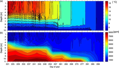
Concentrations of CO₂ in the surface water were variable. Increases were sometimes explained by upwelling, but at other times decreases occurred (e.g. day 258). One explanation could be dilution from rain fall. Alternatively, the decrease could be from advection. Wedderburn numbers dropped to 2 on day 256 and as the thermocline relaxes after such events, water from elsewhere in the basin can be advected into the measurement region contributing to variability in concentrations.

When the upper mixed layer deepened to over 8 m on day 266, the CO₂ rich hypolimnetic waters mixed with epilimnetic waters, and CO₂ concentrations increased to values >1400 ppm. After day 285 the whole lake water column was nearly isothermal, the water temperature was 7°C, and CO₂ concentrations had decreased such that values were close to 600 ppm in the water column before ice on in early December.

3.2. The measured and modelled gas transfer velocities

We used two approaches to calculate the k using the EC data. The first was with the measured surface CO₂ concentrations at the measurement site [eq. (1), Fig. 5a, dashed red line, k _site ], and the second was based on the estimated surface CO₂ concentrations in the EC footprint in which c _aq in eq. (1) are concentrations at depth z _E estimated from the Wedderburn number (Fig. 5a, solid blue line, k _fp ), see section 2.3 for details. Both k were high in the first half of the measurements, k _site being on average 7.5 cm h⁻¹ and k _fp 6.4 cm h⁻¹ and ranged from near zero to over 25 cm h⁻¹. As a response to diurnal heating and nocturnal cooling, effective heat flux and atmospheric CO₂ concentrations varied over diel cycles. During the stratified period, using CO₂ concentration from depth z _E reduced the number of times when k values were outside typical ranges (Banerjee and MacIntyre, 2004). We recorded during light winds 104 events with k _site when k>15, and only 49 similar events with k _fp . When heat flux declined and variability decreased after day 293, the variation in k was reduced. Values of both k _site and k _fp decreased towards the end of the measurements and were identical after day 285 when measured CO₂ concentrations were near uniform. Two example periods of measured and modelled k are discussed in more detail later.

Fig. 5 Half hour averages of (a) k _site (cm h⁻¹, red dashed line) and k _fp (solid blue line), (b) the aquatic friction velocity (blue line, m s⁻¹) and the convective velocity (green, m s⁻¹), and the wind parameter (blue) and the heat flux parameter (green) in k _Uw (c, 10⁶ m² s⁻²) and k _SR (d, 10¹² m⁴ s⁻⁴).

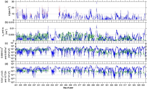
To determine conditions when buoyancy flux makes a considerable contribution to mixing relative to wind in the actively mixing layer, we contrasted convective and aquatic friction velocities (Fig. 5b). To determine whether buoyancy flux contributes appreciably to the gas transfer coefficient, we compared the wind shear term and the buoyancy term in our new model, k _Uw (Fig. 5c) and with the scaling in the surface renewal model, k _SR (Fig. 5d). Early in the study, u _*w and w _* were similar in magnitude (Fig. 5b). Typically, at night during the first half of the measurements, w _* was high, >0.004 m s⁻¹, and u _*w low, <0.002 m s⁻¹, indicating that convective mixing would distribute dissolved gases throughout the mixed layer. In the daytime, the buoyancy flux was typically positive and the w _* equalled zero by definition. When the heat flux decreased towards the end of the season, w _* was <0.002 m s⁻¹. During high wind events, the u _*w reached or exceeded 0.01 m s⁻¹, indicating wind was more effective in mixing as surface water temperatures cooled. The wind parameter in k _Uw was typically <0.5*10⁻⁶ m² s⁻², except when winds rose >5 m s⁻¹, resulting in values >10⁻⁶ m² s⁻², as seen on days 249, 280, 286, 292 and 332, and all these events were also visible as peaks in the k data. The heat flux parameter in k _Uw followed the pattern of convective velocity (Fig. 5b), and when the parameter values were high, for example, >0.15*10⁻⁶ m² s⁻² during days 240–249, also the k tended to be high, around 10 cm h⁻¹. Thus, with the scaling in k _Uw , the buoyancy flux term contributes to the gas transfer coefficient. The wind parameter in the surface renewal model responded to rising winds as seen for example, on days 249, 286 and 292 when winds of >7 m s⁻¹ resulted in parameter values reaching or exceeding 2*10⁻¹¹ m⁴ s⁻⁴. The heat flux parameter in k _SR also followed the pattern observed in w _* . However, it was always at least one order of magnitude smaller than the wind parameter, with only occasional exceptions very early in the study when both parameters were of equal magnitude. As a result of the different scaling, buoyancy flux had larger contribution in k _Uw than in k _SR . The accuracy in the different weighting approaches between k _Uw and k _SR are important for assessing the generality of the surface renewal model and will be discussed later.

Results from the models of k, that is k _Uw , k _SR , k _RA and k _CC [eqs. (12, 15, 18 and 17)], are contrasted with k _site and k _fp during stratified (Fig. 6) and unstratified (Fig. 7) conditions. Until day 244, the k _site and k _fp were almost identical, and the values were close to the modelled k. Prior to 244, winds were southerly with a diel cycle with stronger winds in the day and weaker winds at night and the lake gained heat at daytime, sometimes even over 200 W m⁻² and lost heat at night. On day 244, winds shifted to northerly and were steady for three days, U ~2 m s⁻¹. Also, the lake was cooling continuously. Lake numbers dropped to a value of 2 on day 244, and high frequency non-linear internal waves occurred in the upper thermocline between days 244 and 246. These waves are indicative of wind speeds relative to stratification being high enough to cause thermocline tilting. Concomitantly, the actively mixing layer deepened (Fig. 4a), indicating entrainment of metalimnetic waters to the surface. When measured surface CO₂ concentration was used in k calculations, many times very high k, k>15, were observed and the average value between days 244 and 247 was 10.7 cm h⁻¹ with k _site (Fig. 6, dashed line). When we assume that entrainment had occurred at the EC footprint and CO₂ concentrations had mixed and were equal to those at z _E , almost all the very high k were gone, and k _fp (Fig. 6, blue line) was similar to the values modelled, and the mean k dropped to 7.6 cm h⁻¹, which was nearer the modelled average of 5.4 cm h⁻¹ with k _Uw and k _SR .

Fig. 6 Half hour averages of k _site (black, dashed line, cm h⁻¹) and k _fp (blue line), and the modelled gas transfer velocities with k _Uw (green), k _SR (red), k _RA (turquoise) and k _CC (purple) during days 237–250.

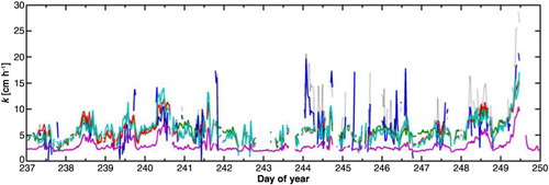
After this period, the winds started to rise, first reaching 5 m s⁻¹ on day 248 and then one of the highest winds measured in this study, over 8 m s⁻¹ on day 249. During both of these days, very high k were measured with k _site , but when the decrease in W and entrainment from convection was considered (Fig. 4b), k _fp was more similar to modelled k than k _site . Overall, the models k _Uw , k _SR and k _RA performed very similarly during this example period, whereas k _CC was about half of the other models’ estimates.

The second example (Fig. 7) is from late autumn (days 300–320), when the heat flux was already very low, around 30 W m⁻² from day 300 to 313, after which it dropped to about −50 W m⁻². During this period, with k _site and k _fp identical, the measured k followed the patterns observed in wind speeds, for example, as seen on days 300–301 and 308–310 (Fig. 3c, 7 blue line) and when strong winds of >4 m s⁻¹ prevailed, the measured k stayed high, >10 cm h⁻¹.

Fig. 7 Half hour averages of k _fp (blue line, cm h⁻¹), and the modeled gas transfer velocities with k _Uw (green), k _SR (red), k _RA (turquoise) and k _CC (purple) during days 300–320.

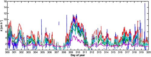
During the second example, k _Uw performed quite similarly to k _RA , and closely followed the measured k. The k _SR quite constantly overestimated the measured k by 2 cm h⁻¹ except in the event of high winds on days 309–310, when k _SR was close to the measured k. The k _CC was almost all the time <2 cm h⁻¹ with the exceptions at strong winds, for example, on days 309 and 310 when it rose to 4 cm h⁻¹. However, k _CC was still underestimating the measured k by a factor of 2.

With respect to the study as a whole, the models k _Uw , k _SR and k _RA performed similarly and the comparison was better with k _fp than with k _site . Virtually all of the very high k values with k _site were well above the modelled values, whereas when the CO₂ concentration correction from entrainment was accounted for in k _fp , many of the very high k decreased to the same range as the modelled k. This congruence supports our approach for estimating CO₂ concentrations in the EC footprint. The regression model, k _RA , and the surface renewal model had similar patterns to k _Uw and were more closely aligned when winds increased than during light winds with heat loss. Under such cases, k _Uw almost always provided the highest values, but regrettably these were also the occasions when most of the k data did not pass the quality tests and no reliable comparison could be made with the measured k. The k _CC was quite steadily ~2 cm h⁻¹, rising only when winds rose, and even during those conditions k _CC was lower by a factor of two relative to other modelled and measured k. The average value for k was 4.2, 5.5, 4.2 and 2.2 cm h⁻¹ with k _Uw , k _SR , k _RA and k _CC , respectively, and 6.0 and 5.2 with k _site and k _fp , respectively.

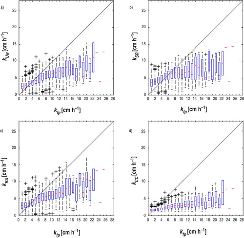
Comparisons of the modelled k against k _fp (Fig. 8) showed similar performance for k _Uw (Fig. 8a), k _SR (Fig. 8b) and k _RA (Fig. 8c) and two-fold higher modelled estimates than with k _CC (Fig. 8d). When k _fp was <8 cm h⁻¹, the relation to the modelled k (k _Uw , k _SR , k _RA ) was close to linear, with greater linearity under heating conditions (data not shown). Once k _fp exceeded 8 cm h⁻¹, the modelled k values were underestimations. The k _CC (Fig. 8d) underestimated k _fp essentially all the time. The higher k _fp relative to the models based on wind speed and buoyancy points either to the models not capturing an important aspect of the physics at the air–water interface or to continued underestimation of the CO₂ concentrations within the EC footprint.

Fig. 8 The k _fp (cm h⁻¹), 0.5 hour averages, plotted against (a) k _Uw , (b) k _SR , (c) k _RA and (d) k _CC . The central red line of the box is the median, the edges of the box the 25th and 75th percentiles, the whiskers show the extreme values (±2.7σ) and the black crosses are remaining outliers. The data were binned by k _fp , every 1 cm h⁻¹, and the bins from 1 to 7 contain about 200 data points, bins 8–13 about 100, bins 14–18 about 50, and bins 19–25 less than 20 data points.

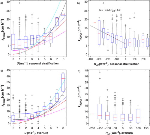
We obtained different relations for wind speed and k _600fp , k _fp after Schmidt number correction to CO₂ at 20°C, during the stratified and unstratified period, when heat flux was negligible. During the stratified period (Fig. 9a), median values and the 25 and 75% values for k _600fp showed a weak dependency on wind speed until winds reached 6 m s⁻¹, with median k _600fp from 5 to 9 cm h⁻¹. This pattern was evident for both heating and cooling conditions, but the median values were ~5 cm h⁻¹ under heating conditions and ~8 cm h⁻¹ under cooling conditions (data not shown). We obtained the same results using Lake numbers with their slightly larger predicted thermocline tilt (data not shown). The trend is similar to McGillis et al. (2004), which predicted high continuous k even at low winds. In contrast, during the unstratified period (Fig. 9c), the data showed a power law dependence similar to McGillis et al. (2001), with median k _600fp of 3 cm h⁻¹ for U<3 m s⁻¹. During seasonal stratification, k _600fp had a linear relation to the effective heat flux during cooling conditions, k _fp =−0.026H _eff +6.0 (Fig. 9b), and no relation during heating. During autumn overturn, when the heat fluxes were quite small, no trend was visible between H _eff and k _600fp (Fig. 9d).

Fig. 9 The k _600fp (cm h⁻¹), which is k _fp after Schmidt number conversion, plotted against wind speed (m s⁻¹) during (a) seasonal stratification (days 220–270) and (c) autumn overturn (days 290–335) and against the effective heat flux (W m⁻²) during (b) seasonal stratification and (d) autumn overturn. Also the regression of Cole and Caraco (1998) (purple line); Crusius and Wanninkhof (2003), k=0.168+0.228 (U ₁₀ )^2.2 (turquoise); Wanninkhof (1992), k=0.45(U ₁₀ )^1.64 (red); McGillis et al. (2001), k=3.3+0.026(U ₁₀ )³ (black) and McGillis et al. (2004), k=8.2+0.014(U ₁₀ )³ (blue) are presented in (a) and (c). The same statistical approach was used as in Fig. 8. In (a) and (c), the data were binned by wind speed, every 1 m s⁻¹, and the bins from 0 to 8 contain about 300, 800, 600, 400, 200, 100, 30, 10 and 5 data points, respectively. In (b) and (d), the data were binned by heat flux, every 50 W m⁻². The bins from −350 to 250 in (b) contain about 5, 10, 20, 50, 200, 400, 400, 200, 100, 50, 20, 10 and 10 data points, respectively, and the bins from −200 to 150 in (d) contain about 3, 50, 200, 500, 900, 100, 10 and 2 data points, respectively.

Evaluation of the relations between environmental parameters, the different models for k, and the k _fp with the Pearson correlation (Table 1) showed good comparisons between models and a strong influence of wind in all seasons. For the full period, the correlations of the various models with k _fp varied between 0.48 and 0.62 and were slightly higher than those with wind alone (Table 1). The correlations between the k _fp and effective heat flux, w _* and buoyancy flux were −0.47, 0.32 and −0.47, respectively, during cooling periods. All the models performed best during autumn overturn, when the correlation with k _fp was ~0.6, and the correlation between k _fp and wind speed was 0.61. The poorest correlations between the models and k _fp were during seasonal stratification, when the environmental drivers, wind speed and heat flux, had low correlations with k _fp , 0.29 and −0.32, respectively. Since there was a trend between heat flux and k _600fp (Fig. 8b), the low correlations were related to high scatter in k _fp , which was related to both the highly varying conditions within the lake ( Fig. 3e, 4) and EC random uncertainty, which is about 30% with 0.5-hour averaged CO₂ fluxes. Again, the k data were mostly discarded during high heat loss and low winds, which confounds the correlation between k _fp and heat loss expected from MacIntyre et al. (2010) and Read et al. (2012).

Table 1. The Pearson correlations between the measured k and the models (k _Uw , k _SR , k _RA and k _CC ), environmental forcing (wind speed, effective heat flux) and the parameters used in the models (aquatic friction velocity, convective velocity and buoyancy flux) during the whole measurement period, and separately during seasonal stratification and autumn overturn

	k Uw	k SR	k RA	k CC	U	u *	H eff	w *	β
k fp , overall	.62	.48	.58	.60	.49	.51	−.47	.32	−.47
k fp , seasonal stratification	.36	.33	.35	.30	.29	.32	−.32	.12	−.35
k fp , autumn overturn	.64	.59	.59	.68	.61	.62	−.23	.06	−.28

The correlations between k _fp and H _eff , w _* and β are only shown when the lake was cooling. All of the correlations were significant at the 0.01 level (two-tailed) except with w _* during autumn overturn. The N were 2150, 733 and 1029 for k _Uw , k _SR , k _RA , k _CC , U and u _* , and 1591, 536 and 783 for H _eff , w _* and β during the whole period, seasonal stratification and autumn overturn, respectively.

4. Discussion and conclusions

Our comparison of the relation between k ₆₀₀ and winds during the unstratified and stratified periods on Lake Kuivajärvi allows generalities which will apply to other lakes. During the unstratified period, the dependence on wind speeds occurred over a larger range of winds with the power law dependence greater than quadratic. These results point to turbulence controlling the gas transfer coefficient (Wanninkhof et al., 2009). The intercept for low winds is similar to the values in McGillis et al. (2001) and 50% higher than in Cole and Caraco (1998). During the stratified period, k ₆₀₀ did not depend on wind speed until winds reached approximately 6 m s⁻¹. The median k ₆₀₀ values were of order 6–9 cm h⁻¹ at wind <6 m s⁻¹, similar to that observed by McGillis et al. (2004). The k ₆₀₀ values depend also on the magnitude of buoyancy flux under cooling and are independent of buoyancy flux under heating. The combination of rigorous quality control of our EC data, and our derivation of k which includes modification of gas concentrations induced by thermocline upwelling led to improved estimates of k ₆₀₀ . Therefore, we conclude that the dependency of k ₆₀₀ on wind speed observed here and similar to observations in McGillis et al. (2001) is correct under unstratified conditions and stratified conditions with heating. In contrast, under cooling and for winds up to ~6 m s⁻¹, median k ₆₀₀ values were of order 7 cm h⁻¹. While these results are similar to observations of McGillis et al. (2004) in an oceanic study, it is uncertain whether the enhancement under cooling conditions was due to a stronger contribution of buoyancy flux than captured in our models or whether it was due to not fully capturing the spatial variability of CO₂ concentrations in the EC footprint. Our measured mean gas transfer velocity for the whole study period was k _site =6.0 cm h⁻¹, k _fp =5.2 cm h⁻¹, and k _Uw and k _RA were ~4 cm h⁻¹, that is, two times k _CC of 2.2 cm h⁻¹. These differences support recent work indicating results obtained using Cole and Caraco (1998) are underestimates (Rudorff et al., 2011), but see Schilder et al. (2013) and Vachon and Prairie (2013).

While wind was the dominant driver of the gas flux during overturn and at high winds, U>6 m s⁻¹, winds were <6 m s⁻¹ over 95% of the time. Our results indicate that there is uncertainty in estimates of k ₆₀₀ during cooling, and that continued effort to address this issue is required. Since low winds are a norm on small, sheltered lakes, and small lakes are orders of magnitude more abundant than large lakes (Downing et al., 2006), such effort is essential.

Our study indicates that Wedderburn numbers drop to values indicative of thermocline tilting and non-linear wave formation in small boreal lakes during fall cooling. Consequently, internal wave induced motions as well as convection from cooling deliver greenhouse gases as well as other dissolved substances to the upper mixed layer. Importantly, the resulting higher CO₂ flux is captured by EC technique where the flux, and inherently the spatial variability of CO₂ concentrations, from large areas is recorded. Thus, the EC technique, in contrast to chamber measurements, unless distributed over a lake surface, provides more accurate estimates of fluxes.

When lakes are stratified and internal waves moderate surface concentrations of greenhouse gases, accurate estimates of k depend on taking into account within lake physics when deriving k. When this effect was considered in k _fp using the Wedderburn number and actively mixing layer depth, the measured mean k was reduced about 13% and many of the very high k, values >15 cm h⁻¹, when neither wind nor heat loss indicated high k, decreased to values estimated with models which were independent from measured concentrations. Here we show, then, that the effects of wind and buoyancy flux at the surface mediate the gas transfer coefficient, and, when Wedderburn numbers drop to critical values, horizontal advection and vertical mixing from wind and buoyancy flux must be included in assessing fluxes of gases to the air–water interface. Consequently, focus should be put in developing more sophisticated, physically derived models and coupling these with biogeochemical models in order to develop generalities and for scaling up.

The mean CO₂ flux during seasonal stratification was 1.15 µmol m⁻² s⁻¹, which was about four times the flux measured on another Finnish lake (Vesala et al., 2006; Huotari, 2011) and on a lake in Switzerland (Eugster et al., 2003), and almost five times the average flux from Alaskan lakes (Kling et al., 1992). During autumn overturn, the mean CO₂ efflux was 0.56 µmol m⁻² s⁻¹, still higher than the efflux from the other lakes, indicating that boreal lakes surrounded by a managed forest might be an exceptionally high source of CO₂ during the whole open-water period.

The results presented here provide solutions for improved estimates of k using EC approaches. Accounting for the spatial variability of surface CO₂ concentrations allows for a more accurate derivation of k with the EC system. Here, we used a simple model of thermocline tilting due to decreases in the Wedderburn number below critical values. This approach significantly decreased the number and magnitude of high values of k. While other studies could similarly use this model, accuracy will be improved by measuring CO₂ concentrations at multiple sites. We are uncertain as to the extent of error with spatially variable cooling, but it can also contribute to uncertainty and should be included in models. By consideration of the within-water column physics, estimates of k as a function of wind and buoyancy flux will be improved allowing for greater accuracy in estimates at global scales.

5. Acknowledgements

This study was funded through the Academy of Finland Center of Excellence program (project 1118615), Academy of Finland ICOS project (263149), EU ICOS project (211574), Research Foundation of the University of Helsinki, EU GHG-Europe project (244122), EU-project GHG-LAKE, DEFROST (Nordforsk) project, Academy of Finland (project 218094), and University of Helsinki research funds through the project Vesihiisi. Funding was provided by U.S. National Science Foundation Grants DEB 0919603 and ARC 1204267 to SM. We thank H. Miettinen for practical help during the field activities and the staff of the Hyytiälä Forestry Field Station for invaluable assistance and friendly working atmosphere.

References

- Abril G , Martinez J. M , Artigas L. F , Moreira-Turcq P , Benedetti M. F , co-authors . Amazon River carbon dioxide outgassing fuelled by wetlands. Nature. 2013; 504: 395–398.
- Aubinet M , Vesala T , Papale D . Eddy Covariance. A Practical Guide to Measurement and Data Analysis. 2012; Dordrecht, The Netherlands: Springer.
- Banerjee S , MacIntyre S , Grue J , Liu P. L. F , Pedersen G. K . The air–water interface: turbulence and scalar exchange. Advances in Coastal and Ocean Engineering. 2004; World Scientific, Singapore. 181–237.
- Boegman L , Ivey G. N , Imberger J . The degeneration of internal waves in lakes with sloping topography. Limnol. Oceanogr. 2005; 50(5): 1620–1637.
- Cole J. J , Caraco N. F . Atmospheric exchange of carbon dioxide in a low-wind oligotrophic lake measured by the addition of SF6. Limnol. Oceanogr. 1998; 43: 647–656.
- Cole J. J , Prairie Y. T , Caraco N. F , McDowell W. H , Tranvik L. J , co-authors . Plumbing the global carbon cycle: integrating inland waters into the terrestrial carbon budget. Ecosystems. 2007; 171–184.
- Crill P. M , Bartlett K. B , Harriss R. C , Gorham E , Verry E. S , co-authors . Methane flux from Minnesota Peatlands. Glob. Biogeochem. Cycles. 1988; 2(4): 371–384.
- Crusius J , Wanninkhof R . Gas transfer velocities measured at low wind speed over a lake. Limnol. Oceanogr. 2003; 48(3): 1010–1017.
- Deacon E. L . Gas transfer to and across an air–water interface. Tellus. 1997; 29: 363–374.
- Downing J. A , Prairie Y. T , Cole J. J , Duarte C. M , Tranvik L. J , co-authors . The global abundance and size distribution of lakes, ponds, and impoundments. Limonol. Oceanogr. 2006; 51: 2388–2397.
- Eugster W , Kling G , Jonas T , McFadden J. P , Wüest A , co-authors . CO2 exchange between air and water in an Arctic Alaskan and midlatitude Swiss lake: importance of convective mixing. J. Geophys. Res. 2003; 108: 1–12.
- Fairall C. W , Hare J. E , Edson J. B , McGillis W . Parameterization and micrometeorological measurement of air–sea gas transfer. Boundary Layer Meteorol. 2000; 96: 63–105.
- Foken T , Wichura B . Tools for quality assessment of surface based flux measurements. Agr. Forest Meteorol. 1996; 78: 83–105.
- Hari P , Pumpanen J , Huotari J , Kolari P , Grace J , co-authors . High-frequency measurements of productivity of planktonic algae using rugged nondispersive infrared carbon dioxide probes. Limnol. Oceanogr. Methods. 2008; 6: 347–354.
- Horn D. A , Imberger J , Ivey G. N . The degeneration of large-scale interfacial gravity waves in lakes. J. Fluid Mech. 2001; 434: 181–207.
- Huotari J . Carbon Dioxide and Methane Exchange between a Boreal Pristine Lake and the Atmosphere. 2011; Helsinki University Print, Helsinki, Finland. Doctoral thesis.
- Imberger J . The diurnal mixed layer. Limnol. Oceanogr. 1985; 30: 737–770.
- Imberger J , Patterson J. C . Physical limnology. Adv. Appl. Mech. 1990; 27: 303–475.
- Jähne B , Haußecker H . Air–water gas exchange. Ann. Rev. Fluid Mech. 1998; 30: 443–468.
- Jähne B , Münnich K. O , Bösinger R , Dutzi A , Huber W , co-authors . On the parameters influencing air–water gas exchange. J. Geophys. Res. 1987; 1937–1949.
- Jeffery C. D , Woolf D. K , Robinson I. S , Donlon C. J . One-dimensional modelling of convective CO2 exchange in the Tropical Atlantic. Ocean Model. 2007; 19: 161–182.
- Jonsson A , Åberg J , Lindroth A , Jansson M . Gas transfer rate and CO2 flux between unproductive lake and the atmosphere in northern Sweden. J. Geophys. Res. 2008; 113: G04006.
- Kling G. W , Kipphut G. W , Miller M. C . The flux of CO2 and CH4 from lakes and rivers in arctic Alaska. Hydrobiologia. 1992; 240: 23–36.
- Kolari P , Kulmala L , Pumpanen J , Launiainen S , Ilvesniemi H , co-authors . CO2 exchange and component CO2 fluxes of a boreal Scots pine forest. Bor. Environ. Res. 2009; 14: 761–783.
- Kortelainen P , Rantakari M , Huttunen J. T , Mattsson T , Alm J , co-authors . Sediment respiration and lake trophic state are important predictors of large CO2 evasion from small boreal lakes. Glob. Chang. Biol. 2006; 12: 1554–1567.
- Launiainen S . Seasonal and inter-annual variability of energy exchange above a boreal Scots pine forest. Biogeosciences. 2010; 7: 3921–3940.
- Le Quéré C , Raupach M. R , Canadell J. G , Marland G , Bopp L , co-authors . Trends in the sources and sinks of carbon dioxide. Nat. Geosci. 2009; 2: 831–836.
- López Bellido J , Tulonen T , Kankaala P , Ojala A . CO2 and CH4 fluxes during spring and autumn mixing periods in a boreal lake (Pääjärvi, southern Finland). J. Geophys. Res. 2009; 114: G04007.
- MacIntyre S , Clark J. F , Jellison R , Fram J. P . Turbulent mixing induced by nonlinear internal waves in Mono Lake, California. Limnol. Oceanogr. 2009; 54(6): 2255–2272.
- MacIntyre S , Eugster W , Kling G. W , Donelan M. A , Drennan W. M , Saltzman E. S , Wanninkhof R . The critical importance of buoyancy flux for gas flux across the air–water interface. Gas Transfer at Water Surfaces, Geophysical Monograph Series. 2001; Washington, DC: American Geophysical Union. 135–139.
- MacIntyre S , Flynn K. M , Jellison R , Romero J. R . Boundary mixing and nutrient fluxes in Mono Lake, California. Limnol. Oceanogr. 1999; 44(3): 512–529.
- MacIntyre S , Jonsson A , Jansson M , Aberg J , Turney D. E , co-authors . Buoyancy flux, turbulence, and the gas transfer coefficient in a stratified lake. Geophys. Res. Lett. 2010; 37: 2–6.
- Mammarella I , Launiainen S , Gronholm T , Keronen P , Pumpanen J , co-authors . Relative humidity effect on the high-frequency attenuation of water vapor flux measured by a closed-path Eddy covariance system. J. Atmos. Ocean. Technol. 2009; 26: 1856–1866.
- McGillis W. R , Edson J. B , Hare J. E , Fairall C. W . Direct covariance of air–sea CO2 fluxes. J. Geophys. Res. 2001; 106: 16729–16745.
- McGillis W. R , Edson J. B , Zappa C. J , Ware J. D , McKenna S. P , co-authors . Air–sea CO2 exchange in the equatorial Pacific. J. Geophys. Res. Oceans. 2004; 109
- Monismith S. G . Wind-forced motions in stratified lakes and their effect on mixed-layer shear. Limnol. Oceanogr. 1985; 30(4): 771–783.
- Monismith S. G . An experimental study of the upwelling response of stratified reservoirs to surface shear stress. J. Fluid Mech. 1986; 171: 407–439.
- Nordbo A , Launiainen S , Mammarella I , Leppäranta M , Huotari J , co-authors . Long-term energy flux measurements and energy balance over a small boreal lake using eddy covariance technique. J. Geophys. Res. 2011; 116: 1–17.
- Raatikainen M , Kuusisto E . Suomen järvien lukumäärä ja pinta-ala [The number and surface area of the lakes in Finland]. Terra. 1990; 102: 97–110. [In Finnish with English summary].
- Raymond P. A , Hartmann J , Lauerwald R , Sobek S , McDonald C , co-authors . Global carbon dioxide emissions from inland waters. Nature. 2013; 503: 355–359.
- Read J. S , Hamilton D. P , Desai A. R , Rose K. C , MacIntyre S , co-authors . Lake-size dependency of wind shear and convection as controls on gas exchange. Geophys. Res. Lett. 2012; 39: L09405.
- Richey J. E , Melack J. M , Aufdenkampe A. K , Ballester V. M , Hess L. L . Outgassing from Amazonian rivers and wetlands as a large tropical source of atmospheric CO2 . Nature. 2002; 416: 617–620.
- Roland F , Vidal L. O , Pacheco F. S , Barros N. O , Assireu A , co-authors . Variability of carbon dioxide flux from tropical (Cerrado) hydroelectric reservoirs. Aquat. Sci. 2010; 72(3): 283–293.
- Rudorff C. M , Melack J. M , MacIntyre S , Barbosa C. C. F , Novo E. M. L. M . Seasonal and spatial variability of CO2 emission from a large floodplain lake in the lower Amazon. J. Geophys. Res. 2011; 116: G04007.
- Rueda F. J , MacIntyre S . Flow paths and spatial heterogeneity of stream inflows in a small multibasin lake. Limnol. Oceanogr. 2009; 54(6): 2041–2057.
- Schilder J , Bastviken D , van Hardenbroek M , Kankaala P , Rinta P , co-authors . Spatial heterogeneity and lake morphology affect diffusive greenhouse gas emission estimates of lakes. Geophys. Res. Lett. 2013; 40: 1–5.
- Soloviev A. V , Donelan M , Graber H , Haus B , Schlüssel P . An approach to estimation of near-surface turbulence and CO2 transfer velocity from remote sensing data. J. Marine Syst. 2007; 66: 182–194.
- Soloviev A. V , Schlüssel P . Parameterization of the cool skin of the ocean and of the air ocean gas transfer on the basis of modeling surface renewal. J. Phys. Oceanogr. 1994; 24: 1339–1346.
- Vachon D , Prairie Y. T . The ecosystem size and shape dependence of gas transfer velocity versus wind speed relationships in lakes. Can. J. Fish. Aquat. Sci. 2013; 70: 1–8.
- Vachon D , Prairie Y. T , Cole J. J . The relationship between near-surface turbulence and gas transfer velocity in freshwater systems and its implications for floating chamber measurements of gas exchange. Limnol. Oceanogr. 2010; 55(4): 1723–1732.
- Vesala T , Eugster W , Ojala A , Aubinet M , Vesala T , Papale D . Eddy covariance measurements over lakes. Eddy Covariance. A Practical Guide to Measurement and Data Analysis. 2012; Dordrecht, The Netherlands: Springer. 365–376.
- Vesala T , Huotari J , Rannik Ü , Suni T , Smolander S , co-authors . Eddy covariance measurements of carbon exchange and latent and sensible heat fluxes over a boreal lake for a full open-water period. J. Geophys. Res. 2006; D11101.
- Wanninkhof R . Relationship between gas exchange and wind speed over the ocean. J. Geophys. Res. 1992; 97: 7373–7381.
- Wanninkhof R , Asher W. E , Ho D. T , Sweeney C , McGillis W. R . Advances in quantifying air–sea gas exchange and environmental forcing*. Ann. Rev. Mar. Sci. 2009; 1: 213–244.
- Zappa J. C , McGillis W. R , Raymond P. A , Edson J. B , Hintsa J , co-authors . Environmental turbulent mixing controls on air–water gas exchange in marine and aquatic systems. Geophys. Res. Lett. 2007; 34: L10601.