Modelling the response of stable water isotopes in Greenland precipitation to orbital configurations of the previous interglacial

Abstract

The relation between δ ¹⁸O of precipitation and temperature has been used in numerous studies to reconstruct past temperatures at ice core sites in Greenland and Antarctica. During the past two decades, it has become clear that the slope between δ ¹⁸O and temperature varies in both space and time. Here, we use a general circulation model driven by changes in orbital parameters to investigate the Greenland δ ¹⁸O–temperature relation for the previous interglacial, the Eemian. In our analysis, we focus on changes in the moisture source regions, and the results underline the importance of taking the seasonality of climate change into account. The orbitally driven experiments show that continental evaporation over North America increases during summer in the warm parts of the Eemian, while marine evaporation decreases. This likely flattens the Greenland δ ¹⁸O response to temperature during summer. Since the main climate change in the experiments occurs during summer this adds to a limited response of δ ¹⁸O, which is more strongly tied to temperature during winter than during summer. A south–west to north–east gradient in the δ ¹⁸O–temperature slope is also evident for Greenland, with low slopes in the south–west and steeper slopes in the north–east. This probably reflects the proportion of continental moisture and Arctic moisture arriving in Greenland, with more continental moisture in the south–west and less in the north–east, and vice versa for the Arctic moisture.

• stable water isotopes
• modelling
• moisture source
• seasonality
• previous interglacial

To access the supplementary material to this article, please see Supplementary files under Article Tools online.

1. Introduction

A major motivation for reconstructing past changes in Greenland ice sheet (GIS) elevation is to quantify the contribution to sea level changes owing to run-off from the GIS. The sea level is predicted to rise by 0.3–1.0 m by the end of the 21st century depending on emission scenario, although some semi-empirical studies estimate the upper range of sea level rise as being higher (Church et al., 2013). As the largest continental water reservoirs, melt from the ice sheets of Greenland and Antarctica is a major contribution to the predicted sea level rise. Presently, studies of the current mass balance of the GIS and the Antarctic ice sheet (AIS) show a net mass loss from both ice sheets, which is probably accelerating (Rignot et al., 2011; Van den Broeke et al., 2011; Shepherd et al., 2012). Records of past Holocene sea level show an increase of 3–5 m during the past 7000 yr (Fleming et al., 1998), during which GIS experienced only a moderate thinning (Vinther et al., 2009). This points to a contribution of melt from AIS during Holocene. During the Eemian, the sea level is estimated to have been up to 6–9 m higher than present (Kopp et al., 2009). Ice flow modelling studies suggest a substantial reduction of GIS during the Eemian, with the southern dome partly, or completely collapsed (e.g. Cuffey and Marshall, 2000; Otto-Bliesner et al., 2006; Helsen et al., 2013). However, studies of Greenland deep ice cores support that Eemian ice is present at the Dye-3 site in southern Greenland, although the elevation of the southern dome may well have been reduced by 400 m relative to other ice core sites (Johnsen and Vinther, 2007). Furthermore, studies of sediment discharge off Southern Greenland indicate that, although the ice sheet was probably reduced compared to Holocene, the Southern Greenland terrain was ice covered during the Eemian (Colville et al., 2011). Also, DNA studies suggest that the Dye-3 site has not been ice free for the last 450 kyr (1000 yr before present) (Willerslev et al., 2007). It is therefore likely that melt from AIS also contributed significantly to the Eemian sea level high-stand. In Antarctica, the western part of the ice sheet is believed to be very sensitive to changes in sea ice (Rignot and Jacobs, 2002). Warmer waters around Antarctica could have led to instability of the West Antarctic Ice Sheet (WAIS), and a collapse of WAIS could explain a sea level rise of the order of magnitude as that of the Eemian (Oppenheimer, 1998). The timing of the Eemian high-stand is not well established and there is some evidence (from the Yucatan peninsula, Mexico, and Western Australia) that the sea level did not reach its peak until after 121 kyr, where a sudden jump in sea level might have occurred (Blanchon et al., 2009; O'Leary et al., 2013). However, due to glacio-hydro isostatic processes it is risky to interpret individual records as proxies for global sea level (Lambeck et al., 2012).

Since the pioneering work of W. Dansgaard, relating the isotope ratio of precipitation to climate variables (e.g. Dansgaard, 1953), and recovery of the Camp Century ice core (Dansgaard et al., 1969), ice cores have been an important archive for past climate changes. The ratios of H₂ ¹⁸O/H₂ ¹⁶O and HD¹⁶O/H₂ ¹⁶O in precipitation, also written δ ¹⁸O and δD when expressed as the relative deviation from the SMOW standard (Craig, 1961), are linearly related to the local temperature at high latitude sites (e.g. Dansgaard, 1964). This has been exploited to translate the δ ¹⁸O of ice cores into temperature (e.g. Johnsen et al., 1992). Over the past two decades, it has become clear that the isotope–temperature slope used for calibrating ice core derived temperature variations back in time varies in both time and space. Notably, the temporal slope for δ ¹⁸O differs from the classical spatially derived Greenland isotope–temperature slope of 0.67‰/°C (Johnsen et al., 1989), with the temporal slope mostly being found to be lower than the spatial slope on annual, decadal and up to millennial time scales (Cuffey et al., 1992; Shuman et al., 1995, 2001; Johnsen et al., 2001). On glacial–interglacial timescales, the isotope–temperature slope is thought to be affected by precipitation weighting, due to limited winter precipitation during cold stages (Werner et al., 2000; Masson-Delmotte et al., 2005).

Simulations of the previous interglacial, the Eemian, and warm climate states (forced with 2×CO₂ and 4×CO₂ relative to preindustrial levels), using a general circulation model (GCM) with stable water isotope diagnostics, suggests that the Greenland isotope–temperature slope may be as low as 0.3‰/°C (Masson-Delmotte et al., 2011). However, a recent study by Sime et al. (2013) of the isotope–temperature relation for warm climate states shows a range of the Greenland isotope–temperature slope of 0.3–0.7‰/°C depending on the sea surface temperature (SST) and Arctic sea ice configuration for greenhouse gas (GHG) forced experiments. High Arctic SSTs and low sea ice concentration leads to a larger contribution of Arctic moisture, which gives a steeper isotope–temperature slope due to isotopically heavy high latitude water vapour and shorter distillation path. Using GHG driven model experiments as analogies for the Eemian climate, as chosen for the studies mentioned above, could be problematic as the climate response to changes in orbital parameters differs vastly in seasonality and spatial patters to the climate response to changes in GHG levels (Masson-Delmotte et al., 2011). The reason for choosing GHG driven simulations as analogies for the Eemian climate despite this concern, is the general underestimated modelled amplitude in temperature and δ ¹⁸O when comparing orbitally driven models with proxy records (Sime et al., 2013).

While the isotope–temperature slope during the Holocene can be calibrated using borehole temperature (Vinther et al., 2009), this is not feasible for the Eemian as palaeo-temperatures are not preserved in the ice sheet for this period. This means that, unless alternative methods for estimating Eemian palaeo-temperatures for Greenland are developed, modelling could be the best way to constrain the isotope–temperature relation during the Eemian.

A relative low sensitivity of δ ¹⁸O to temperature during warm climates would mean that a greater proportion of the δ ¹⁸O anomalies in ice cores for these periods could be interpreted as changes in ice sheet elevation. Examples of using δ ¹⁸O anomalies to infer changes in ice sheet elevation are Vinther et al. (2009) and Dahl-Jensen et al. (2013). This requires a separation of the isotope anomaly in the part owing to climate and circulation change and the part owing to local elevation change. A prerequisite to this separation is assuming an elevation–isotope slope (altitude effect or isotopic lapse rate) and an isotope–temperature slope. Ice sheet elevation can also be estimated using the total gas content of an ice core (Raynaud et al., 1997). However, the total gas content depends on temperature and insolation, which introduces some uncertainty (Raynaud et al., 2007).

So far, the isotopic altitude effect has only been calculated from present-day surface data (e.g. Dansgaard, 1961). Again, as for the traditional interpretation of the spatial isotope–temperature slope, this is a present-day spatial relation assumed to hold for temporal changes. This neglects any effect that changing the ice sheet elevation might have on atmospheric circulation, and in turn how this affects precipitation patterns and ultimately the isotopic composition.

Eemian ice has been recovered at several sites in Greenland, most notably at the NorthGRIP and NEEM ice core sites (Andersen et al., 2004; Dahl-Jensen et al., 2013). Both of these sites have δ ¹⁸O anomalies of ~+3‰. At the NorthGRIP site the Eemian δ ¹⁸O anomaly is interpreted as a change of at least +5°C (Andersen et al., 2004). This is based on the assumption that the modern spatial isotope–temperature slope of about 0.7‰/°C for Greenland is the upper limit for the temporal slope, and in turn gives the lower limit for the reconstructed temperature anomaly. For the NEEM site the Holocene isotope–temperature slope of 0.5‰/°C based on borehole temperature, also discussed above, was used for the Eemian temperature reconstruction. This, together with a slightly higher site elevation compared to present based on total gas content, gives a temperature anomaly of +8±4°C (Dahl-Jensen et al., 2013). As already mentioned, climate models run under Eemian conditions fail to reproduce these anomalies for both temperature and δ ¹⁸O.

The Arctic interglacial climate is governed by Earth's orbital configuration and a number of feedback mechanisms. While the mean annual insolation of the high latitudes is decided by the obliquity, the intensity of the summer insolation is also determined by the precession modulated by the eccentricity. The summer temperature is one of the primary parameters for the surface mass balance of ice sheets (e.g. Quiquet et al., 2012). During the early Eemian (126–130 kyr) Northern Hemisphere (NH) summers were shorter and warmer compared to the late Holocene due to changes in insolation caused by the orbital configuration (Braconnot et al., 2008). This is also indicated by Fig. 1, where the monthly insolation for 65°N is shown for present day and three time periods during the Eemian. Opposed to now, the NH summer was during perihelion when the Earth is closest to the Sun. Although the autumn/winter insolation was reduced to the same extent as the increase in summer insolation, it is likely that a number of feedback mechanisms caused the summer warming to be amplified and the overall climate to be warmer than present. Proxy data support that the warming during the Eemian was amplified in the polar region (Anderson et al., 2006), which is in-line with the theory of polar amplification of climate change (Alexeev et al., 2005). Large changes in sea ice cover (Norgaard-Pedersen et al., 2007; Adler et al., 2009) and vegetation (Schurgers et al., 2007) probably affected the Arctic environment on a local and regional scale.

Fig. 1 (a) Monthly top of the atmosphere (TOA) shortwave radiation (SWR) [Wm⁻²] at 65°N for control run (ctrl), 115k, 122k and 126k calculated following Berger (1978). (b) TOA SWR anomalies at 65°N for Eemian time slices.

In this model study, we focus on the isotope–temperature relation for Greenland and Arctic climate anomalies during the Eemian. The results for three Eemian time slices reflect the orbitally driven changes for the atmosphere, ocean and sea ice. Our experiment setup does not include changes in vegetation or ice sheets. We first introduce the model setup, then present the modelled NH and Arctic anomalies for temperature and δ ¹⁸O. Next, we present the isotope–temperature relation for Greenland in our model experiments and analyse the factors leading to this relation. Our analysis emphasises the effect of seasonality, and the influence of orbitally driven evaporation patterns on the isotope–temperature slope. In the end, we discuss our results in the context of other recent Eemian isotope model and ice core studies, and offer some perspectives on how to proceed with future studies.

2. Methods

Here we first give a summary of the model setup, followed by technical details on the model and boundary conditions used in our experiments. Further details on the model setup are listed in Table 1. We use the isotope enabled version of the of the European Centre Hamburg Model version 4 (ECHAM4-iso) in a T42 spectral resolution corresponding to a horizontal regular grid resolution of ~2.8°×2.8°, and a vertical resolution of 19 levels (Werner et al., 2000). After spin-up, the model is run in four 10 yr climatological experiments: a pre-industrial control (ctrl) and three time slices for 115, 122 and 126 kyr (115k, 122k, 126k). For each time slice, corresponding climatological monthly mean SST data of the IPSL_CM4 coupled atmosphere–ocean experiments for the Eemian are used as input (Braconnot et al., 2008). We calculate variations in orbital parameter following Berger (1978) with the vernal equinox fixed to March 21. As GHG levels varied relatively little for the time periods in question for this study (Fischer et al., 1999; Loulergue et al., 2008; Schilt et al., 2010), and we wish to focus on the effects of orbital forcing, we keep the GHG level constant between the time slices. Furthermore, present day ice sheets and vegetation are used for all time slices. In summary, the only boundary conditions and forcings that are changed between the experiments are orbital parameters and SSTs.

Table 1. Summary of boundary conditions for ECHAM4-iso simulations indicating source of sea surface temperature (SST), atmospheric CO₂ [ppmv], CH₄ [ppmv] and N₂O [ppbv] concentration, eccentricity (Ecc.) [°], obliquity (Obl.) [°], precession (Pre.) [o(ω−180°)], glacier mask (Glac.) and vegetation mask (Vege.)

Time slice	SST	CO2	CH4	N2O	Ecc.	Obl.	Pre.	Glac.	Vege.
Ctrl	IPSL_CM4 control	280	1.72	310	0.0167	23.4	102	Present	Present
115k	IPSL_CM4 115 kyr	280	1.72	310	0.0414	22.4	111	Present	Present
122k	IPSL_CM4 122 kyr	280	1.72	310	0.0407	23.2	356	Present	Present
126k	IPSL_CM4 126 kyr	280	1.72	310	0.0397	23.9	291	Present	Present

Since the IPSL_CM4 coupled model is used to produce the SST data driving the ECHAM4-iso, any biases of IPSL_CM4 in SSTs will be transferred to our simulations. We will briefly discuss the most notable biases and any relevance there may be to our results. The IPSL_CM4 has a low bias in Arctic sea ice in both summer and winter on the order of 10⁶ km², with the largest bias during summer (Marti et al., 2006). This is coupled with a warm bias in the Arctic SSTs. Furthermore, sea ice is binary in the ECHAM4 model, i.e. an ocean point is either ice covered or ice free. In our model runs, we define all ocean grid points with a SST below −1.8°C as being ice covered. This procedure is simple, but creates a bias towards too little sea ice. However, this mainly has a local effect at the sea ice margin. Another notable bias of IPSL_CM4 is a cold bias of ~−5°C in the North Atlantic SSTs covering the area 40–50°N (Swingedouw et al., 2007). The biases can affect the patterns of precipitation, evaporation and atmospheric circulation, for example by too warm (cold) SSTs leading to too high (low) evaporation rates. However, our analysis mainly focuses on anomalies between the control run and the Eemian time slices, under the assumption that the effect of the biases will cancel out. Of course, we cannot exclude that the biases can have non-linear effects. For example, if sea ice extent is underestimated in a given region, there is a limited effect of removing all sea ice compared to going from completely ice covered to ice free conditions.

The second order parameter deuterium excess (hereafter d-excess) is not a part of this study, despite the wide use of the d-excess as diagnostic for source area conditions (e.g. Johnsen et al., 1989; Masson-Delmotte et al., 2005; Steffensen et al., 2008). In our simulations, the d-excess is correlated to the δ ¹⁸O for GIS with a negative slope (R ²=0.4–0.5 for monthly values). The main spatial variations and anomalies during the Eemian time slices can be attributed to this relation. We ran the simulations with a moderate cloud supersaturation (Si=1–0.002·T), which results in overestimated d-excess values for low δ ¹⁸O values. It has been suggested by several studies that a higher supersaturation for low temperatures (e.g. Si=1–0.004·T) results in a better agreement with the observed d-excess–δ ¹⁸O relation for Antarctica (Schmidt et al., 2005; Risi et al., 2010; Werner et al., 2011). Higher supersaturation yields lower d-excess due to the effective fractionation factors of HD¹⁶O and H₂ ¹⁸O being more similar than for lower supersaturation. Since the d-excess–δ ¹⁸O relation dominates the d-excess variations in our simulations, further analysis of the modelled d-excess could lead to false conclusions. Also, the length of the simulations (10 yr) results in poor statistics for the d-excess, which has a low signal to noise ratio.

Before proceeding to the results, the reader should note that unless otherwise stated, all mapped model output is displayed in the original model resolution.

3. Results

We begin the results section with a brief review of the model performance over Greenland. Our control run produces realistic temperatures over GIS. For the GRIP ice core drill site, the modelled annual mean T_2m is −34°C, which is slightly lower than the present observed annual mean air temperature of −32°C (Johnsen et al., 1992). The lower modelled temperature could be explained by the preindustrial CO₂ level of our simulation, which naturally produces a generally cooler climate than the observed. Due to resolution, the ice sheet orography is smoothed in the model, resulting in overestimated temperatures towards the ice sheet margin and over southern Greenland. The performance of ECHAM4–iso simulations in T42 resolution over Greenland are also discussed by Sjolte et al. (2011).

3.1. Eemian Arctic anomalies for temperature and precipitation

The overall climate change between the three modelled Eemian time slices is a decrease of the NH summer temperatures going from 126k to 122k to 115k, and corresponding increase in winter temperatures (see Fig. 2). This can also be explained as a decrease in the amplitude of the annual cycle of temperature in response to the changing orbital parameters. For the Arctic region there is a strong response in sea ice, with a decrease in sea ice extend during summer that does not recover during winter. This means that there is a warming in the Arctic all year round despite decreased winter insolation. The Arctic warming affects the circumpolar region, including Greenland. In terms of temperature there is no cooling over GIS during winter (mean temperature above 1500 m) for 126k, while summer temperature anomalies peak in July with +6°C. The annual mean temperature anomaly for GIS above 1500 m is +1°C for 126k.

Fig. 2 Modelled JJA, DJF and annual mean 2m temperature (T_2m ) anomalies north of 45°N for the 115k time slice (a) to (c), 122k time slice (d) to (f) and the 126k time slice (g) to (i).

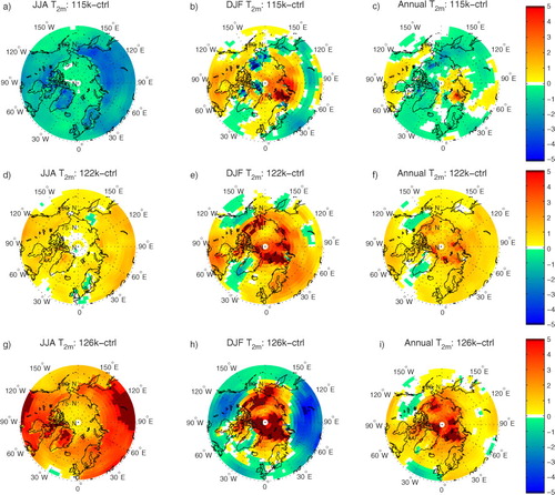
The general pattern of the modelled summer warming for 126k is +4–5°C over the Asian continent and North America, with smaller anomalies of +2–3°C over Northern Europe and Alaska. This agrees well with the CAPE proxy synthesis of Eemian peak summer temperatures (Anderson et al., 2006). However, a direct comparison with the proxy based annual mean temperatures by Turney and Jones (2010) reveals strongly underestimated modelled anomalies, both for continental and marine regions (not shown). Although the modelled SST anomalies (from IPSL_CM4) qualitatively reproduce the pattern of warming in high latitude and equatorial regions, with little or no change in the mid-latitudes, the warming is underestimated by a factor of 4. The proxy records have up to +8°C anomalies in the high northern latitudes, while the model only has up to +2°C anomalies in the annual mean SST. The same underestimation of continental temperatures by the model is clear, although the spatial coverage of the continental temperature proxies is limited compared to the marine coverage. The underestimated modelled Eemian temperature anomalies is a well-known discrepancy also discussed by Sime et al. (2009, 2013) and Lunt et al. (2013). This will be discussed further in Section 4. It should be noted that there is large spread in proxy data with examples of scattered positive and negative anomalies within close proximity of each other, which points to large uncertainties in the proxy based temperatures.

For GIS, there is no significant difference in annual mean precipitation amount between the different time slices (see Table 2). For the winter season, there is a slight decrease in precipitation over southern Greenland for 122k and 126k (not shown). This is most likely due to less storm activity over the Atlantic caused by a weaker latitudinal temperature gradient. The temperature gradient is weakened because of warmer Arctic temperatures, due to reduced sea ice, and colder mid-latitudes, due to less winter insolation.

Table 2. Absolute and anomalous GIS annual mean surface temperature [°C], annual mean precipitation weighted δ ¹⁸O [‰] and annual mean precipitation amount [mm/yr] above 1500 m for control run and Eemian time slices

Experiment	T surf	δ ^18O	Precip.	T surf anomaly	δ ^18O anomaly	Precip. anomaly
Ctrl	−26.7±0.6	−27.3±1.0	210±34	N/A	N/A	N/A
115k	−27.4±0.9	−27.6±0.9	201±34	−0.7	−0.2	−10
122k	−26.7±0.9	−27.4±1.0	209±41	0.0	0.0	−2
126k	−25.7±0.9	−26.8±0.9	201±39	0.9	0.5	−10

Absolute values are listed±one standard deviation.

3.2. Eemian δ ¹⁸O anomalies and the δ ¹⁸O-temperature relation for Greenland

The δ ¹⁸O anomalies over GIS are relatively small with an annual mean of ~+0.5‰ for 126k above 1500 m (see Table 2). This is slightly less than the 126 kyr anomalies of ~+0.75‰ produced by the LMDZ–iso model (Masson-Delmotte et al., 2011). Again, both of these models underestimate the anomalies of ~+3‰ found in Greenland ice cores, as also discussed in Section 1. The underestimated anomalies could be due to the fixed ice sheet elevation in the model runs, missing ice sheet run-off or other climate feedbacks. We will return to these issues in Section 4.

Monthly anomalies range from just under +2‰ during summer with winter values within ±1‰ (see also Fig. 3). If we take a look at the monthly values for June to August for GIS above 1500 m, the median of the simulated temperature in the control experiment of −14°C is shifted to −8°C in 126k, whereas there is no shift in the median of the simulated δ ¹⁸O value (−22‰) (see Fig. 4). Also, during summer the spatial pattern of the δ ¹⁸O anomalies correspond poorly to the temperature anomalies compared to the winter anomalies (see Table 3), with low spatial correlations in particularly for 122k and 126k. While this agrees with the general understanding of the Greenland δ ¹⁸O as a winter signal (Vinther et al., 2010; Sjolte et al., 2011) it does not offer an explanation for the pattern of the δ ¹⁸O anomalies.

Fig. 3 Modelled JJA, DJF and annual mean precipitation weighted δ ¹⁸O anomalies north of 45°N for the 115k time slice (a) to (c), 122k time slice (d) to (f) and the 126k time slice (g) to (i).

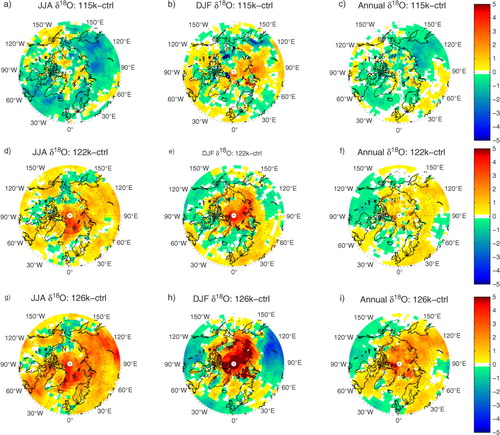
Fig. 4 (a) Histogram of monthly 2m temperature (T_2m ) over Greenland above 1500 m for the control run (ctrl) during JJA (black) and DJF (grey). (b) Histogram of monthly δ ¹⁸O in precipitation over Greenland for the control run (ctrl) during JJA (black) and DJF (grey). (c) and (d) same as (a) and (b) but for the 126k time slice.

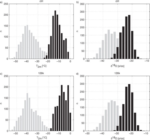
Table 3. Seasonal spatial slope (JJA and DJF means) and correlation (R ²) between δ ¹⁸O and temperature for land grid points north of 50°N (n=724) and for GIS above 1500 m (n=43)

Experiment	Slope >50°N (JJA)	Slope >50°N (DJF)	Slope of anomalies >50°N (JJA)	Slope of anomalies >50°N (DJF)	Slope GIS >1500 m (JJA)	Slope GIS >1500 m (DJF)
Ctrl	0.58±0.01 (0.92)	0.45±0.01 (0.78)	N/A	N/A	0.53±0.03 (0.91)	0.62±0.04 (0.87)
115k	0.58±0.01 (0.92)	0.46±0.01 (0.78)	1.14±0.07 (0.25)	0.51±0.02 (0.37)	0.56±0.04 (0.84)	0.61±0.04 (0.87)
122k	0.57±0.01 (0.90)	0.46±0.01 (0.78)	2.26±0.41 (0.04)	0.53±0.02 (0.48)	0.48±0.03 (0.90)	0.64±0.04 (0.87)
126k	0.58±0.01 (0.88)	0.46±0.01 (0.73)	0.48±0.06 (0.09)	0.65±0.02 (0.63)	0.50±0.03 (0.86)	0.55±0.04 (0.83)

Calculating the δ ¹⁸O–temperature slope based on the control run and the three Eemian time slices gives an estimate of the temporal slope. It should be taken into account that the calculation is only based on four data pairs, and care should be taken into interpreting the results considering the poor statistics. The slope for mean annual temperature and precipitation weighted δ ¹⁸O above 1500 m is 0.47‰/°C (R ²=0.96). This is calculated using the numbers in columns five and six of Table 2. The slope is steeper than the 0.3–0.4‰/°C for Eemian and CO₂-driven experiments of Masson-Delmotte et al. (2011), calculated in the same way as for our simulations, and within the 0.3–0.7‰/°C range by Sime et al. (2013), calculated between a control run and individual experiments with different SST configuration and GHG forcing. To assess regional differences in the slope, we calculated the slope for each grid point over Greenland. This is shown in Fig. 5. There is a south–west to north–east gradient in the low slopes in the south–west and steep slopes in the north–east. In the south, negative slopes are found and in the central-east GIS, a local maximum is found with slopes of more than 1‰/°C. By precipitation weighting the temperature, the effect of changes in the annual cycle of precipitation can be eliminated. The main pattern of the south–west to north–east gradient in the slopes is maintained and the scatter in the slopes is reduced. The local maximum in slopes in the central-east GIS disappears, meaning that this feature is caused by precipitation weighting of the isotopes. In Table 4 the seasonal (JJA and DJF) and annual slopes are listed for a number of ice core sites with isotope records reaching back to the Eemian (Johnsen and Vinther, 2007; Dahl-Jensen et al., 2013). The summer slopes are generally lower compared to winter; however, the winter slopes are very scattered showing a large range and very low δ ¹⁸O–temperature correlations. The scattered slopes during winter are most likely due to a low signal–noise ratio, as the temperature anomalies are small (generally within ±1°C). For the annual mean the slope varies from −0.45‰/°C at Dye-3 to 1.08‰/°C at GRIP; however, the fairly robust negative slope at Dye-3 flattens out when taking precipitation weighting into account. In general, the slopes calculated using the precipitation weighted temperature are significantly lower than the observed spatial slope of 0.67‰/°C, except at Renland where the slope is 0.86‰/°C.

Fig. 5 (a) Slope between annual mean precipitation weighted δ ¹⁸O and annual mean temperature (T_2m ) [‰/°C] calculated between the anomalies of the 115k, 122k and 126k time slices (b) one standard deviation on δ ¹⁸O–T_2m slope (c) linear correlation of δ ¹⁸O and T_2m between the time slices. (d) to (f) same as (a) to (c) but calculated using precipitation weighted annual mean T_2m . The asterisk mark the ice core drill sites listed in Table 4 [Camp Century (C), NEEM (N), NorthGRIP (NG), GRIP (G), Renland (R) Dye-3 (D3)].

Table 4.  δ ¹⁸O–temperature slope between Eemian time slices (115k, 122k, 126k) for ice core drill sites where Eemian ice has been recovered

Site	JJA [‰/°C]	DJF [‰/°C]	Annual [‰/°C]	Pre. w. annual [‰/°C]
Camp century	0.08±0.04 (0.52)	0.04±0.08 (0.09)	0.04±0.02 (0.02)	0.11±0.09 (0.33)
NEEM	0.07±0.05 (0.32)	0.56±0.04 (0.99)	0.35±0.12 (0.74)	0.14±0.04 (0.79)
NGRIP	0.29±0.08 (0.82)	8.27±41.59 (0.01)	0.61±0.04 (0.98)	0.26±0.00 (1.00)
GRIP	0.47±0.04 (0.98)	−0.08±0.02 (0.88)	1.08±0.33 (0.78)	0.41±0.03 (0.98)
Renland	0.23±0.01 (0.99)	1.86±0.13 (0.99)	0.55±0.11 (0.89)	0.86±0.06 (0.98)
Dye-3	0.25±0.10 (0.70)	1.35±0.64 (0.60)	−0.45±0.12 (0.82)	−0.15±0.09 (0.46)

The slope is listed for JJA and DJF means, annual mean precipitation weighted δ ¹⁸O with annual mean 2m temperature (Annual) and annual mean precipitation weighted δ ¹⁸O with annual mean precipitation weighted 2m temperature (Pre. w. annual). R ² listed in parenthesis. The ice core drill sites are marked in Fig. 5.

3.3. Moisture source areas: annual cycle of evaporation in moisture sources and regional differences for Greenland

Vapour tagging done by Werner et al. (2001) using ECHAM4–iso shows that the two most important present day moisture sources for the Summit region is the Atlantic and North American region. The results with ECHAM4–iso of Werner et al. (2001) further shows the dominance of North American moisture for Greenland during summer. The North Atlantic and Arctic are prevailing moisture sources during winter. At the same time, there is a spatial gradient in moisture sources where the influence of North American moisture is strongest in the south–west, North Atlantic moisture is strongest in the south–east and Arctic moisture is strongest in the north and along the coast. Similar results are achieved by Sime et al. (2013) using HadAM3 and LMDZ4, although the Arctic is suggested to be a stronger moisture source in Eastern Greenland. These results are model dependent and are also not directly comparable due to the definitions of the different source areas.

For our experiments, moisture tagging is not available. However, we have performed the following analysis of vapour advection, humidity levels, isotopic composition of vapour, as well as isotopic composition and rates of evaporation for the moisture source areas discussed above.

In response to the insolation anomalies during summer, NH continental evaporation is increased for 122k and 126k, while it is decreased for 115k. Seasonal evaporation anomalies are shown in Supplementary Figs. 1 and 2. Over the northern part of the North Atlantic and Arctic, evaporation is decreased for 122k and 126k, while it is increased for 115k. The decreased evaporation over marine areas for 122k and 126k is a caused by higher RH in these areas (Supplementary Figs. 3 and 4). Plots of the vapour advection and specific humidity (SQ) for ctrl and 126k are shown in Fig. 6. We show SQ for the 850 mb pressure surface as it is generally representative for the lower troposphere moisture. For ctrl, we see the advection of moist air with the mid-latitude westerlies. Part of this moisture is stemming from the North American continent. For 126, the westward branch of the moisture advection is intensified, as seen by the anomalous moisture advection and SQ (see Fig. 6c). This is primarily due to higher SQ, and not intensified winds. The changes in humidity and vapour advection can also be seen in the isotopic signature of the vapour, as shown in Fig. 7. Higher δ ¹⁸O of vapour (δ ¹⁸O _v ) is seen over the North Atlantic and towards Greenland due to increased humidity and temperature. North-westerly vapour advection (north of the main branch) from the continent towards Greenland is also increased. This can be seen in Supplementary Figs. 5 and 6, which are versions of Figs. 6 and 7 zoomed over Greenland. With this in mind, we can turn to an analysis of the evaporative fluxes from continental and marine sources.

Fig. 6 (a) Specific humidity [kg/kg] of the 850 mb pressure level (shading) and vertically integrated vapour transport [kg/kg m/s] (arrows) for the control run (ctrl). (b) same as (a), but for the 126 kyr time slice (126k). (c) as in (b) but anomalies relative to the control run (126k-ctrl). Note the different scaling of the arrows showing the vapour advection. For vapour advection, only data for every second grid point are plotted.

Fig. 7 (a) δ ¹⁸O of vapour [‰] for the 850 mb pressure level (shading) and vertically integrated vapour transport [kg/kg m/s] (arrows) for the control run (ctrl) (b) same as (a), but for the 126 kyr time slice (126k). (c) as in (b) but anomalies relative to the control run (126k-ctrl). The vapour advection plotted in this figure is the same as in Fig. 6.

For all experiments, the North American evaporation rates are strongest during summer with the marine areas exhibiting the inverse annual cycle. The dominance of North America as a moisture source during summer is thus in accordance with the evaporation rates of this study. In Fig. 8, the JJA evaporation rates of our experiments are shown for three source areas: North America, North Atlantic, and Arctic. For the experiments the JJA North American evaporation rates follow the insolation, which results in 8% less (115k), 9% more (122k) and 12% more (126k) evaporation compared to ctrl. Due to intense continental evaporation and relative humidity (RH) increases over the ocean, as the continental air masses are carried with the general circulation, which is also discussed above. Higher RH over the ocean decreases marine evaporation. This implies that North American moisture is even more dominant in summer during the warm parts of the Eemian (122k and 126k).

Fig. 8 (a) and (d) seasonal continental and oceanic evaporation fluxes relative to the control run, as well as the ratio of continental evaporation (Con. ratio) relative to total evaporation of the three regions. (b) and (e) seasonal δ ¹⁸O of evaporation fluxes [‰]. (c) and (f) seasonal anomalies in δ ¹⁸O of evaporation fluxes [‰]. The regions are defined as: North American (Con.) (land grid points 25°N <lat <70°N, 55°W <lon <170°W), North Atlantic (Marine) (ocean grid points 20°N <lat <60°N, 0°W <lon <95°W) and Arctic (Arctic) (ocean grid points lat >60°N) region. Bars represent fluxes for the different time slices: ctrl (grey), 115k (blue), 122k (green) and 126k (red).

With respect to the isotope values of evaporation in the three source regions, the continental evaporation is generally most depleted due to recycling of vapour over the continent (see Fig. 8b and c). In case of North America evaporation, JJA δ ¹⁸O values are ~−8‰. Arctic evaporation is strongly enriched compared to global average evaporative fluxes, as also noted by Masson-Delmotte et al. (2011). This is due to vapour being evaporated into a very dry and depleted atmosphere (Lee et al., 2008). In our experiments, the JJA evaporation from the Arctic region has a δ ¹⁸O of ~15‰.

Isotopic anomalies are minor for oceanic and continental evaporation for all time slices, all being within ±1‰, except for Arctic evaporation which is enriched by 6.4‰ for 126k. An increase in continental evaporation and a decrease in oceanic evaporation for warm time slices potentially means that a larger fraction of atmospheric moisture originates from continental evaporation. As mid- and high-latitude continental moisture is depleted and mid- and high-latitude oceanic moisture is enriched relative to SMOW, a larger proportion of continental moisture leads to relatively depleted atmospheric moisture. This works against the high latitude temperature effect, effectively damping the temperature response of the isotopes and lowering the isotope-temperature slope.

During winter (DJF), the continental North American evaporation rate is again following the insolation with decreased evaporation for 122k (2%) and 126k (8%) (Fig. 8). It should be noted that North American evaporation for DJF only constitutes 6% of the evaporation of the total evaporation amount for the three source areas. There is a significant increase in Arctic evaporation during winter of 15% for 126k, which is most likely due to less sea ice cover. However, the Arctic vapour during JJA is not enriched compared to SMOW with δ ¹⁸O values around −10‰. Owing to the small contribution of continental evaporation, the dominance of marine moisture sources during winter is obvious and also supported by the results of Werner et al. (2001). Furthermore, the increase in Arctic evaporation could lead to a stronger Arctic contribution to Greenland precipitation. However, the DJF δ ¹⁸O of Arctic evaporation is already relatively depleted at ~−10‰, and thereby less distinguishable compared to the very enriched Arctic moisture for JJA.

3.4. Interpretation of temporal δ ¹⁸O-temperature slope in relation to changes in moisture source regions

On the basis of the analysis of vapour advection, humidity, evaporation, and isotope anomalies in Section 3.3, an interpretation of the spatial pattern and seasonality of the isotope–temperature slopes is readily given. During summer, continental moisture from North America is a dominant source for Greenland. For the warm time slices (122k, 126k), continental evaporation is increased and marine evaporation is decreased, causing the North American moisture to be an even stronger source for these time slices. The North American moisture is relatively depleted in ¹⁸O, and in turn, the ambient vapour entering the cyclonic systems will be relatively depleted. This mechanism works against the temperature effect on δ ¹⁸O, giving a weaker δ ¹⁸O response, and thereby lower slope during summer. The south-western parts of Greenland, being directly downwind of the North American continent, will receive a greater proportion of depleted continental vapour, thus being most affected area in terms of the isotope–temperature slope. Due to reduced Arctic sea ice the north-eastern parts of Greenland receive a greater portion of vapour evaporated from open water. Since sea ice is reduced all year round for 122k and 126k, this could affect the slope locally in both summer and winter, both due to the vapour being enriched in ¹⁸O during summer and the short distillation path from the Arctic to Greenland. As show by Sime et al. (2013), this causes the isotope values to be less depleted during the warm time slices, increasing the temporal isotope–temperature slope. Combining the effect of changes in the evaporation for North America and the Arctic gives an explanation for the south–west to north–east gradient in the isotope–temperature slope shown in Section 3.2. In short, the south–west to north–east gradient in the slope reflects the greater proportion of continental moisture in the south–west and a greater proportion of Arctic moisture in the north–west.

4. Discussion

As outlined in the introduction, and also found in this study, the isotope–temperature slope varies under different climate conditions. When reconstructing the climate history from ice cores by separating the climate (temperature) induced anomalies in δ ¹⁸O from the elevation induced anomalies, one has to assume an isotope–temperature slope to do so. The magnitude of the slope determines how much of the δ ¹⁸O anomaly is owed to climate and how much to elevation. A steeper slope will cause a low estimate for the elevation change and vice versa for a low slope. Regional gradients in the slope will cause the climate change to be expressed differently depending on the location, adding to the complexity of reconstructing the elevation and climate history. As shown in Section 3.2, a large part of the regional variability can be owed to precipitation weighting. For example, for the GRIP ice core site, where the slope in our simulations varies between 1.08 and 0.41‰/°C depending on whether or not precipitation weighting is taken into account. This adds to the uncertainly for the temperature and elevation reconstructing for the individual sites, especially since changes in the precipitation patterns are found to be marginal in this study, yet still the slope is influenced by the precipitation weighting. Furthermore, the anomalies in the annual cycle of precipitation are strongly model dependent. For the LMDZ model, we find a strong correlation between precipitation anomalies and temperature anomalies (126k-ctrl) for Greenland (not shown), suggesting a thermodynamic control on the precipitation amount. This apparent direct connection between precipitation anomalies and temperature anomalies is not found for ECHAM4–iso.

If we assume that all discrepancies between modelled δ ¹⁸O anomalies and anomalies from ice core data are owed to the fixed ice sheet elevation of the model runs, we can calculate the elevation changes at individual ice core sites where Eemian ice has been recovered. This is listed in Table 5, where we have furthermore assumed that the modelled spatial lapse rate of −0.56‰/100 m for the 126k time slice is valid for temporal changes of the ice sheet elevation. This last assumption disregards any dynamical response of atmospheric circulation to ice sheet elevation changes. All assumptions taken into account, we consider the estimated elevation changes on the high side compared to estimates from total gas content and ice sheet modelling. For example, at the NEEM site Dahl-Jensen et al. (2013) estimated a slightly higher ice sheet elevation, where the estimate in Table 5 gives a site elevation about 500 m lower during the Eemian. Also, Johnsen and Vinther (2007) estimated that the Dye-3 site was up to 400 m lower relative to other ice core sites, where the estimate in Table 5 gives about 900 m. Based on this, we find it unlikely that the sole discrepancy between the modelled δ ¹⁸O anomalies and anomalies from ice core data are due to ice sheet elevation changes.

Table 5. Ice core and modelled δ ¹⁸O for present (model: ctrl), the Eemian (model: 126k) and the Eemian anomaly (model: 126k-ctrl)

Drill site	Ice core (ic) Present (P ic )	Eemian (E ic )	E ic -P ic	Modelled (mo) Present (P mo )	Eemian (E mo )	E mo -P mo	ΔElev.
Camp Century	−29.5	−27.0	2.5	−21.8	−22.0	−0.2	−480
Dye-3	−27.6	−22.9	4.7	−21.5	−21.9	−0.4	−910
GISP2	−35.0	−32.3	2.7	−33.5	−33.0	0.5	−390
GRIP	−35.1	−31.6	3.5	−33.7	−32.9	0.8	−480
NEEM	−35.0	−31.4	3.6	−27.3	−26.5	0.7	−520
NGRIP	−35.4	−32.3	3.1	−31.7	−31.2	0.5	−460
Renland	−27.3	−23.8	3.5	−21.0	−20.3	0.7	−500

See Johnsen and Vinther (2007) and Dahl-Jensen et al. (2013) for ice core data. The last column on the right lists the estimate of how much lower (ΔElev. [m]) the ice sheet was at each site during the Eemian. The calculation of ΔElev. is based on a modelled δ ¹⁸O lapse rate of −0.56‰/100 m for the 126k time slice and the difference between columns E _ic -P _ic and E _mo -P _mo .

Due to the limited climate response of orbitally driven experiments for the Eemian, GHG forced experiments have been used as an analogy to explore the isotope–temperature relation in warm climates. As pointed out by Masson-Delmotte et al. (2011), the analogy between orbital and GHG forced experiments are questionable due to the nature of the forcing and the response. This is particularly important due to the modelled seasonality of the Eemian climate anomalies. The increased continental summer evaporation is a signature of the orbital forcing, as presented here and also seen in Masson-Delmotte et al. (2011) (Fig. 3e), while this is not seen for the GHG forced experiment in Masson-Delmotte et al. (2011) (Fig. 3f). The Eemian evaporation patterns are key elements to explain the slopes as per this study. Hence, it is even more questionable to use GHG forced experiments to explain orbitally forced climate changes of the past. However, using the Eemian as an analogy for future scenarios concerning ice sheet mass balance and sea level rise could still be feasible as the main predictor in this case is the summer SMB (e.g. Quiquet et al., 2012).

The discrepancy between the amplitude of modelled and the proxy-based Eemian temperature questions the validity of the conclusions drawn from our experiments. For example, SST anomalies more in-line with the proxy-based anomalies would increase evaporation in the marine areas, which potentially could decrease the proportion of moisture in the Greenland precipitation stemming from a continental source. Including more feedback mechanisms by incorporating a dynamical vegetation module and increased ice sheet run-off is a pathway to more realistic Eemian simulations. Whether or not this would significantly alter the results in full scale GCM simulations remains to be seen. While the deficiencies in model performance for the Eemian are clear, the scatter in proxy data is large, as also mentioned in Section 1. One major issue for proxy data is seasonality, i.e. which part of the season the proxy is representing. For example, proxies being reported as representing annual mean temperature, where in reality the proxy is representing seasonal temperature (Lunt et al., 2013). Also, shifts in the climate might affect how a given proxy is recording climate, for example through changes in seasonality of precipitation.

Further experiments to investigate the role of the modelled Eemian anomalies in evaporation patterns could be undertaken to strictly quantify the results of this study. Vapour tagging experiments have been done on present-day and GHG forced experiments, but not on orbitally driven Eemian experiments. Technically, vapour tagging is computationally very heavy, but would clarify the role of the continental evaporation. Alternatively, a model could be run with the control run evaporation rates forced upon an orbitally driven Eemian experiment (or vice versa). This would isolate the effect of changes in the moisture source regions. Additionally, high resolution simulations using isotope enabled GCMs, or regional climate models, could increase confidence in the regional climate response, and give better representation of moisture advection in cyclonic systems. Using high resolution models also facilitates a more realistic representation of ice sheet orography, which would make it possible to perform sensitivity studies of the isotopic response to ice sheet elevation; for example, by varying the height of the southern dome of GIS.

5. Conclusions

This study, along with other recent efforts of modelling stable water isotopes in precipitation during the Eemian (Masson-Delmotte et al., 2011; Sime et al., 2013), is narrowing down the possible mechanisms that affect the temporal isotope–temperature slope in warm climate phases. By identifying the factors that govern the variability of the isotope–temperature slope, the uncertainty of climate reconstructions based on isotopic climate proxies can be constrained. As previous modelling studies, our simulations underestimate Greenland δ ¹⁸O anomalies for the Eemian compare to ice cores. We consider it unlikely that this can be explained fully by the fixed elevation of GIS in our model runs, as we estimate the elevation changes needed to rectify the discrepancy to far exceed that of other studies of Eemian ice sheet elevation anomalies. However, the mechanisms influencing the isotope–temperature relationship over Greenland are still relevant, despite general model offsets. Here, we underline the importance of seasonality for the Eemian simulations, as we find the climate change for Greenland is mainly during summer. The δ ¹⁸O is less tied to temperature during summer compared to winter, with weaker spatial correlation between temperature and δ ¹⁸O. This agrees with the general understanding of the Greenland δ ¹⁸O as primarily being a winter signal, and leads to a weaker response of δ ¹⁸O to the summer temperature anomalies. On top of this, we find it likely that the orbitally driven increase in continental evaporation further decouples δ ¹⁸O from temperature during the warmest part of the Eemian. Our results show a regional gradient in the response of δ ¹⁸O to Eemian orbital parameters. The south–west to north–east gradient in the isotope–temperature relation, going from a flatter to a steeper slope, could reflect a greater proportion of continental moisture in the south–west and a greater proportion of Arctic moisture in the north–west.

Future studies are needed to improve the coherency between model and proxy reconstructions of the Eemian climate. This includes taking into account vegetation changes, ice sheet run-off and ice sheet elevation. Furthermore, the results of this study suggest that continental evaporation could play an important role for isotope-based climate reconstructions, and the influence of model parameterisations of soil water reservoirs and evapotranspiration should be considered in this connection.

6. Acknowledgements

We dedicate this paper to our friend and mentor Sigfús J. Johnsen, whose importance, support and inspiration cannot be overstated. This research was supported by the Carlsberg Foundation, the Danish Agency for Science, Technology and Innovation, the Niels Bohr Institute, University of Copenhagen, CEA-CNRS and Agence Nationale de la Recherche (ANR NEEM and ANR CEPS GREENLAND grants). The model experiments were carried out at the German Climate Computing Centre (DKRZ), Hamburg. The authors thank Pascale Braconnot for providing us with the IPSL_CM4 SST fields, and Masa Kageyama for assistance with the adaptation of the SSTs to the ECHAM model. The authors thank Jung-Eun Lee and one anonymous reviewer for constructive comments and suggestions to improve this manuscript.

Notes

To access the supplementary material to this article, please see Supplementary files under Article Tools online.

References

- Adler R. E. , Polyak L. , Ortiz J. D. , Kaufman D. S. , Channell J. E. T. , co-authors . Sediment record from the western Arctic Ocean with an improved Late Quaternary age resolution: HOTRAX core HLY0503-8JPC, Mendeleev Ridge. Glob. Planet Chang. 2009; 68(1–2): 18–29.
- Alexeev V. , Langen P. , Bates J . Polar amplification of surface warming on an aquaplanet in “ghost forcing” experiments without sea ice feedbacks. Clim. Dynam. 2005; 24(7–8): 655–666.
- Andersen K. , Azuma N. , Barnola J. , Bigler M. , Biscaye P. , co-authors . High-resolution record of Northern Hemisphere climate extending into the last interglacial period. Nature. 2004; 431(7005): 147–151.
- Anderson P. , Bermike O. , Bigelow N. , Brigham-Grette J. , Duvall M. , co-authors . Last Interglacial Arctic warmth confirms polar amplification of climate change. Quaternary Sci. Rev. 2006; 25(13–14): 1383–1400.
- Berger A . Long-term variations of caloric insolation resulting from earths orbital elements. Quaternary Res. 1978; 9(2): 139–167.
- Blanchon P. , Eisenhauer A. , Fietzke J. , Liebetrau V . Rapid sea-level rise and reef back-stepping at the close of the last interglacial highstand. Nature. 2009; 458(7240): 881–884.
- Braconnot P. , Marzin C. , Gregoire L. , Mosquet E. , Marti O . Monsoon response to changes in earth's orbital parameters: comparisons between simulations of the Eemian and of the Holocene. Clim. Past. 2008; 4(4): 281–294.
- Church J. A. , Clark P. U. , Cazenave A. , Gregory J. M. , Jevrejeva S. , co-authors . Stocker T. F. , Qin D. , Plattner G.-K. , Tignor M. , Allen S . 2013: Sea level change. Climate Change 2013: The Physical Science Basis. Contribution of Working Group I to the Fifth Assessment Report of the Intergovernmental Panel on Climate Change. 2013; Cambridge, United Kingdom: Cambridge University Press. 1137–1216.
- Colville E. J. , Carlson A. E. , Beard B. L. , Hatfield R. G. , Stoner J. S. , co-authors . Sr–Nd–Pb isotope evidence for ice-sheet presence on Southern Greenland during the last interglacial. Science. 2011; 333(6042): 620–623. [PubMed Abstract].
- Craig H . Isotopic variations in meteoric waters. Science. 1961; 133(346): 1702–1703.
- Cuffey K. , Alley R. , Grootes P. , Anandakrishnan S . Toward using borehole temperatures to calibrate an isotopic paleothermometer in central Greenland. Glob. Planet Chang. 1992; 98(2–4): 265–268.
- Cuffey K. , Marshall S . Substantial contribution to sea-level rise during the last interglacial from the Greenland ice sheet. Nature. 2000; 404(6778): 591–594.
- Dahl-Jensen D. , Albert M. R. , Aldahan A. , Azuma N. , Balslev-Clausen D. , co-authors . Eemian interglacial reconstructed from a Greenland folded ice core. Nature. 2013; 493(7433): 489–494.
- Dansgaard W . The abundance of O 18 in atmospheric water and water vapour. Tellus. 1953; 5(4): 461–469. DOI: 10.1111/j.2153-3490.1953.tb01076.x..
- Dansgaard W . The isotopic composition of natural waters. Medd Grønland. 1961; 2(165): 5–53.
- Dansgaard W . Stable isotopes in precipitation. Tellus. 1964; 16(4): 436–468.
- Dansgaard W. , Johnsen S. , Moller J. , Langway C . One thousand centuries of climatic record from camp century on Greenland the ice sheet. Science. 1969; 166(3903): 377–380.
- Fischer H. , Wahlen M. , Smith J. , Mastroianni D. , Deck B . Ice core records of atmospheric CO2 around the last three glacial terminations. Science. 1999; 283(5408): 1712–1714.
- Fleming K. , Johnston P. , Zwartz D. , Yokoyama Y. , Lambeck K. , co-authors . Refining the eustatic sea-level curve since the Last Glacial Maximum using far- and intermediate-field sites. Earth Planet. Sci. Lett. 1998; 163(1–4): 327–342.
- Helsen M. M. , van de Berg W. J. , van de Wal R. S. W. , van den Broeke M. R. , Oerlemans J . Coupled regional climate–ice-sheet simulation shows limited Greenland ice loss during the Eemian. Clim. Past. 2013; 9(4): 1773–1788.
- Johnsen S. , Clausen H. , Dansgaard W. , Fuhrer K. , Gundestrup N. , co-authors . Irregular glacial interstadials recorded in a new Greenland ice core. Nature. 1992; 359(6393): 311–313.
- Johnsen S. , DahlJensen D. , Gundestrup N. , Steffensen J. , Clausen H. , co-authors . Oxygen isotope and palaeotemperature records from six Greenland ice-core stations: camp century, Dye-3, GRIP, GISP2, Renland and NorthGRIP. J. Quaternary Sci. 2001; 16(4): 299–307.
- Johnsen S. , Vinther B . Elias S. A . Ice core records – Greenland stable isotopes. Encyclopedia of Quaternary Science. 2007; Oxford: Elsevier. 1250–1258.
- Johnsen S. J. , Dansgaard W. , White J. W. C . The origin of Arctic precipitation under present and glacial conditions. Tellus B. 1989; 41(4): 452–468.
- Kopp R. E. , Simons F. J. , Mitrovica J. X. , Maloof A. C. , Oppenheimer M . Probabilistic assessment of sea level during the last interglacial stage. Nature. 2009; 462(7275): 863–867.
- Lambeck K. , Purcell A. , Dutton A . The anatomy of interglacial sea levels: the relationship between sea levels and ice volumes during the last interglacial. Earth Planet. Sci. Lett. 2012; 315(SI): 4–11.
- Lee J.-E. , Fung I. , DePaolo D. J. , Otto-Bliesner B . Water isotopes during the last glacial maximum: new general circulation model calculations. J. Geophys. Res. Atmos. 2008; 113(D19): 1–15.
- Loulergue L. , Schilt A. , Spahni R. , Masson-Delmotte V. , Blunier T. , co-authors . Orbital and millennial-scale features of atmospheric CH4 over the past 800,000 years. Nature. 2008; 453(7193): 383–386.
- Lunt D. J. , Abe-Ouchi A. , Bakker P. , Berger A. , Braconnot P. , co-authors . A multi-model assessment of last interglacial temperatures. Clim. Past. 2013; 9(2): 699–717.
- Marti O. , Braconnot P. , Bellier J. , Benshila R. , Bony S. , co-authors . The New IPSL Climate System Model: IPSL-cm4. 2006; IPSL. Technical Report 26, Note du Pôle de Modélisation.
- Masson-Delmotte V. , Braconnot P. , Hoffmann G. , Jouzel J. , Kageyama M. , co-authors . Sensitivity of interglacial Greenland temperature and delta O-18: ice core data, orbital and increased CO2 climate simulations. Clim. Past. 2011; 7(3): 1041–1059.
- Masson-Delmotte V. , Jouzel J. , Landais A. , Stievenard M. , Johnsen S. , co-authors . GRIP deuterium excess reveals rapid and orbital-scale changes in Greenland moisture origin. Science. 2005; 309(5731): 118–121.
- Norgaard-Pedersen N. , Mikkelsen N. , Lassen S. J. , Kristoffersen Y. , Sheldon E . Reduced sea ice concentrations in the Arctic Ocean during the last interglacial period revealed by sediment cores off northern Greenland. Paleoceanography. 2007; 22(1): 1–15.
- O'Leary M. J. , Hearty P. J. , Thompson W. G. , Raymo M. E. , Mitrovica J. X. , co-authors . Ice sheet collapse following a prolonged period of stable sea level during the last interglacial. Nat. Geosci. 2013; 6(9): 796–800.
- Oppenheimer M . Global warming and the stability of the West Antarctic Ice Sheet. Nature. 1998; 393(6683): 325–332.
- Otto-Bliesner B. , Marsha S. , Overpeck J. , Miller G. , Hu A. , co-authors . Simulating arctic climate warmth and icefield retreat in the last interglaciation. Science. 2006; 311(5768): 1751–1753.
- Quiquet A. , Punge H. J. , Ritz C. , Fettweis X. , Gallee H. , co-authors . Sensitivity of a Greenland ice sheet model to atmospheric forcing fields. Cryosphere. 2012; 6(5): 999–1018.
- Raynaud D. , Chappellaz J. , Ritz C. , Martinerie P . Air content along the Greenland Ice Core Project core: a record of surface climatic parameters and elevation in central Greenland. J. Geophys. Res. Oceans. 1997; 102(C12): 26607–26613.
- Raynaud D. , Lipenkov V. , Lemieux-Dudon B. , Duval P. , Loutre M.-F. , co-authors . The local insolation signature of air content in Antarctic ice. A new step toward an absolute dating of ice records. Earth Planet. Sci. Lett. 2007; 261(3–4): 337–349.
- Rignot E. , Jacobs S . Rapid bottom melting widespread near Antarctic ice sheet grounding lines. Science. 2002; 296(5575): 2020–2023.
- Rignot E. , Velicogna I. , van den Broeke M. R. , Monaghan A. , Lenaerts J . Acceleration of the contribution of the Greenland and Antarctic ice sheets to sea level rise. Geophys. Res. Lett. 2011; 38: 1–5.
- Risi C. , Bony S. , Vimeux F. , Jouzel J . Water-stable isotopes in the LMDZ4 general circulation model: model evaluation for present-day and past climates and applications to climatic interpretations of tropical isotopic records. J. Geophys. Res. Atmos. 2010; 115: 1–27.
- Schilt A. , Baumgartner M. , Blunier T. , Schwander J. , Spahni R. , co-authors . Glacial-interglacial and millennial-scale variations in the atmospheric nitrous oxide concentration during the last 800,000 years. Quaternary Sci. Rev. 2010; 29(1–2, SI): 182–192.
- Schmidt G. , Hoffmann G. , Shindell D. , Hu Y . Modeling atmospheric stable water isotopes and the potential for constraining cloud processes and stratosphere–troposphere water exchange. J. Geophys. Res. Atmos. 2005; 110(D21): 1–15.
- Schurgers G. , Mikolajewicz U. , Groeger M. , Maier-Reimer E. , Vizcaino M. , co-authors . The effect of land surface changes on Eemian climate. Clim. Dynam. 2007; 29(4): 357–373.
- Shepherd A. , Ivins E. R. , Geruo A. , Barletta V. R. , Bentley M. J. , co-authors . A reconciled estimate of ice-sheet mass balance. Science. 2012; 338(6111): 1183–1189.
- Shuman C. , Alley R. , Anandakrishnan S. , White J. , Grootes P. , co-authors . Temperature and accumulation at the Greenland summit – comparison of high-resolution isotope profiles and satellite passive microwave brightness temperature trends. J. Geophys. Res. Atmos. 1995; 100(D5): 9165–9177.
- Shuman C. , Bromwich D. , Kipfstuhl J. , Schwager M . Multiyear accumulation and temperature history near the North Greenland Ice Core Project site, north central Greenland. J. Geophys. Res. Atmos. 2001; 106(D24): 33853–33866.
- Sime L. C. , Risi C. , Tindall J. C. , Sjolte J. , Wolff E. W. , co-authors . Warm climate isotopic simulations: what do we learn about interglacial signals in Greenland ice cores?. Quaternary Sci. Rev. 2013; 67: 59–80.
- Sime L. C. , Wolff E. W. , Oliver K. I. C. , Tindall J. C . Evidence for warmer interglacials in East Antarctic ice cores. Nature. 2009; 462(7271): 342–345.
- Sjolte J. , Hoffmann G. , Johnsen S. J. , Vinther B. M. , Masson-Delmotte V. , co-authors . Modeling the water isotopes in Greenland precipitation 1959–2001 with the meso-scale model REMO-iso. J. Geophys. Res. Atmos. 2011; 116: 1–22.
- Steffensen J. P. , Andersen K. K. , Bigler M. , Clausen H. B. , Dahl-Jensen D. , co-authors . High-resolution Greenland ice core data show abrupt climate change happens in few years. Science. 2008; 321(5889): 680–684.
- Swingedouw D. , Braconnot P. , Delecluse P. , Guilyardi E. , Marti O . The impact of global freshwater forcing on the thermohaline circulation: adjustment of North Atlantic convection sites in a CGCM. Clim. Dynam. 2007; 28(2–3): 291–305.
- Turney C. S. M. , Jones R. T . Does the Agulhas Current amplify global temperatures during super-interglacials?. J. Quaternary Sci. 2010; 25(6): 839–843.
- Van den Broeke M. R. , Bamber J. , Lenaerts J. , Rignot E . Ice sheets and sea level: thinking outside the box. Surv. Geophys. 2011; 32(4–5, SI): 495–505.
- Vinther B. , Jones P. , Briffa K. , Clausen H. , Andersen K. , co-authors . Climatic signals in multiple highly resolved stable isotope records from Greenland. Quaternary Sci. Rev. 2010; 29(3–4): 522–538.
- Vinther B. M. , Buchardt S. L. , Clausen H. B. , Dahl-Jensen D. , Johnsen S. J. , co-authors . Holocene thinning of the Greenland ice sheet. Nature. 2009; 461(7262): 385–388.
- Werner M. , Heimann M. , Hoffmann G . Isotopic composition and origin of polar precipitation in present and glacial climate simulations. Tellus B. 2001; 53(1): 53–71.
- Werner M. , Langebroek P. M. , Carlsen T. , Herold M. , Lohmann G . Stable water isotopes in the ECHAM5 general circulation model: toward high-resolution isotope modeling on a global scale. J. Geophys. Res. Atmos. 2011; 116: 1–14.
- Werner M. , Mikolajewicz U. , Heimann M. , Hoffmann G . Borehole versus isotope temperatures on Greenland: seasonality does matter. Geophys. Res. Lett. 2000; 27(5): 723–726.
- Willerslev E. , Cappellini E. , Boomsma W. , Nielsen R. , Hebsgaard M. B. , co-authors . Ancient biomolecules from deep ice cores reveal a forested Southern Greenland. Science. 2007; 317(5834): 111–114.