Long-term surface pCO₂ trends from observations and models

Abstract

We estimate regional long-term surface ocean pCO₂ growth rates using all available underway and bottled biogeochemistry data collected over the past four decades. These observed regional trends are compared with those simulated by five state-of-the-art Earth system models over the historical period. Oceanic pCO₂ growth rates faster than the atmospheric growth rates indicate decreasing atmospheric CO₂ uptake, while ocean pCO₂ growth rates slower than the atmospheric growth rates indicate increasing atmospheric CO₂ uptake. Aside from the western subpolar North Pacific and the subtropical North Atlantic, our analysis indicates that the current observation-based basin-scale trends may be underestimated, indicating that more observations are needed to determine the trends in these regions. Encouragingly, good agreement between the simulated and observed pCO₂ trends is found when the simulated fields are subsampled with the observational coverage. In agreement with observations, we see that the simulated pCO₂ trends are primarily associated with the increase in surface dissolved inorganic carbon (DIC) associated with atmospheric carbon uptake, and in part by warming of the sea surface. Under the RCP8.5 future scenario, DIC continues to be the dominant driver of pCO₂ trends, with little change in the relative contribution of SST. However, the changes in the hydrological cycle play an increasingly important role. For the contemporary (1970–2011) period, the simulated regional pCO₂ trends are lower than the atmospheric growth rate over 90% of the ocean. However, by year 2100 more than 40% of the surface ocean area has a higher oceanic pCO₂ trend than the atmosphere, implying a reduction in the atmospheric CO₂ uptake rate. The fastest pCO₂ growth rates are projected for the subpolar North Atlantic, while the high-latitude Southern Ocean and eastern equatorial Pacific have the weakest growth rates, remaining below the atmospheric pCO₂ growth rate. Our work also highlights the importance and need for a sustained long-term observing strategy to continue monitoring the change in the ocean anthropogenic CO₂ sink and to better understand the potential carbon cycle feedbacks to climate that could arise from it.

• surface pCO₂
• ocean CO₂ sinks
• Earth system models
• CMIP5 projections
• ocean biogeochemistry

To access the supplementary material to this article, please see Supplementary files under Article Tools online.

1. Introduction

The atmospheric CO₂ concentration recorded at the Mauna Loa observatory has recently passed 400 ppm (http://www.esrl.noaa.gov/gmd/ccgg/trends/weekly.html) and is significantly higher than the preindustrial level of approximately 278 ppm. This increasing atmospheric CO₂ concentration is the major driving force for the ongoing climate and environmental change. Throughout the industrial period, the ocean has played a crucial role in moderating anthropogenic climate change through its role as a sink for the emitted anthropogenic CO₂. At present, the ocean sequesters approximately 25% of the anthropogenic CO₂ emitted to the atmosphere annually (Le Quéré et al., 2010). One of the most evident and direct indicators of the ocean carbon uptake is the increasing partial pressure of CO₂ gas (pCO₂) in the surface oceans, which has been shown to increase globally and only slightly lag behind the atmospheric CO₂ partial pressure (e.g. Sabine et al., 2013). The deviation of ocean pCO₂ trends from the atmospheric trend can be used to infer information about the nature of the ocean sink of anthropogenic CO₂. When the ocean pCO₂ growth rate increases at a faster rate than the atmospheric pCO₂ in regions where the ocean pCO₂ is lower than the atmospheric, it implies that the strength of the ocean CO₂ sink is reducing. The opposite is true when the ocean pCO₂ trend is less than that of the atmospheric pCO₂. Therefore, the long-term evolution of surface pCO₂ reflects part of the ocean's integrated response to the ongoing climate change.

Recent observation-based studies have identified certain regions where the ocean pCO₂ has grown at a faster rate than the atmospheric pCO₂ (e.g. Omar and Olsen, 2006; Schuster and Watson, 2007; Metzl et al., 2010), hence suggesting that the ocean CO₂ sink has decreased in these regions. This has led to discussions on whether or not the rates of ocean carbon uptake have weakened and will continue to do so in the near future. Part of this weakening could be attributed to the inorganic carbon chemistry of seawater through increased Revelle factor and thus would be expected. Nevertheless, detecting robust long-term trends and variability from limited observational records remains a challenge (Gruber, 2009; Lenton et al., 2012).

In the past decade, numerous studies have also hypothesized that for a time scale shorter than a few decades, the variability of the regional surface pCO₂ and air-sea CO₂ fluxes can be related to short-term climate variability. For example, using ocean biogeochemical general circulation models, Thomas et al. (2008), Tjiputra et al. (2012), and Keller et al. (2012) show that over interannual time scales the surface pCO₂ variations in the North Atlantic are mainly driven by the North Atlantic Oscillation. Also in the Southern Ocean, variability of the position and strength of the circumpolar front associated with the Southern Annular Mode (SAM) is thought to be responsible for the changes in water mass and biogeochemical dynamics, and hence CO₂ fluxes (Lenton and Matear, 2007; Lovenduski et al., 2007; Dufour et al., 2013). Similarly, the El-Niño Southern Oscillation (ENSO) has been shown to influence the interannual variability of surface pCO₂ in the tropical Pacific (Feely et al., 2006). When averaged over periods longer than a few decades, the North Atlantic surface ocean pCO₂ has been shown to predominantly follow the evolution of atmospheric CO₂ (McKinley et al., 2011; Tjiputra et al., 2012).

In this study, we take a global approach and aim to quantify the growth rate of surface ocean pCO₂ over the past four decades over large-scale ocean domains. We use a combination of data and models to evaluate the long-term regional pCO₂ trends. The surface ocean pCO₂ trend is an important metric for the ongoing climate change as it integrates changes in surface values of dissolved inorganic carbon (DIC), alkalinity (ALK), surface temperature (SST), and salinity (SSS). Here, we apply the models to determine the chemical and thermodynamic drivers behind the simulated pCO₂ trends. To do this, we will quantify the contributions from the four pCO₂-determining factors (i.e. DIC, ALK, SST, and SSS) to the total pCO₂ trends in the different oceanographic regions. And finally, we will investigate how these drivers will evolve from the contemporary period to the end of the 21st century under the RCP8.5 (high-CO₂ and warm) future climate scenario. The long-term pCO₂ trends will be used to evaluate present and future behaviour of the ocean CO₂ sink in response to increasing surface pCO₂. Regions likely to experience the largest change in pCO₂ trends are also identified.

The article is organized as follows. Section 2 describes the observations and models used in this study as well as the processing methodology applied to determine the regional and decomposed pCO₂ trends. Section 3 presents the pCO₂ trends for both the contemporary and future periods. Section 4 summarizes and discusses the main findings of the study. The article is concluded in Section 5.

2. Data sources and methods

2.1. Observations

Over the last few decades, the number of surface pCO₂ measurements and their spatial and temporal coverage has increased substantially. The main reasons for this are the technological advancements and the continuous efforts in the installation of autonomous underway CO₂ instruments (Pierrot et al., 2009; Watson et al., 2009) onto volunteer observing ships (VOS), primarily commercial ships. The underway CO₂ observations have recently been compiled into a single database called the Surface Ocean CO₂ Atlas (SOCAT, Pfeil et al., 2013; Sabine et al., 2013). With the release of SOCAT version 2 (http://www.socat.info, Bakker et al., 2014), the total number of publicly available pCO₂ measurements is more than 10 million originating from a total of 2660 cruises between 1968 and 2011.

Data prior to the year 1970 were excluded from our analysis because of the limited number of observations. Therefore, the temporal coverage of the data sets used in this study is from 1 January 1970 to 31 December 2011. We excluded coastal measurements in SOCATv2, defined here as those with bottom-depth shallower than 500 m. We used bottom-depth information from ETOPO2 (http://www.ngdc.noaa.gov/mgg/global/etopo2.html) included in SOCATv2. We also removed all SOCATv2 data that are well beyond realistic range (i.e. exceeding two standard deviations from the database mean), potentially due to additional coastal influences and mesoscale variability.

In addition to pCO₂ measurements, we compiled the publicly available merged global bottle data sets into one collection. This consists of data from the CARINA (CARbon dioxide IN the Atlantic Ocean, Key et al., 2010), GLODAP (Global Ocean Data Analysis Project, Key et al., 2004), and PACIFICA (PACIFic ocean Interior CArbon, Suzuki et al., 2013) data products, combined with data from cruises carried out within the CLIVAR (Climate Variability and Predictability) framework made available at CDIAC (Carbon Dioxide Information Analysis Center, http://cdiac.ornl.gov/oceans/RepeatSections/). We removed all duplicate cruises existing in different collections. Only data collected in the upper 10 m are used. From this collection, surface pCO₂ was calculated from the available DIC and ALK data using the dissociation constants of Mehrbach et al. (1973) as refitted by Dickson and Millero (1987).

Finally, we have also included data from the Bermuda Atlantic Time-series Study (BATS, Bates, 2012) and the Hawaii Ocean Time-series (HOT, Dore et al., 2003). Here, we used discrete measurements (bottles) from depths more shallow than 5 and 10 m for BATS and HOT, respectively. These data were downloaded from (http://bats.bios.edu/bats_form_bottle.html) and (http://hahana.soest.hawaii.edu/hot/hot-dogs/bextraction.html). The publicly available surface pCO₂ data from the eastern subpolar North Pacific region and Station P (Wong and Johannessen, 2010) are also included in the observational collection (downloaded from http://cdiac.ornl.gov/ftp/oceans/station_p_ca/).

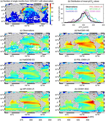
The carbon data were averaged into monthly means over 4°×4° regular bins. The 4°×4° grid size was selected because it gives a reasonable temporal coverage and yet is still able to represent the large-scale spatial patterns of variability, while reducing the impact of mesoscale variability. This is particularly useful when comparing the spatial variability from the observations with those from relatively coarse models. Figure 1a shows the number of months with at least one measurement in each 4°×4° box over the time period of our study. The northern hemisphere is generally well sampled with best coverage in the western North Pacific, in the North Atlantic between the Caribbean and the United Kingdom (Schuster and Watson, 2007), and between Denmark and Greenland (Olsen et al., 2008). The observation density is sparse throughout most of the Indian Ocean and South Pacific and South Atlantic Oceans. The Indian Ocean is strongly under-sampled because only a few observations have been collected in the last decade. In the Southern Ocean, the best coverage is across the Drake Passage (Takahashi et al., 2011).

Fig. 1 (a) Number of months with at least one observation between 1970 and 2011 based on data regridded onto a 4°×4° grid (the potential maximum is 504 months; white colour represents no data). (b) Distribution of long-term mean (1991–2011) pCO₂ values as number of grid cells per 2 µatm interval from the observations and all models. (c–h) Maps of long-term (1991–2011) mean pCO₂ from observations and models.

2.2. Model simulations

We have used output from five state-of-the-art Earth system model (ESMs) simulations. The five models are the Norwegian ‘NorESM1-ME’, the Hadley Centre's ‘HadGEM2-ES’, the Institut Pierre Simon Laplace's ‘IPSL-CM5A-LR’, the Max Planck Institute for Meteorology's ‘MPI-ESM-LR’, and the Community Earth system model ‘CESM1-BGC’ developed in the United States under the coordination of the National Center for Atmospheric Research (NCAR). All five models simulate the surface ocean carbon chemistry and ecosystem dynamics prognostically. Brief descriptions and references for all models are available in the Supplementary file. Historical and future scenario simulations have been made using these models as part of the Coupled Model Intercomparison Project phase 5 (CMIP5, Taylor et al., 2012). The model simulations also contribute to the Fifth Assessment Report of the Intergovernmental Panel on Climate Change (IPCC-AR5). The capacity of these models to simulate the ocean carbon sink and biogeochemical change over the 21st century has been documented (e.g. Bopp et al., 2013; Jones et al., 2013). We note that although the ESMs simulate their own internal climate variability, which differs from that recorded in the observational data sets, the long-term trend in surface pCO₂, to the first order, should follow the atmospheric CO₂ growth rate.

Four of the five models chosen here are from host institutions and partners of the ongoing European Union project CARBOCHANGE, which aims to explore the changes in ocean carbon uptake and emissions in a changing climate. The CESM1-BGC model was added due to its close connection to the NorESM1-ME model (e.g. they both use similar atmospheric general circulation models). All model outputs were downloaded from the CMIP5 repository (http://pcmdi9.llnl.gov). Here, for consistency with the observational period, we analyse the same 1970–2011 period. The model data were taken from the ‘historical’ simulation up to year 2005, combined with the ‘RCP8.5′ (Representative Concentration Pathways) future scenario for the years 2006–2011. In addition to the contemporary period, we also analyse the model trends over the last 40 yr of the 21st century (i.e. 2061–2100) under the RCP8.5 scenario. In the RCP8.5, the atmospheric CO₂ increases to 936 ppm in year 2100 and, along with other forcings, represents an additional radiative forcing of approximately 8.5 W m⁻² (Moss et al., 2010). We note that the current emissions or atmospheric pCO₂ trends follow the RCP8.5 scenario or are even somewhat higher (Peters et al., 2012).

In both historical and RCP8.5 simulations, all models use the same prescribed atmospheric CO₂ concentrations, aerosols, and other greenhouse gases (e.g. CFCs and CH₄) as outlined in Taylor et al. (2012). We derived the monthly surface ocean pCO₂ model fields from the prognostic monthly ALK, DIC, SST, and SSS fields using the carbon chemistry formulation as described in the previous subsection. This allows a more consistent interpretation of the model output when we later investigate the effects of the individual controlling factors (i.e. SST, SSS, DIC, and ALK) for the surface pCO₂ trend.

To ensure that the model outputs were consistent with the observations, we also interpolated them onto the same 4°×4° regular grid using uniform weighting for all data within each grid cell. This interpolation is also useful from the model point of view as each model usually has a unique grid configuration, so it simplifies the model–model and model-data analysis. The thickness of the upper model layer is 10 m, except for the NorESM1-ME (5 m).

2.3. Regional trend computation

Applying the observations and model data, we calculated the pCO₂ trend in 14 large-scale oceanographic regions. The 14 regions were defined by dividing the Atlantic and Pacific Oceans into subpolar north, subtropical north, equatorial, and subtropical southern parts. The Indian Ocean was divided in the same manner but without a subpolar north region. The remaining regions are the Arctic and the high-latitude Southern Ocean. In addition, the subpolar North Pacific was further divided into a western and an eastern part due to their contrasting biogeophysical characteristics (e.g. Takahashi et al., 2006). This regional division is similar to that used by Lenton et al. (2012). Table 1 lists the 14 regions together with their boundaries and abbreviations.

Table 1. Definition of the 14 regions used to assess the large-scale trends in surface pCO₂

Acronym	Region	Boundaries
ARC	Arctic Ocean	North of 62°N
WSPNP	Western subpolar North Pacific	40°N–62°N, west of 180°E
ESPNP	Eastern subpolar North Pacific	40°N–62°N, east of 180°E
STNP	Subtropical North Pacific	10°N–40°N
EP	Equatorial Pacific	10°S–10°N
STSP	Subtropical South Pacific	45°S–10°S
SPNA	Subpolar North Atlantic	40°N–62°N
STNA	Subtropical North Atlantic	10°N–40°N
EA	Equatorial Atlantic	10°S–10°N
STSA	Subtropical South Atlantic	45°S–10°S
NI	North Indian	North of 10°N
EI	Equatorial Indian	10°S–10°N
STSI	Subtropical South Indian	45°S–10°S
SOC	High-latitude Southern Ocean	South of 45°S

To compute the regional pCO₂ trends for the 1970–2011 period, we perform the following steps on both the observational and model data:

1. Remove regional-aliasing by subtracting the local long-term mean (i.e. 1971–2011) pCO₂ from the monthly mean pCO₂ field in each 4°×4° cell.

2. Average (area-weighted) the monthly values within the 14 regions. Thus, for a full coverage in each region, there are 504 (12 months times 42 yr) monthly pCO₂ values.

3. Deseasonalize the resulting monthly mean pCO₂ time-series in each region by subtracting out the long-term mean of each month (January, February, etc.).

4. Apply a linear regression to calculate the regional pCO₂ trend.

The above steps are applied to generate regional long-term pCO₂ trends from observations and model output. Step 1 is necessary to avoid spatial bias in the regionally averaged trend. For example, if within one region (of the 14) there are more data in the earlier period from grid boxes with climatologically low pCO₂ and more data at the end of the period from grid boxes with high pCO₂, the computed regional trend could be biased towards higher trend when step 1 is not applied.

2.4. Decomposition of pCO₂ trend

Here, we assume that the actual pCO₂ trend (‘dpCO ₂ /dt’) is approximately equal to the sum of four decomposed trends (‘’), where x is SST, SSS, DIC, or ALK:1

and2 3 4 5 6

where f represents the set of thermodynamic equations that relates the inorganic carbon species. The actual local (4°×4°) monthly pCO₂ in eq. (2) is computed by applying monthly varying SST, SSS, DIC, and ALK. Each of the in eqs. (3)–(6) represents the monthly pCO₂ field computed by applying a monthly varying x field, while the other three fields were kept at their long-term local average values (e.g. 1970–2011). Thus, is an estimate of the monthly local pCO₂ field as a result of changing SST only. The local long-term trends of the left-hand side terms in eqs. (2)–(6) (e.g. dpCO ₂ /dt or ) are computed by applying steps 3 and 4, as described in the previous Subsection 2.3. Therefore, the is an indicator for the pCO₂ trend resulting from the long-term change in SST. The same approach was applied for the other three parameters (i.e. SSS, DIC, and ALK).

Our pCO₂ trend decomposition is useful to identify the main drivers regulating the trend, and provides insight on the controlling mechanisms acting in different regions. To do this requires good temporal coverage of SST, SSS, DIC, and ALK, which is generally lacking in the observational data set. For this reason, the decomposition was only applied to the model data and the available long-term observations at BATS and HOT stations. In case only underway pCO₂ observations were available at these locations, ALK values were filled with those computed using Lee et al. (2006). Missing DIC values were then calculated from these and the observed pCO₂.

3. Results

A comparison of time-averaged surface pCO₂ from the observations and from each of the models over the years 1991–2011 is shown in Fig. 1c–h. The long-term mean maps highlight the main large-scale structures of the surface ocean pCO₂ as observed and as simulated by the models. The observed large-scale patterns of pCO₂ are well reproduced by the models with maximum values found in the equatorial Pacific and minimum values in subpolar North Atlantic, western North Pacific, and parts of the Southern Ocean. Nevertheless, there are some discrepancies in the magnitude of pCO₂. For example, in the eastern equatorial Pacific where the pCO₂ maximum is associated with upwelling of old DIC-rich water masses, the pCO₂ is considerably underestimated by the HadGEM2-ES and overestimated by the CESM1-BGC. The models generally overestimate the pCO₂ in the North Atlantic subtropical gyre and parts of the Southern Ocean.

Figure 1b shows the distribution of the mean pCO₂ values over the grid cells (i.e. number of grid cells per pCO₂ interval) from the data and models in the form of a histogram plot. We note that the histograms would, by construction, give more weight to the high latitudes with low pCO₂ values (i.e. each latitude band has the same number of grid boxes, despite the fact that the grid cells in polar regions have smaller areas than those in low latitude regions). For the 1991–2011 period, the observations and models show a distribution ranging from 250 to 450 µatm with a peak near 350 µatm. The models’ distributions are comparable with those of the observations, with a few exceptions. There is a small peak at 300 µatm in the HadGEM2-ES and IPSL-CM5A-LR distributions, related to the pCO₂ in the Arctic. The area of high pCO₂ waters in the tropical region of the NorESM1-ME is considerably larger than the data and other models, hence the pCO₂ distribution from this model is skewed towards high values.

3.1. Contemporary pCO₂ trends

For the contemporary period (1970–2011), the atmospheric CO₂ trend recorded at the Mauna Loa station is 1.61 ppm yr⁻¹ (http://www.esrl.noaa.gov/gmd/ccgg/trends/). This is representative of the global atmospheric CO₂ trend, which has a regional variability of approximately ±0.1 ppm yr⁻¹ (GLOBALVIEW-CO₂, 2012). The trend of atmospheric CO₂ partial pressure prescribed as the boundary condition in the CMIP5 model simulations is the same for the analysed period. Note that the surface ocean pCO₂ trends reported here are in µatm yr⁻¹ units and for comparison with atmospheric CO₂ trend, we assume that there are insignificant differences between µatm yr⁻¹ and ppm yr⁻¹ units.

Following steps 1–3 described in Subsection 2.3, we generated time-series of monthly pCO₂ anomalies from the observations and from each model for the 14 ocean regions, as shown in Fig. 2. We note that the observed values (black markers) in Fig. 2 are, in some regions, slightly lower than the model values. This is because the local correction (step 1 in Subsection 2.3) was computed over the whole 1970–2011 period. Hence, the anomalies of the observations are zero around the period with most data. In most regions, a pronounced increase in observational coverage from the 1990s onward is evident, and by the 2000s, the temporal observational coverage is very good in the northern hemisphere. This is also true for the Southern Ocean (south of 45°S), though the coverage here is confined to regions with high density of measurements (e.g. the Drake Passage) (Fig. 1a). The Indian Ocean and large parts of the Southern Ocean between 10°S–45°S remain under-sampled.

Fig. 2 Time-series of deseasonalized monthly pCO₂ anomalies from observations and five CMIP5 models for the 1970–2011 period in 14 ocean regions as defined in Table 1. The coloured numbers in each panel represent the standard deviation of the detrended model and observed time-series. Those inside the parenthesis represent standard deviation when the model data are subsampled following observational spatial and temporal coverage.

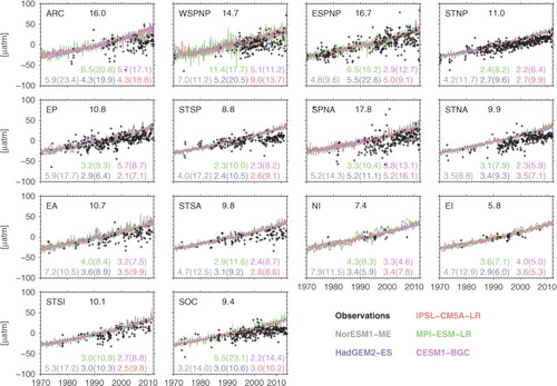
The standard deviation of the detrended observed and modelled time series, given in Fig. 2, shows that all models simulate weaker interannual variability than the observations. This is partly related to sparse observational coverage. When we subsampled the model output following the observational coverage, the standard deviation of the detrended time-series from each model increased and became more comparable to that of the observations. Thus, the interannual variability indicated by the observations may be biased towards those 4°×4° grid cells with the most ship tracks. In regions where there is good temporal coverage prior to the 1990s (e.g. ESPNP, STNP, and EP), the long-term increasing trends are more evident. All ESMs simulate a similar steady increase in surface pCO₂ of approximately 70 µatm between 1970 and 2011 in all regions.

3.1.1. Observed and simulated regional amplitude and variability

Here, we first present the regional pCO₂ trends derived from the observations and a comparison with estimates from earlier studies. Later, trends derived from model simulations are presented and compared with the observed trends. We applied a linear regression to the observational time-series data in Fig. 2 to produce the regional pCO₂ trends. These are shown as grey squares in Fig. 3 and the uncertainty ranges represent the 95% confidence intervals.

Fig. 3 Regional trends of surface pCO₂ computed from observations (grey squares). Blue circles (blue squares) represent multi-model-mean trend computed from the fully sampled model output (subsampled model output following observational coverage). All trends are for the 1970–2011 period. The uncertainty ranges for the observed trends represent the 95% confidence intervals whereas the uncertainty ranges for the model values represent ±1σ (one standard deviation) of the inter-model variations. The red-dashed line represents the atmospheric pCO₂ trend for the same period as observed at the Mauna Loa station (data were downloaded in February 2013). The abbreviations for the regions on the x-axis are defined in Table 1 and the total number of months with observation (of potentially 504 months) available for each region is given on the top x-axis.

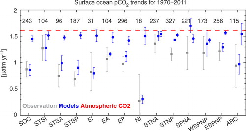
The observed trends are lower than the atmospheric CO₂ growth rate of 1.61 µatm yr⁻¹ and significantly positive in all regions (except for NI), ranging from 0.69±0.14 µatm yr⁻¹ in STSP to 1.36±0.17 µatm yr⁻¹ in STNA. The observed trends in the equatorial and southern hemisphere ocean are generally lower than those in the northern hemisphere. In SPNA, WSPNP, and ARC the poor data coverage in the 1970s and 1980s explains the large uncertainty range. However, in nearly all of the Pacific regions (ESPNP, STNP, EP, and STSP), the uncertainty ranges are smaller and consistent with the better data coverage in the earlier periods. Due to very limited data coverage in the NI and EI with only 18 and 31 monthly observations, respectively, the computed trend is unlikely to be representative of the domain trend.

We compare our estimated trends with those from earlier studies in the Pacific basin as it has the highest data coverage and is one of the most well-studied regions with respect to the surface pCO₂ trend. In STNP where 327 monthly measurements are available, our trend estimate of 1.16±0.13 µatmyr⁻¹ is comparable with the mean trend of 1.24 µatmyr⁻¹ for the 1970–2004 period determined by Takahashi et al. (2006). In the WSPNP, our observation-based trend estimate of 1.18±0.31 µatm yr⁻¹ is well within the range reported by Lenton et al. (2012) of 1.6±1.7 ppm yr⁻¹ for the 1993–2007 period. In their study, Takahashi et al. (2006) estimated pCO₂ trends within 10°×10° grid bins over the North Pacific between 1970 and 2004. They showed that in WSPNP, the gridded trends vary considerably, from −1.42±0.42 to 1.30±3.2 µatm yr⁻¹. In the equatorial Pacific region (10°S–10°N), our observed pCO₂ trend of 0.98±0.14 µatm yr⁻¹ is in the lower range of the estimate by Feely et al. (2006) of 1.32±0.56 and 1.16±0.27 µatm yr⁻¹ for the western Pacific warm pool and Niño 3.4 regions, respectively, for the 1974–2004 period.

Next, we computed the regional pCO₂ growth rates over the same period using model outputs. These are shown as the blue circles in Fig. 3. The uncertainty ranges represent one standard deviation of the inter-model spread. Compared to the trend derived from observations, the model-derived trends are always higher and very close to the atmospheric CO₂ trend (within 0.2 µatm yr⁻¹ of the atmospheric CO₂ trend). The simulated pCO₂ trends are also very consistent among models, indicated by the small inter-model spreads (±1 σ), except in the ARC and NI regions.

In order to examine how sensitive the model trends are to the sampling coverage, we subsampled the model output according to the spatial and temporal coverage of the observational data set. Afterwards, we repeated the four steps described in Subsection 2.3 to arrive with a second set of (i.e. subsampled) model-derived regional trends. The subsampled model trends are shown as blue squares in Fig. 3.

Figure 3 shows that, aside from SPNA, the subsampled model trends are always lower than the fully sampled model trends. In nearly all equatorial and southern hemisphere domains, the subsampled model trends do not overlap with the fully sampled trends. In all of these regions, the subsampled trends are also much closer to the observation-derived trends. Specifically, excluding STNP and SPNA, the subsampled trends are now within or overlap with the trends derived from the observations. This suggests that the model-mean performance compares favourably with the data and increases our confidence in the model results.

There are several factors that could contribute to the lower subsampled than fully sampled model trends. The first is related to insufficient spatial coverage in a specific ocean basin. This can be seen in the regions SOC, EI, and NI. In SOC, despite a reasonable temporal sampling (as seen in Fig. 2), the measurements are confined to a relatively small region in the proximity of the Drake Passage (see Fig. 1a) relative to the much larger and biogeochemically diverse SOC region (Marinov et al., 2006; Lovenduski et al., 2008). In the poorly covered EI and NI, the subsampled model trends also deviate significantly from the fully sampled trends. The former is now within the large range of trends derived from observations. Spatial bias in the observational coverage can also be seen in the STSA and STSP (Fig. 1a), where the data density is higher near the western boundary of subtropical gyres. In these two regions, the model simulations show that the pCO₂ trends are stronger in the centre and eastern part of both gyres (e.g. see also Fig. 5).

The second factor could be related to a bias in the temporal sampling (i.e. few measurements in the 1970s and 1980s). To examine whether this is the case, we recomputed the fully sampled model trends, but using different starting years (i.e. 1970, 1971 … 1990) and the same ending year of 2011. Our results show that in nearly all regions, the recomputed trends increase (rather than decrease) when the starting date is moved forward (see Supplementary file). This is consistent with the fact that the atmospheric CO₂ is growing at a faster rate in the later part of the 1970–2011 period. We therefore suggest that the temporal coverage of the observations, which is more dense towards the later period, is not the main reason for the lower observation-based and subsampled model pCO₂ trends.

This exercise highlights that good coverage in time and space is needed in order to determine robust regional long-term pCO₂ trends. With the exception of a few regions, sufficient coverage does not yet exist. For example, in the relatively small area STNA, the subsampled trend does not deviate far from the fully sampled trends. Here, the spatial coverage is more uniform and there are 237 months with observations; pCO₂ trends determined from the current observational coverage may be representative of the larger scale basin wide trends.

3.1.2 Regional drivers for pCO₂ trends

In this Subsection, we present the local (within 4°×4° grid boxes) pCO₂ trends decomposed into four drivers by applying the method described in Subsection 2.4. Due to the limited availability of long-term measurements of high-quality surface DIC and ALK, we have selected only two locations, where the approach can be applied to the observed trend. These are BATS (Bates, 2012) located in the North Atlantic subtropical gyre (centred at 31°40′N, 64°10′W) and HOT located in the North Pacific subtropical gyre (centred at 22°45′N, 158°00′W).

Figure 4 shows the monthly pCO₂ anomalies from both the observations and each model together with the actual and decomposed pCO₂ trends at BATS and HOT stations for the 1970–2011 period. At BATS, the observed long-term increase of surface pCO₂ is generally well captured by all models. The observed dpCO ₂ /dt is 1.78±.28 µatm yr⁻¹, slightly higher than the model estimates, which ranges from 1.38 to 1.57 µatm yr⁻¹. Our estimated trend from observations is consistent with the trend reported by Bates et al. (2012) of 1.80±0.09 µatm yr⁻¹ for the 1983–2011 period. The models generally agree with the observations in identifying the dominant combination of drivers (SST, SSS, DIC, or ALK) that explains the overall pCO₂ trend. Both model and observations indicate that the increase in DIC is the main driver of the pCO₂ trend. Increases in SST and ALK lead to small positive () and negative () trends, respectively. As expected, the direct impact of SSS on the long-term pCO₂ trend () is very small. Our estimates are consistent with an earlier study, which finds a significant increase in surface DIC accompanied by a small ALK increase over the last three decades. This would lead to increase and decrease of the surface pCO₂ trend by +122% and −33%, respectively (Bates et al., 2012). When considering their uncertainty ranges, the sum of all four trend components () is indistinguishable from the actual trend (dpCO ₂/dt) in three of five models and in the observations. This suggests that our decomposition method gives a reasonable approximation of the actual changes due to each driver.

Fig. 4 Deseasonalized monthly anomalies of pCO₂ fields from observations and models for (a) BATS and (c) HOT. (b,d) Decomposed annual pCO₂ growth rate for the 1970–2011 period at (b) BATS and (d) HOT from observations and models. Shown here are pCO₂ trends associated with long-term variations of SST ( /dt), SSS ( /dt), DIC ( /dt), and ALK ( /dt). The sum of these four components (dpCO /dt) is also shown as a comparison with the actual pCO₂ trends (dpCO ₂/dt). The horizontal dashed lines represent the atmospheric pCO₂ trend for the same period and the vertical lines represent the uncertainty range.

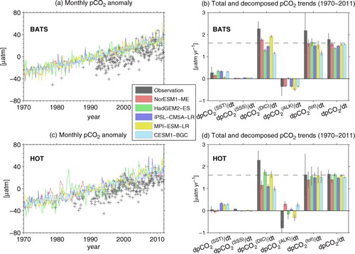
At HOT, the observations also indicate similar long-term increase of the surface pCO₂ as the models. Similar to BATS, both models and observations suggest that the long-term change in DIC mostly explains the overall pCO₂ trends. The observations also indicate weak negative , and weak and . A similar pattern is also simulated by the models, although only two models capture the weak negative . For HOT, the sum of all four terms from all models is also very close to the observed trend (). The model-data comparisons at BATS and HOT are useful to illustrate that the models are in general capable of identifying the main driver explaining the pCO₂ trends at these different locations over the studied period.

Next, we computed the decomposed pCO₂ for all grid boxes using only models. Figure 5 shows maps of the model mean of the decomposed trends together with the total and actual pCO₂ trends for the 1970–2011 period. For this period, Fig. 5 reflects that a surface warming is simulated in nearly all regions, with the exception of small areas in the North Atlantic and Southern Ocean. The surface warming is translated into positive in the order of 0.2–0.3 µatm yr⁻¹. The long-term changes in SSS have almost negligible influence on surface pCO₂. For most of the world ocean, with the exception of the Arctic, the model mean shows that the trend due to increasing surface DIC () to the first order explains the magnitude and spatial pattern of the total trends, . The component is strongest in the subtropical oceans in both hemispheres as well as over most of the Southern Ocean.

Fig. 5 Maps of model mean of (a–d) decomposed pCO₂ trends due to change in SST, SSS, DIC, and ALK together with (e) sum of all decomposed trends and (f) actual pCO₂ trend for the 1970–2011 period. Contour lines at ‘1.61’ in (e–f) represent the growth rate of atmospheric pCO₂ for the same period. The stippling in (f) indicates regions where all five models agree whether the actual pCO₂ trend is stronger or weaker than the atmospheric pCO₂ trend.

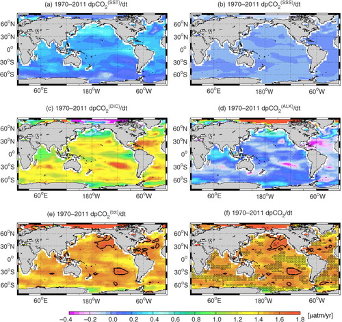
The trend associated with ALK () is generally weak and exhibits a similar spatial pattern but in the opposite sign from that of . Surface ALK increases (i.e. negative ) are shown by the model mean in the subtropical North and South Atlantic Oceans as well as in the subtropical South Pacific. Here, increases in ALK are associated with the changes in freshwater fluxes, through increased salinification (i.e. higher evaporation than precipitation). In the Arctic, the change (decrease) in surface ALK is the main driver for the positive surface pCO₂ trend.

Despite the dominant role of the DIC increase, changes in SST and ALK play a considerable role in several regions. In the subtropical South Pacific and subtropical North Atlantic, large is slightly alleviated by the negative . In the eastern equatorial and subpolar North Pacific, relatively weak is enhanced by positive . Relatively strong in these two regions could also explain the weak , since warming leads to increasing stratification and low CO₂ solubility. These mechanisms lead to a reduced upwelling of deep water with low anthropogenic carbon concentrations to the surface and weaker CO₂ uptake from the atmosphere, hence low . Figure 5 also shows that the accumulated decomposed trends () resemble the actual trend (dpCO ₂ /dt), which is very close to the atmospheric CO₂ trend of 1.61 ppm yr⁻¹ for the same period. The model mean also shows that the trends in the high-latitude Southern Ocean, eastern equatorial Pacific, and subpolar North Atlantic are clearly weaker than the atmospheric trend.

To quantify the long-term contributions of the different drivers in the 14 ocean regions defined earlier, we computed area-weighted averages for each term in Fig. 5 and summarize them in Table 2. Included in Table 2 are the relative contributions (%) from each term to the total trend. The surface warming leads to positive in all regions. The is largest in the subpolar North Pacific, where warming accounts for approximately one-quarter of the total trends in WSPNP and ESPNP. The temperature-related trend is lowest in the SOC, accounting for only 9% of the overall trend. For the contemporary period, in all regions except for the Arctic, the steady increase of surface DIC is mainly responsible and explains at least 51% of the total pCO₂ trend. In all oceans in the subtropical regions (10°N–40°N and 45°S–10°S), surface DIC accumulation accounts for at least 85% of the total trend. As stated earlier, changes in surface ALK contribute negatively to the overall trends in the STSP, STNA, and STSA. In the STNA, negative approximately offsets the positive due to warming. Consequently, the increase in pCO₂ in STNA can be attributed largely to the increase in surface DIC (i.e. 94%, as shown in Table 2). In the Arctic, the uncertainty ranges for and are both large, suggesting that the inter-model spread is large.

Table 2. Region-averaged pCO₂ trends for the 1970–2011 period associated with changes in SST ( /dt), SSS ( /dt), DIC ( /dt), and ALK ( /dt) as computed from the mean of all five models

Region	/dt	/dt	/dt	/dt	/dt	dpCO 2/dt
ARC	0.18±.08(9)	−0.05±.03(−3)	0.46±.74(24)	1.35±.91(70)	1.94±.36	1.54±.21
WSPNP	0.37±.14(26)	−0.01±.02(−1)	0.87±.31(61)	0.19±.29(14)	1.42±.04	1.43±.04
ESPNP	0.35±.19(22)	−0.03±.03(−2)	0.80±.36(51)	0.45±.37(29)	1.58±.04	1.57±.03
STNP	0.22±.07(15)	−0.00±.01(0)	1.30±.15(85)	0.01±.12(1)	1.53±.04	1.52±.04
EP	0.26±.07(18)	−0.01±.02(−1)	1.12±.23(76)	0.08±.19(5)	1.44±.09	1.42±.08
STSP	0.19±.05(12)	0.00±.01(0)	1.36±.11(89)	−0.02±.08(−2)	1.53±.05	1.52±.06
SPNA	0.21±.12(14)	−0.01±.03(−1)	1.14±.17(74)	0.19±.35(12)	1.53±.15	1.46±.07
STNA	0.26±.10(17)	0.03±.01(2)	1.46±.17(94)	−0.20±.08(−13)	1.55±.05	1.54±.05
EA	0.28±.09(18)	0.00±.02(0)	1.25±.21(78)	0.06±.28(4)	1.60±.15	1.48±.10
STSA	0.22±.07(15)	0.01±.01(1)	1.33±.11(89)	−0.08±.11(−5)	1.49±.05	1.48±.05
NI	0.26±.11(17)	−0.02±.01(−2)	1.10±.17(73)	0.18±.19(12)	1.52±.14	1.51±.15
EI	0.26±.08(17)	−0.03±.01(−2)	1.00±.19(66)	0.29±.16(19)	1.52±.10	1.51±.11
STSI	0.21±.04(14)	0.00±.01(0)	1.32±.16(87)	−0.01±.10(−1)	1.52±.07	1.51±.07
SOC	0.12±.06(9)	0.00±.01(0)	1.25±.23(87)	0.07±.17(5)	1.44±.05	1.45±.05

/dt is the sum of all trend components, and therefore is slightly different from dpCO ₂/dt (blue circles in Fig. 3) computed from the actual pCO₂ values. The uncertainty ranges represent 1σ of the inter-model spread. Unit is µatm yr⁻¹. The numbers within parentheses represent the relative contribution of each driver to the total trend (%). The atmospheric pCO₂ trend for the same period is 1.61 ppm yr⁻¹.

To quantitatively estimate the regional influence of hydrological cycle changes or the dilution effect on the surface pCO₂ trends in the models, we computed the pCO₂ trends associated with the SSS -normalized surface DIC () and ALK (). We compute nDIC and nALK by normalizing the monthly gridded DIC and ALK from each model to long-term mean local surface SSS, thereby removing the long-term changes of surface freshwater fluxes. The SSS -normalized trends are computed with the same method as described in Section 2.4 by replacing DIC and ALK with nDIC and nALK, respectively. Here, we assume that freshwater does not carry carbon or ALK, which is reasonable for open ocean regions, where freshwater fluxes are dominated by precipitation and evaporation processes. We note that this is not the case in the Arctic, where riverine runoff can play a bigger role (e.g. in Arctic river runoff, DIC concentration can be as large as 1700 µmol kg⁻¹, Anderson et al., 1998). Not all models used here include DIC and ALK in the riverine influx (see also Supplementary file).

Figure 6 shows maps of and computed from the model mean over the period 1970–2011. Additionally, we also show the total contribution of freshwater-induced DIC and ALK changes on the surface pCO₂ trends (i.e. =+−−). The area-weighted averages of each term for the 14 ocean regions are summarized in Table 3.

Fig. 6 Maps of model mean of decomposed pCO₂ trends due to change in salinity-normalized (a) DIC and (b) ALK for the 1970–2011 period. The total contribution of surface freshwater flux on the DIC- and ALK-associated pCO₂ trend (=+−−) is shown in panel (c).

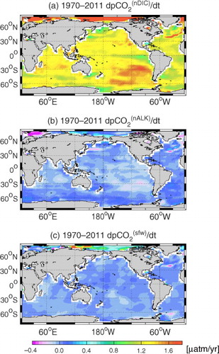
Table 3. Region-averaged pCO₂ trends for the 1970–2011 period associated with changes in salinity-normalized DIC ( /dt) and ALK ( /dt) as computed from the mean of all five models

Region	/dt	/dt	/dt
ARC	1.62±.12	0.02±.11	0.18±.44
WSPNP	1.11±.23	−0.01±.11	−0.03±.05
ESPNP	1.23±.21	0.04±.10	−0.02±.04
STNP	1.32±.10	−0.02±.05	−0.00±.01
EP	1.24±.17	−0.05±.05	0.01±.03
STSP	1.38±.06	−0.05±.04	0.00±.01
SPNA	1.34±.25	−0.01±.08	0.00±.09
STNA	1.21±.24	0.02±.09	0.02±.01
EA	1.19±.21	0.02±.08	0.10±.18
STSA	1.17±.14	0.06±.07	0.02±.01
NI	1.49±.49	−0.04±.07	−0.17±.38
EI	1.33±.09	−0.02±.10	−0.02±.02
STSI	1.36±.13	−0.04±.05	−0.02±.04
SOC	1.28±.14	0.04±.09	−0.01±.01

/dt represents the surface fresh water flux contribution (dilution of DIC and ALK) to the total pCO₂ trend ( /dt= /dt + /dt− /dt− /dt). Therefore, negative (positive) dpCO /dt indicates that a change in freshwater flux reduces (increases) the overall pCO₂ trend. The uncertainty ranges represent 1 σ of the inter-model spread. Unit is µatm yr⁻¹.

As shown in Fig. 6 and Table 3, the field is positive everywhere. This is associated with an increase in surface DIC concentration as a result of anthropogenic carbon invasion. The map of approximately resembles the map of shown in Fig. 5, with only a few exceptions. In the equatorial Indian Ocean, subpolar North Pacific, Arctic Ocean, and parts of the Southern Ocean, an increase in freshwater input is simulated, shown by higher than . This is related to the increase in precipitation and ice-melt in the Arctic Ocean. In contrast, an increase in evaporation is detected in most parts of the Atlantic Ocean (i.e. >).

Table 3 and Fig. 6 show that in nearly all regions, the is very close to zero. This suggests that the regional pattern of shown in Fig. 5d must be related to the long-term changes in freshwater fluxes, as described in the previous paragraph. The total contribution of the dilution effect () is also very close to zero everywhere. This is expected since the dilution effect acting on DIC approximately offsets the dilution effect on ALK, when calculating the surface pCO₂. Data in Fig. 5b and 6c are both close to zero and nearly indistinguishable. This suggests that the effect of pCO₂ changes associated with freshwater flux on the carbonate system is equally small relative to the combined dilution effects on DIC and ALK. This is true for most of the ocean regions, except for the Arctic, as shown in Table 2 column 3 and Table 3 column 3.

3.2. Future pCO₂ trend

In this subsection, we used the model output to assess the actual long-term pCO₂ trend and its drivers over the last 40-yr (2061–2100) of the 21st century under the RCP8.5 scenario. As done for the contemporary period, we decomposed the total pCO₂ trend into four driving terms from SST, SSS, DIC, and ALK. Figure 7 shows maps of the model-mean decomposed trends together with the total and the actual pCO₂ trends. The regionally averaged trends of each driver, and its contribution to the total trend, are provided in Table 4. We also computed maps and regionally averaged pCO₂ trends associated with normalized DIC and ALK (Fig. 8 and Table 5). Changes in SSS have negligible contributions to the overall pCO₂ trend in all regions relative to the other three terms, and thus are not discussed further here. In the ARC region, the simulated trends vary significantly, as shown by the large inter-model spread in Table and 5 .

Fig. 7 Maps of model mean of (a–d) decomposed pCO₂ trends due to change in SST, SSS, DIC, and ALK together with (e) sum of all decomposed trends and (f) actual pCO₂ trend for the 2061–2100 period of the RCP8.5 scenario. Contour lines at ‘8.41’ in (e–f) represent the growth rate of atmospheric pCO₂ for the same period. The stippling in (f) indicates regions where all five models agree whether the actual pCO₂ trend is stronger or weaker than the atmospheric pCO₂ trend.

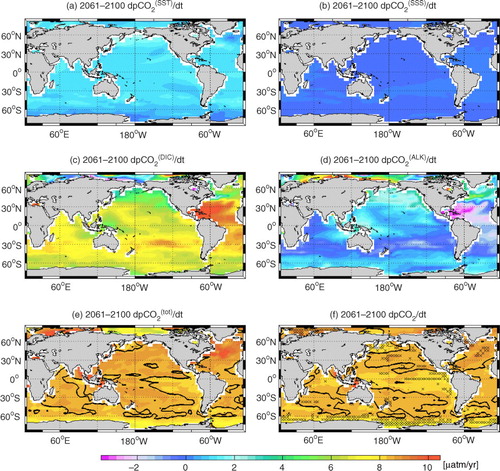
Fig. 8 Maps of model mean of decomposed pCO₂ trends due to change in salinity-normalized (a) DIC and (b) ALK for the 2061–2100 period of the RCP8.5 scenario. The total contribution of surface freshwater flux on the DIC- and ALK-associated pCO₂ trend is shown in panel (c).

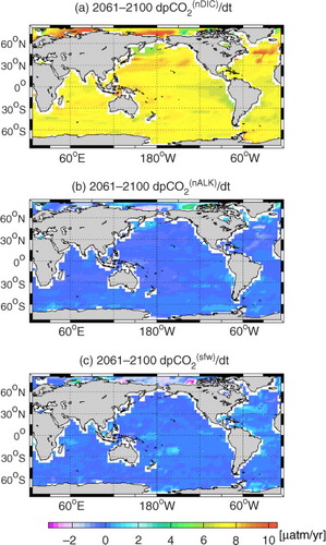
Table 4. Region-averaged pCO₂ trends for the 2061–2100 period of the RCP8.5 scenario associated with changes in SST ( /dt), SSS (dpCO /dt), DIC (dpCO /dt), and ALK (dpCO /dt) as computed from the mean of all five models

Region	dpCO /dt	dpCO /dt	dpCO /dt	dpCO /dt	dpCO /dt	dpCO 2/dt
ARC	0.98±.45(12)	−0.17±.16(−2)	2.06±2.99(25)	5.37±3.50(65)	8.23±.58	8.62±.23
WSPNP	1.49±.27(18)	−0.12±.06(−1)	4.32±.81(52)	2.64±.92(32)	8.33±.35	8.40±.15
ESPNP	1.43±.33(17)	−0.11±.04(−1)	4.78±.97(57)	2.23±.70(27)	8.33±.21	8.46±.13
STNP	1.09±.22(13)	−0.09±.08(−1)	6.30±.80(74)	1.16±.69(14)	8.45±.11	8.39±.21
EP	1.19±.33(14)	−0.08±.04(−1)	6.38±1.04(76)	0.85±.62(10)	8.34±.38	8.19±.35
STSP	1.08±.18(13)	0.01±.01(0)	7.51±.49(89)	−0.21±.36(−2)	8.39±.18	8.35±.22
SPNA	1.02±.41(12)	−0.12±.14(−1)	5.40±1.81(61)	2.60±2.04(29)	8.90±.30	8.62±.04
STNA	1.08±.33(13)	0.15±.02(2)	9.30±.57(109)	−1.97±.37(−23)	8.55±.32	8.42±.35
EA	1.22±.34(14)	0.09±.06(1)	8.59±.72(97)	−1.08±.72(−12)	8.83±.41	8.33±.38
STSA	1.14±.28(14)	0.07±.05(1)	8.16±.57(97)	−0.98±.64(−12)	8.40±.16	8.32±.22
NI	1.27±.18(15)	−0.01±.11(0)	6.78±1.60(80)	0.44±1.98(5)	8.49±.34	8.14±.21
EI	1.21±.23(14)	−0.01±.03(0)	7.00±.70(83)	0.24±.72(3)	8.43±.30	8.30±.28
STSI	1.07±.16(13)	−0.03±.02(0)	7.27±.52(86)	0.11±.43(1)	8.42±.14	8.39±.23
SOC	0.85±.20(10)	−0.03±.01(0)	6.58±.57(80)	0.83±.36(10)	8.24±.15	8.29±.17

dpCO /dt is the sum of all trend components, and therefore is slightly different from dpCO ₂/dt computed from the actual pCO₂ values. The uncertainty ranges represent 1σ of the inter-model spread. Unit is μatm yr⁻¹. The numbers within parentheses represent the relative contribution of each driver to the total trend (%). The atmospheric pCO₂ trend for the same period is 8.41 ppm yr⁻¹.

Table 5. Region-averaged pCO₂ trends for the 2061–2100 period of the RCP8.5 scenario associated with changes in salinity-normalized DIC (dpCO /dt) and ALK (dpCO /dt) as computed from the mean of all five models

Region	dpCO /dt	dpCO /dt	dpCO /dt
ARC	7.99±2.59	−0.01±1.97	−0.56±.56
WSPNP	6.82±1.04	0.13±.56	0.00±.21
ESPNP	7.38±.77	−0.23±.65	−0.13±.24
STNP	7.66±.50	−0.19±.45	−0.01±.08
EP	7.29±.81	−0.17±.39	0.11±.09
STSP	7.32±.49	−0.13±.34	0.11±.06
SPNA	7.98±1.12	−0.19±.95	0.21±.12
STNA	7.29±.65	−0.23±.48	0.26±.06
EA	7.01±1.25	−0.06±.65	0.56±.37
STSA	7.00±.72	0.02±.44	0.16±.08
NI	7.04±.97	−0.14±.68	0.32±.39
EI	7.19±.69	−0.07±.46	0.11±.16
STSI	7.70±.68	−0.34±.46	0.02±.10
SOC	7.34±.42	0.07±.33	−0.01±.07

dpCO /dt represents the surface fresh water flux contribution (dilution of DIC and ALK) to the total pCO₂ trend. Therefore, negative (positive) dpCO /dt indicates that change in freshwater flux reduces (increases) the overall pCO₂ trend. The uncertainty ranges represent 1σ of the inter-model spread. Unit is μatm yr⁻¹.

In all regions, the magnitude of increases everywhere relative to the contemporary period (Fig. 7a vs. Fig. 5a). Positive in all regions indicates that future climate warming will continue to contribute to the surface ocean pCO₂ growth rate, and can act as a positive feedback to climate change. The model increase of SST is lowest in the SOC, yielding 0.027°C yr⁻¹ SST growth rate for the period 2061–2100. It also shows the weakest change relative to the contemporary period. The in the SOC is smaller relative to the other regions (see also Table 4). Between 2061 and 2100, the majority of the models simulate the largest mean SST increase in the WSPNP and the ESPNP, with model-mean SST trends of 0.052 and 0.049°C yr⁻¹, respectively. This large warming in the North Pacific is a robust feature, also found in larger CMIP5 model ensembles (Bopp et al., 2013). In both WSPNP and ESPNP, where temperature has a large influence on surface pCO₂ (e.g. Chierici et al., 2006; Takahashi et al., 2006), increases faster than in the other regions (Table 4).

The long-term increase in surface DIC is mostly responsible for the simulated surface pCO₂ trends in all regions, except in the Arctic, similar to the present-day trend. When regionally averaged, the increase in surface DIC alone would increase the pCO₂ by 97 to 109% in the equatorial and subtropical Atlantic (STSA, EA, and STNA, Table 4), but this effect is counteracted by the increase in ALK, which slightly decreases the pCO₂ by −12 to −23%. Similarly, the increase in surface DIC is shown to have the largest contribution in the Atlantic Ocean (between 40°S and 40°N) and in the subtropical South Pacific (Fig. 7c). In the subpolar North Pacific (WSPNP and ESPNP), the contribution of surface DIC to the pCO₂ trend is relatively weak. This can be explained by the relatively large simulated warming, which stratifies the upper ocean and thereby reduces the mixed layer depth and the upwelling of DIC-rich deep water. When the DIC field is SSS -normalized, the pCO₂ trends due to nDIC (Fig. 8a) show that the maximum increases in surface DIC occur in the subpolar North Atlantic, the western subtropical North Pacific, and part of the Arctic.

The differences between and are more pronounced in the future than in the contemporary period because the DIC concentration is higher in the later period. Additionally, the simulated changes in surface freshwater flux are more intense in the future with strong evaporation in the Atlantic (40°S and 40°N) and subtropical South Pacific. In contrast, all models simulate stronger surface freshening in the subpolar North Pacific, subpolar North Atlantic, western equatorial Pacific, and parts of the Southern Ocean over the last 40-yr of the 21st century than during the contemporary period (see Supplementary file). Reductions in freshwater input are projected for the low- and mid-latitude Atlantic and subtropical South Pacific. Using a different set of models, Stott et al. (2008) show similar changes in the surface freshwater flux patterns, which can be attributed to the changes in the Earth's hydrological cycle with larger atmospheric water transport from low to high latitudes. Figure 7 also suggests that the long-term impact of the evaporation and precipitation change on pCO₂ trend will mostly be due to the dilution effect rather than the SSS effect on carbonate chemistry.

As seen in the contemporary period, the small trends in (8b) imply that the changes in the surface freshwater flux are the main drivers of the (Fig. 7d). For example, large increases in evaporation in the subtropical North Atlantic during the 2061–2100 period explain the negative ALK-attributed pCO₂ trends. In contrast, positive trends in most of the Pacific are related to the dilution of ALK (lower ALK leads to higher pCO₂) due to higher precipitation in these regions. Despite the change in precipitation and evaporation patterns, the net effect of the surface freshwater flux on pCO₂ trend () is relatively small (see also Table 5) when compared to the effects of SST and DIC.

The long-term surface pCO₂ trends continue to closely track the prescribed atmospheric CO₂ trend, at 8.41 ppm yr⁻¹ for the 2061–2100 period (Fig. 7e and 7f). Considering the model spread and the uncertainty in the atmospheric trend (±0.1 ppm yr⁻¹), the regionally averaged model pCO₂ trends (dpCO ₂ /dt in Table 4) are mostly indistinguishable from the atmospheric CO₂ trend, except in SPNA. The SPNA has the largest model-mean pCO₂ trend of 8.62±0.4 µatm yr⁻¹ (Table 4). Here, the trend switches from being lower, during the contemporary period, to higher than the atmospheric pCO₂ trend. By contrast, in the eastern equatorial Pacific and high-latitude Southern Ocean, the model-mean pCO₂ trends are lower than the atmospheric trend.

3.3. Modelled air–sea CO₂ flux trends

In this subsection, we infer the evolution of air–sea CO₂ fluxes over the contemporary period and at the end of the 21st century under the RCP8.5 scenario by applying the pCO₂ trends derived earlier. Note that the interpretation of ocean carbon uptake from the pCO₂ trend in this study is based on the assumption that there is no significant long-term change in other drivers of air–sea CO₂ fluxes, such as the surface wind speed. Thus, weaker surface pCO₂ growth than the atmospheric one translates into an increase in ocean carbon uptake and vice versa.

For the contemporary period, Fig. 3 shows that all regional trends calculated from the observations are well below the atmospheric CO₂ growth rate. The CO₂ flux trends inferred from the model simulations indicate similarly increasing patterns. This suggests that a large portion of the world ocean has continued taking up anthropogenic CO₂ over the past four decades. The contour lines in Fig. 5e represent the atmospheric CO₂ trend at 1.61 µatm yr⁻¹. It illustrates that with the exception of the eastern North Pacific, eastern subtropical South Pacific and parts of the subtropical North Atlantic, the ocean CO₂ sink continues to increase.

Next, we explore the consistency of pCO₂ trends relative to the atmospheric CO₂ trends among the five models. In Fig. 5f, the stippling highlights regions where all five models have the same directional trend in surface pCO₂ relative to the atmospheric trend. In the eastern equatorial Pacific, eastern equatorial Atlantic, and some parts of the North Atlantic and Southern Ocean, all models simulate consistently that the carbon uptake by the ocean has continued to increase during the 1970–2011 period. In the equatorial Pacific (e.g. near the Niño 3.4 region), the model-mean estimate is comparable with Feely et al. (2006), where it was shown that surface pCO₂ increases at a rate lower than the atmospheric CO₂ by approximately −0.3 µatm yr⁻¹ for the 1974–2004 period. In the subpolar North Atlantic, the model-mean trend also compares favourably to the observational and modelling study by Schuster et al. (2013), which shows an increasing carbon sink over the period 1995–2009. In the high-latitude Southern Ocean (58°S–75°S), Lenton et al. (2013) also show an increase in ocean carbon uptake for the 1990–2009 period in an ensemble of ocean biogeochemical models.

For the 2061–2100 period, nearly half of the ocean regions have a pCO₂ trend that is higher than the atmospheric growth rate (Fig. 7e). Whereas the model-mean pCO₂ trend is lower relative to the atmospheric trend in approximately 90% of the surface ocean area in the 1970–2011 period, this number decreases to 57% over the last 40 yr of the 21st century. Only the eastern equatorial Pacific and high-latitude Southern Ocean are projected to have increasing CO₂ uptake, based on their weaker than atmospheric pCO₂ trends. This implies that by the end of the 21st century, the ocean CO₂ uptake rate is reduced in most regions. In the subpolar North Atlantic, where the model-mean pCO₂ trend is largest, the net air–sea CO₂ flux may even reverse.

The future model-mean pCO₂ trend is distinct from the trends over the contemporary period in several ways. First, the spatial variability in the pCO₂ trend over the future period (with a standard deviation of 0.41 µatm yr⁻¹; Fig. 7f) is more pronounced than over the present-day period (standard deviation=0.23 µatm yr⁻¹; Fig. 5f). Secondly, there are fewer regions where the models agree on whether or not the surface pCO₂ trend is faster than the atmospheric one, indicated by less regions with stippling in Fig. 7f. Still, there are several key regions where all models remain consistent with one another. For example, in the Labrador Sea, the northeast extension of the North Atlantic drift, and a small region in the central mid-latitude North Pacific (30°N), all models agree that the surface pCO₂ trends are higher than the atmospheric trend, indicating a strong likelihood that the ocean uptake rate will be considerably reduced by the end of the 21st century. In contrast, all models agree that, in the eastern equatorial Pacific and the high-latitude Southern Ocean, the CO₂ uptake rate will continue to increase.

To show the evolution of global mean surface pCO₂ and the ocean carbon sinks in response to the increasing atmospheric CO₂, we plotted time-series of globally averaged pCO₂ and globally integrated net CO₂ flux to the ocean. Figure 9a shows that all models simulate a global mean surface pCO₂ that follows the atmospheric CO₂ concentration closely between 1970 and 2100. Figure 9b illustrates the net annual CO₂ uptake by the ocean from 1970 to 2100. For the 1990–1999 period, the model-mean uptake is 1.89±0.19 PgC yr⁻¹, which is well within the latest estimate from Le Quéré et al. (2013) of 1.55–2.59 PgC yr⁻¹. The time-series shows that ocean uptake increases steadily from the present-day before it starts to stabilize, around year 2050, when the projected increase in atmospheric pCO₂ becomes more linear in the RCP8.5 scenario. By the end of the century, the model-mean net ocean uptake is 5.07±0.52 PgC yr⁻¹. This pattern of increasing and stabilizing CO₂ uptake is consistently shown in all models. It is also clear that the slowing down of regional ocean carbon sinks cannot be inferred from time-series of the global mean pCO₂ alone.

Fig. 9 Global mean time-series of (a) prescribed atmospheric and simulated ocean pCO₂, (b) simulated net air–sea CO₂ flux, and (c) simulated deviation of 40-yr surface ocean pCO₂ trend relative to the atmospheric pCO₂ trend. The pCO₂ trends are over 40-yr moving windows starting from 1970–2009 and ending with 2061–2100. Each grey line represents the simulation from one model.

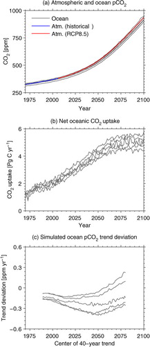
To see if the future stabilization of the ocean sink can be connected to the long-term surface pCO₂ trend, time-series of the global ocean 40-yr pCO₂ trends were computed for each model starting with the 1970–2009 and ending with the 2061–2100 period. The deviation of these trends from the atmospheric trends is plotted in Fig. 9c. It shows that globally, the ocean pCO₂ trends stay below the atmospheric trend for a few decades. All five models simulate trends, which remain weaker than the atmospheric CO₂ trend up to the 40-yr period centred around the year 2055. All models also simulate accelerating pCO₂ growth rates (faster relative to the atmospheric pCO₂ trend), roughly around year 2050, which coincides with the period when the ocean sink is projected to slow down before it finally stabilizes towards the end of the 21st century under RCP8.5. Beginning from the 40-yr period centred around 2075, two models simulate pCO₂ trends that are greater than the atmospheric trend. All models simulate similar long-term pCO₂ trends during the contemporary period but start to deviate in the future (Fig. 9c). Models with more similar initial trends tend to show a similar evolution for the projection periods.

4. Discussion

Surface ocean pCO₂ is a directly measurable biogeochemical parameter that can be used as an indicator of long-term climate change. It provides information on the ocean carbon sources and sinks as well as on any potential climate feedback due to changes in ocean biogeochemistry. In this study, we estimated the regional pCO₂ trends over the last four decades based on the latest data collection of directly and indirectly measured surface pCO₂. Model outputs were also applied to estimate pCO₂ trends in the contemporary and future periods.

4.1. Contextualising the results

In recent years, there have been a number of observational studies focused on estimating the long-term regional pCO₂ trends and on identifying the mechanisms that drive them. In this subsection, we highlight some of their findings and describe how our study complements and extends them.

Takahashi et al. (2009) estimated the rates of surface pCO₂ increase based on observations binned into 5°×10° grid cells in selected ocean regions where there were sufficient data. Based on the pCO₂ data from 1970 to 2007, they showed that in the Indian and South Atlantic Oceans as well as in large areas of the South Pacific, the pCO₂ trends could not be assessed satisfactorily due to poor data coverage. In other ocean basins, excluding the Southern Ocean, they estimated the basin-scale mean rate of pCO₂ increase in the range of 1.26±0.55 to 1.80±0.37 µatm yr⁻¹. Similarly, our study also indicates large uncertainties in the estimated long-term pCO₂ trend in the IndianOcean. Despite finding statistically significant observation-based trends in other regions, we show that, using model outputs, these estimates are likely not representative of the true basin wide trends. In both the South Atlantic and South Pacific Oceans, the present limitation in the spatial data coverage is potentially the main reason leading to the bias.

In their study, Lenton et al. (2012) reconstructed the global fields of DIC and ALK utilizing the surface pCO₂ data in an attempt to investigate the mechanisms driving the oceanic pCO₂ trends in different ocean regions. They found that for the 1980–2008 period, only the Southern Ocean, and the subarctic and subtropical North Pacific regions are observed with sufficient temporal coverage for their decomposition analysis. In the Indian and Pacific sectors of the Southern Ocean, their decomposed trends (1995–2008) indicate that an increase in surface DIC is the main driver of the overall trend, and that SST and ALK make only small positive and negative contributions, respectively. Their findings are consistent and support our decomposition analysis, which is applied to independent ESM outputs. In addition, we also extend the Lenton et al. (2012) study by analysing how these drivers evolve into the future under a high-CO₂ scenario (see also Section 4.3).

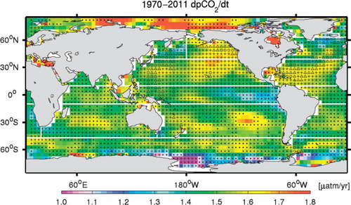
Fay and McKinley (2013) demonstrate in their study that due to internal climate variability, short-term surface pCO₂ trends are sensitive to the beginning and end dates of the observations and do not necessarily reflect the long-term trends. Consequently, we have focused on estimating the long-term regional pCO₂ trends over a period of four decades. Over this time scale, the estimated pCO₂ trends should be representative of the ocean's long-term response (i.e. ocean carbon sink) to the increasing atmospheric CO₂. Differing from previous observation-based studies, Fay and McKinley (2013) applied ocean biogeochemical general circulation models to verify the robustness of the estimated regional pCO₂ trends at various time scales. This study extends that work by testing the sensitivity of the computed regional trends to the observed data sampling, and investigating what role this plays in explaining the trend. For example, in the Atlantic sector of the Southern Ocean, consistent with Fay and McKinley (2013) we see that our observation-based estimate of the long-term pCO₂ trend is considerably lower than the atmospheric pCO₂ trend. Here, our model analysis indicates that this could be related to the very sparse data in large portion of this region (see for example, Fig. 10).

Fig. 10 Map illustrating the spatial and temporal observational coverage on top of model-mean pCO₂ trend for the 1970–2011 period. The grid cells with (·), (+), (Δ), and (°) indicate that there are 1–10, 11–50, 51–100, and more than 100 monthly pCO₂ observations, respectively.

Our analysis assesses the regional pCO₂ trend estimates and their driving mechanisms over the historical period, which gives us confidence to extend our analysis into the future, particularly over the last 40 yr of the 21st century as projected by the ESMs under the RCP8.5. Through analysing the future pCO₂ trend relative to the atmospheric pCO₂ growth rate, we highlight the growing potential of using long-term observations of surface ocean pCO₂ to detect and elucidate the climate system response to the anthropogenic forcings. Here, we identify regions where the pCO₂ trends are expected to deviate the most from the respective atmospheric trends, hence allowing us to detect signal change or potential feedback mechanism associated with future climate change.

4.2. Regional subsampling

We make use of the latest ensemble of ESM simulations both to evaluate model performance and to explore the regional trend uncertainties related to sampling coverage. These models are part of phase five of the Coupled Model Intercomparison Project (CMIP5) and also contribute to the recent Fifth Assessment Report of the Intergovernmental Panel on Climate Change (IPCC-AR5). Despite differences in model components, all models analysed here were able to reasonably reproduce the observed long-term mean spatial pCO₂ variability. Consistent with the observations, model-derived long-term pCO₂ trends are also positive and slightly weaker than the atmospheric pCO₂ growth rate over the last four decades.

In the contemporary period, the model simulated regional pCO₂ trends agree with the observed trends in only 5 of the 14 regions analysed here. However, when the model output is sampled at the same spatial and temporal resolution as the observations, the subsampled trends are indistinguishable from the observations in 12 regions (see Fig. 3). This result gives us more confidence in the model simulations. More importantly, the subsampling exercise shows that, due to limitation in data coverage, the observationally derived trends may be slightly biased when extrapolated over larger ocean basins. To illustrate this, we have plotted a map of spatial observational coverage together with the gridded pCO₂ trends from the model mean for the 1970–2011 period, as shown in Fig. 10. Figure 10 also includes the boundaries separating the different ocean regions defined in this study. It displays several regions where the computed basin-scale trends are likely to come with large uncertainties due to the spatial coverage. For example, in the subtropical South Pacific and Indian, there are more observations in the western part than in the central and eastern parts of the gyres. The model mean shows that surface pCO₂ tends to increase faster in the eastern part of these gyres, and for this reason, the observation-based estimates in these regions may be biased towards the low side. The sparse spatial coverage in the Southern Ocean also makes it difficult to produce an accurate pCO₂ trend that is representative of this complex region. On the other hand, in the subtropical North Pacific, despite the fact that grid cells with more than 50 monthly observations are concentrated in the far west of the basin, the subsampled model trend does not deviate too far from the fully sampled trend (Fig. 3). This can be attributed by the spatial pCO₂ trend of the SPNP basin, where both western and eastern parts of the basin contain grid cells with high trends. In addition, the good temporal coverage at the HOT station may also reduce the eastern–western imbalance. An artefact of the methodology we use is that the ‘true’ pCO₂ trends may be underestimated in regions with increased temporal coverage over the latter part of the sampling period. Such methodological artefacts are difficult to avoid without invoking assumptions about the mean and annual cycle of the ocean pCO₂ distribution.

Figure 3 also shows that in regions where there is sufficient data coverage (e.g. in the subtropical North Atlantic and western subpolar North Pacific), the subsampled model trends do not deviate as much from the fully sampled trends. Therefore, based on the present model simulations, the observation-based regional and short-term scale pCO₂ trends should not be extrapolated to infer how the ocean carbon sink has evolved over larger ocean basins or even on the global scale. Our study underlines that in order to produce robust estimates of the ocean carbon sinks from long-term pCO₂ trends, good coverage of surface pCO₂ measurements in both space and time in all parts of the world ocean is needed.

4.3. Evolution and drivers of pCO₂ trends

We use the models to quantify and decompose the simulated pCO₂ trends into four drivers (SST, SSS, DIC, and ALK). In addition, the evolution of the regional pCO₂ trends and their implications for the ocean carbon sinks are assessed. Our model analysis confirms that for the present-day period, the surface pCO₂ trends closely follow the atmospheric pCO₂ over most of the global ocean, even in the upwelling regions where older water masses that have not been exposed to anthropogenic CO₂ outcrop to the ocean surface (e.g. equatorial Pacific Ocean and parts of the Southern Ocean). Stronger pCO₂ growth rates than the atmospheric pCO₂ trend are typically simulated in the subtropical North Atlantic and in the eastern subtropical Pacific Ocean (see also Fig. 10). The largest uncertainty is in the Arctic, where three (two) of the models simulate pCO₂ trends faster (slower) than the atmospheric pCO₂ trend.

When the pCO₂ trend is decomposed, we show that the increase in surface DIC predominantly explains most of the simulated pCO₂ trends in all regions, except for the Arctic. For the future period, surface DIC increase would increase the pCO₂ by at least 97% in the Atlantic Ocean between 45°S and 40°N. Increase in pCO₂ trend due to ongoing sea surface warming can also be detected throughout all regions. The largest warming effect is simulated in the subpolar North Pacific where, by the end of the 21st century, at least 17% of the simulated pCO₂ trend can be attributed to the increase in SST. Since the ocean pCO₂ tracks the atmospheric pCO₂ closely, regions of higher warming rate have higher SST, hence lower DIC, contributions to the overall pCO₂ trend (e.g. WSPNP and ESPNP in Table 2).

As expected, the change in surface SSS only contributes marginally to the overall trends. The models also project an increase in evaporation in most parts of the Atlantic and an increase in precipitation over large parts of the Pacific and the Southern Ocean. The simulated change in surface freshwater flux is reflected in the change in surface ALK, and hence pCO₂ trend due to the dilution effect (i.e. higher ALK leads to lower pCO₂). We note that changes in the pCO₂ trends due to the dilution effect on ALK are to some extent balanced by an opposing dilution effect acting on the surface DIC in all ocean regions.

The basin-scale pCO₂ trends follow the atmospheric trends closely over the contemporary period in all regions. However, they are projected to deviate from one region to the other by the end of the 21st century. The Labrador Sea and the northeast Atlantic emerge as the regions with the fastest pCO₂ growth rate, faster than the atmospheric CO₂ trend by approximately 1 µatm yr⁻¹. This could be caused by the faster warming projected in this region and weakening of the Atlantic Meridional Overturning Circulation (AMOC, Cheng et al., 2013). On the contrary, regions such as the eastern equatorial Pacific, northwest subpolar North Pacific, and the high-latitude Southern Ocean are expected to have pCO₂ growth rates that are weaker than the atmospheric pCO₂ trend. The equatorial Pacific is an upwelling region, where relatively old water that has not been exposed to the elevated atmospheric pCO₂, is brought up to the ocean surface. In this region, the surface pCO₂ evolution would be less dependent on the atmospheric pCO₂ and more likely to be impacted by the ALK:DIC ratio of the source water. In regions where the water masses have spent more time at the surface and are thus more equilibrated with the atmospheric pCO₂ (e.g. the mid-latitudes), surface pCO₂ is more expected to track the atmospheric pCO₂ increase.

If we assume no significant changes in surface wind speed, the regional long-term surface pCO₂ trends and atmospheric pCO₂ measurements can be used to infer changes in the ocean CO₂ uptake rates. The lower oceanic than atmospheric pCO₂ trends over the last four decades imply that the ocean carbon uptake rate has continued to increase. At the end of the 21st century under the RCP8.5 scenario, the carbon uptake rate stabilizes and potentially weakens in some regions, particularly the subpolar North Atlantic. In low pCO₂ trend regions (e.g. the eastern equatorial Pacific and the high-latitude Southern Ocean), the uptake rate is expected to further increase.

Based on the model analysis, the observed multi-decadal trends in surface pCO₂ should be a good indicator of basin-scale changes in ocean carbon sinks, given sufficient spatial and temporal observational coverage. For example, four of five models simulate considerable shifts in 40-yr pCO₂ trends centred around year 2050, when the projected anthropogenic CO₂ emissions approach a constant value in the RCP8.5 scenario. This is also the period when the global ocean sink starts to slow down before it stabilizes towards the end of the 21st century. The challenge is then to accurately observe long-term pCO₂ trends representative of the global or key large-scale ocean basins.

4.4. Limitations and recommendations

A better understanding of the fate of anthropogenic carbon after it enters the ocean could help to elucidate the regional variations in the pCO₂ trend presented in this study. For example, Tjiputra et al. (2010) used a model to evaluate the lateral transport of anthropogenic carbon between different ocean basins. They show that in the high-latitude Southern Ocean, most of the anthropogenic carbon taken up from the atmosphere would be exported northward. Thus, the accumulation of anthropogenic carbon here is relatively low, and it is not surprising that the high-latitude Southern Ocean will be one of the few regions with a pCO₂ trend that remains below the atmospheric trend by the end of the 21st century. By contrast, in addition to anthropogenic carbon uptake through air–sea gas exchange, Tjiputra et al. (2010) also simulate a large accumulation of anthropogenic carbon through lateral transport into the North Atlantic basin associated with the meridional overturning circulation. Here we show that the subpolar North Atlantic is expected to have the largest pCO₂ trend. We note that, at present, there is no study that quantifies the impact of anthropogenic carbon transport due to circulation on surface pCO₂, and therefore more research in this area is required.

Another limitation of our study is that we analyse only the annual mean pCO₂ growth rate. Lenton et al. (2012) showed that investigating both the ocean pCO₂ growth rates and its drivers at the seasonal rather than annual scale can strongly bias our understanding of changes at the regional scale. Given that many of the largest changes in the carbon cycle occur at the seasonal scale (e.g. Rodgers et al., 2008; Gorgues et al., 2010), more work on investigating the observed and simulated seasonal changes is necessary.

We also acknowledge the limitations of the models, e.g. the simulated pCO₂ trend in the Arctic (ARC) comes with large inter-model spread. This uncertainty is likely attributed to complex physical-biogeochemical interactions, such as different heating rates, sea-ice formation and melting, changes in precipitation, riverine fluxes, among others. Quantification of these different physical contributions from the models is beyond the scope of this study. Furthermore, most models neither simulate ALK well nor consider ALK in the sea-ice and river runoff (Anderson et al., 2004; Anderson and Jones, 2012). Nevertheless, all models suggest that the change in freshwater flux in the Arctic through the dilution effect will be an important factor for the future surface pCO₂ evolution.

The good agreement between the observed and subsampled model trends is encouraging. Assimilation of the growing surface pCO₂ database into ocean biogeochemical general circulation models should be explored in order to obtain the best estimate of ocean carbon sinks from both models and data. Data assimilation will also be useful to identify model deficiencies as well as to evaluate the quality of the current observational networks.

Largely due to the extensive sampling programs in the North Atlantic and eastern mid-latitude North Pacific regions, the long-term feedback monitoring strategy of surface pCO₂ carried out in these regions over the last decades has been successful (e.g. Schuster and Watson, 2007; Olsen et al., 2008; Watson et al., 2009; Metzl et al., 2010; Nakaoka et al., 2013). We recommend that these are continued. Our analysis shows that these are some of the few regions expected to experience long-term surface pCO₂ growth rates that are faster than the atmospheric growth rates. While the subtropical North Pacific and subpolar North Atlantic have good temporal coverage, the spatial coverage needs to be improved. This also highlights the ongoing need to improve spatial and temporal coverage in regions such as the Southern and Indian Oceans. Our work also highlights the importance and need for a sustained long-term observing strategy to continue monitoring the ocean anthropogenic CO₂ sink and to better understand the potential carbon cycle feedbacks to climate that could arise from it. As demonstrated in this study, sustainable measurement programs have been proven to be valuable for the assessment of the latest collection of ESMs, which are one of the most widely used tools for projecting future climate change.

5. Conclusions

We have investigated the change in the ocean pCO₂ trends relative to the atmospheric pCO₂ trends over the historical and future periods, based on latest ESM simulations (CMIP5) and available upper ocean observations (1970–2011). Over the historical period, we find that the observed ocean trends are lower than the atmospheric growth rate of 1.61 µatm yr⁻¹ in all ocean regions, and range between 0.69 and 1.36 µatm yr⁻¹. Conversely, the simulated regional ocean pCO₂ trends track the atmospheric trend more closely (within 0.2 µatm yr⁻¹). However, when the models are subsampled with the observational coverage, we find good agreement between the simulated and the observed pCO₂ trends. This suggests: i) that despite the intense research programs, the spatial and temporal sampling frequency is not adequate to capture pCO₂ trends in most regions, and ii) that we have confidence in the trends simulated by the CMIP5 models over the historical period. Nevertheless, in some regions, in particular in the northern hemisphere, the observations allow us to establish the magnitude of the trends with some confidence. Due to these limitations, it remains challenging to confidently estimate the long-term ocean sink of anthropogenic CO₂ from the current observational network. Excluding the Arctic, the models show that change in DIC is the key driver of all regional pCO₂ trends (between 0.8 and 1.5 µatm yr⁻¹). Changes in ALK and SST contribute between −0.2 and 0.45 µatm yr⁻¹ and 0.1–0.4 µatm yr⁻¹ _, respectively, to the ocean pCO₂ trends.

Good model-data agreement in the simulated pCO₂ trends over the historical period gives us confidence in using CMIP5 model as tools to investigate how the ocean’s uptake of atmospheric CO₂ may evolve into the future. Towards the end of the 21st century, under the RCP8.5 scenario, more than 40% of the surface ocean area has a higher ocean than atmospheric pCO₂ trend, compared with approximately 10% over the contemporary period. The regions with the largest ocean pCO₂ trends are the subpolar North Atlantic and the subtropical gyres. It is in these regions where a reduction in the ocean CO₂ uptake capacity is expected to be strongest. In regions where the ocean circulation brings waters with low anthropogenic CO₂ concentrations to the ocean surface (the high-latitude Southern Ocean and the equatorial Pacific), the ocean pCO₂ trends are lower than the atmospheric trends. Here, ocean CO₂ uptake is expected to continue to increase, in agreement with previous studies (e.g. Caldeira and Duffy, 2000; Crueger et al., 2008; Roy et al., 2011). The positive trends in future ocean pCO₂ are predominantly driven by the increase in carbon concentration. Warming continues to increase pCO₂ trends in most regions, particularly in the subpolar North Pacific. Changes in the hydrological cycle make an increasingly important contribution to surface ocean pCO₂ trends in the future.

6. Acknowledgements

We thank three anonymous reviewers for their critical feedback, which helped to improve the manuscript significantly. The research leading to these results was supported by the Centre for Climate Dynamics at the Bjerknes Centre and the EU FP7 project CARBOCHANGE ‘Changes in carbon uptake and emissions by oceans in a changing climate’, which received funding from the European Commission's Seventh Framework Programme under grant agreement no. 264879. SOCAT, GLODAP, CARINA, and PACIFICA are international efforts supported by the International Ocean Carbon Coordination Project (IOCCP). The many researchers and funding agencies responsible for the collection of data and quality control are thanked for their contributions to the above data products. We acknowledge the World Climate Research Programme's Working Group on Coupled Modelling, which is responsible for CMIP5. For CMIP the U.S. Department of Energy's Program for Climate Model Diagnosis and Intercomparison provides coordinating support and led development of software infrastructure in partnership with the Global Organization for Earth System Science Portals. JFT acknowledges the Research Council of Norway funded project EarthClim (no. 207711/E10) and the NOTUR projects nn2980k and nn2345k as well as the NorStore projects ns2980k and ns2345k for supercomputer time and storage resources. AL acknowledges support from the Australian Climate Change Science Program. The collection of data from CLIVAR cruises was compiled and generously shared with us by Robert Key at Princeton University. The CESM1-BGC output was provided by Keith Lindsay.

Notes

To access the supplementary material to this article, please see Supplementary files under Article Tools online.

References

- Anderson L. G , Jones E. P . Measurements of total alkalinity, calcium, and sulfate in natural sea ice. J. Geophys. Res. Ocean. 2012; 90: 9194–9198.
- Anderson L. G , Jutterstrom S , Kaltin S , Jones E. P , Bjork G. R . Variability in river runoff distribution in the Eurasian Basin of the Arctic Ocean. J. Geophys. Res. 2004; 109: C01016.
- Anderson L. G , Olsson K , Chierici M . A carbon budget for the Arctic. Global Biogeochem. Cycles. 1998; 12: 455–465.
- Bakker D. C. E , Pfeil P , Smith K , Hankin S , Olsen A , co-authors . An update to the Surface Ocean CO2 Atlas (SOCAT version 2). Earth Syst. Sci. Data. 2014; 6: 69–90.
- Bates N. R . Multi-decadal uptake of carbon dioxide into subtropical mode water of the North Atlantic Ocean. Biogeosciences. 2012; 9: 2649–2659.
- Bates N. R , Best M. H. P , Neely K , Garley R , Dickson A. G , co-authors . Detecting anthropogenic carbon dioxide uptake and ocean acidification in the North Atlantic Ocean. Biogeosciences. 2012; 9: 2509–2522.
- Bopp L , Resplandy L , Orr J , Doney S. C , Dunne J. P , co-authors . Multiple stressors of ocean ecosystems in the 21st century: projections with CMIP5 models. Biogeosciences. 2013; 10: 6225–6245.
- Caldeira K , Duffy P. B . The role of the Southern Ocean in the uptake and storage of anthropogenic carbon dioxide. Science. 2000; 287: 620–622. [PubMed Abstract].
- Cheng W , Chiang J. C. H , Zhang D. X . Atlantic Meridional Overturning Circulation (AMOC) in CMIP5 models: RCP and historical simulations. J. Clim. 2013; 26: 7187–7197.
- Chierici M , Fransson A , Nojiri Y . Biogeochemical processes as drivers of surface fCO2 in contrasting provinces in the subarctic North Pacific Ocean. Global Biogeochem. Cycles. 2006; 20: GB1009.
- Crueger T , Roeckner E , Raddatz T , Schnur R , Wetzel P . Ocean dynamics determine the response of oceanic CO2 uptake to climate change. Clim. Dynam. 2008; 31: 151–168.
- Dickson A. G , Millero F. J . A comparison of the equilibrium constants for the dissociation of carbonic acid in seawater media. Deep-Sea Res. 1987; 34: 1733–1743.
- Dore J. E , Lukas R , Sadler D. W , Karl D. M . Climate-driven changes to the atmospheric CO2 sink in the subtropical North Pacific Ocean. Nature. 2003; 424: 754–757. [PubMed Abstract].
- Dufour C. O , Le Sommer J , Gehlen M , Orr J. C , Molines J.-M , co-authors . Eddy compensation and controls of the enhanced sea-to-air CO2 flux during positive phases of the Southern Annular Mode. Global Biogeochem. Cycles. 2013; 27: 950–961.
- Fay A. R , McKinley G. A . Global trends in surface ocean pCO2 from in situ data. Global Biogeochem. Cycles. 2013; 27: 1–7.
- Feely R. A , Takahashi T , Wanninkhof R , McPhaden M. J , Cosca C. E , co-authors . Decadal variability of the air-sea CO2 fluxes in the equatorial Pacific Ocean. J. Geophys. Res. 2006; 111: C08S90.
- GLOBALVIEW-CO2 . Cooperative Atmospheric Data Integration Project – Carbon Dioxide. 2012; Boulder, CO: NOAA ESRL. Online at: http://www.esrl.noaa.gov/gmd/ccgg/globalview/ .
- Gorgues T , Aumont O , Rodgers K. B . A mechanistic account of increasing seasonal variations in the rate of ocean uptake of anthropogenic carbon. Biogeosciences. 2010; 7: 2581–2589.
- Gruber N . Carbon cycle: fickle trends in the ocean. Nature. 2009; 458: 155–156. [PubMed Abstract].
- Jones C , Robertson E , Arora V , Friedlingstein P , Shevliakova E , co-authors . Twenty-first-century compatible CO2 emissions and airborne fraction simulated by CMIP5 Earth system models under four representative concentration pathways. J. Clim. 2013; 26: 4398–4413.
- Keller K , Joos F , Raible C , Cocco V , Frölicher T , co-authors . Variability of the ocean carbon cycle in response to the North Atlantic Oscillation. Tellus B. 2012; 64: 18738.
- Key R. M , Kozyr A , Sabine C. L , Lee K , Wanninkhof R , co-authors . A global ocean carbon climatology: results from Global Data Analysis Project (GLODAP). Global Biogeochem. Cycles. 2004; 18: 4031.
- Key R. M , Tanhua T , Olsen A , Hoppema M , Jutterström S , co-authors . The CARINA data synthesis project: introduction and overview. Earth Syst. Sci. Data. 2010; 2: 105–121.
- Lee K , Tong L. T , Millero F. J , Sabine C. L , Dickson A. G , co-authors . Global relationships of total alkalinity with salinity and temperature in surface waters of the world's oceans. Geophys. Res. Lett. 2006; 33: L19605.
- Lenton A , Matear R. J . The role of the Southern Annular Mode (SAM) in Southern Ocean CO2 uptake. Global Biogeochem. Cycles. 2007; 21: GB2016.
- Lenton A , Metzl N , Takahashi T , Kuchinke M , Matear R. J , co-authors . The observed evolution of oceanic pCO2 and its drivers over the last two decades. Global Biogeochem. Cycles. 2012; 26: GB2021.
- Lenton A , Tilbrook B , Law R. M , Bakker D , Doney S. C , co-authors . Sea–air CO2 fluxes in the Southern Ocean for the period 1990–2009. Biogeosciences. 2013; 10: 4037–4054.
- Le Quéré C , Andres R. J , Boden T , Conway T , Houghton R. A , co-authors . The global carbon budget 1959–2011. Earth Syst. Sci. Data. 2013; 5: 185–185.
- Le Quéré C , Takahashi T , Buitenhuis E. T , Rödenbeck C , Sutherland C . Impact of climate change and variability on the global oceanic sink of CO2 . Global Biogeochem. Cycles. 2010; 24: GB4007.
- Lovenduski N. S , Gruber N , Doney S. C . Toward a mechanistic understanding of the decadal trends in the Southern Ocean carbon sink. Global Biogeochem. Cycles. 2008; 22: GB3016.
- Lovenduski N. S, Gruber N , Doney S. C , Lima I. D . Enhanced CO2 outgassing in the Southern Ocean from a positive phase of the Southern Annular Mode. Global Biogeochem. Cycles. 2007; 21: GB2026.
- Marinov I , Gnanadesikan A , Toggweiler J. R , Sarmiento J. L . The Southern Ocean biogeochemical divide. Nature. 2006; 441: 964–967. [PubMed Abstract].
- McKinley G. A , Fay A. R , Takahashi T , Metzl N . Convergence of atmospheric and North Atlantic carbon dioxide trends on multidecadal timescales. Nat. Geosci. 2011; 4: 606–610.
- Mehrbach C , Culberson C. H , Hawley J. E , Pytkowicz R. M . Measurement of the apparent dissociation constants of carbonic acid in seawater at atmospheric pressure. Limnol. Oceanogr. 1973; 18: 897–907.
- Metzl N , Corbière A , Reverdin G , Lenton A , Takahashi T , co-authors . Recent acceleration of sea surface fCO2 growth rate in the North Atlantic subpolar gyre (1993–2008) revealed by winter observations. Global Biogeochem. Cycles. 2010; 24: GB4004.
- Moss R. H , Edmonds J. A , Hibbard K. A , Manning M. R , Rose S. K , co-authors . The next generation of scenarios for climate change research and assessment. Nature. 2010; 463: 747–756. [PubMed Abstract].
- Nakaoka S , Telszewski M , Nojiri Y , Yasunaka S , Miyazaki C , co-authors . Estimating temporal and spatial variation of ocean surface pCO2 in the North Pacific using a self-organizing map neural network technique. Biogeosciences. 2013; 10: 6093–6106.
- Olsen A , Brown K. R , Chierici M , Johannessen T , Neill C . Sea-surface CO2 fugacity in the subpolar North Atlantic. Biogeosciences. 2008; 5: 535–547.
- Omar A. M , Olsen A . Reconstructing the time history of the air-sea CO2 disequilibrium and its rate of change in the eastern subpolar North Atlantic. Geophys. Res. Lett. 2006; 33: L04602.
- Peters G. P , Andrew R. M , Boden T , Canadell J. G , Ciais P , co-authors . The challenge to keep global warming below 2 °C. Nat. Clim. Change. 2012; 3: 4–6.
- Pfeil B , Olsen A , Bakker D. C. E, Hankin S , Koyuk H , co-authors . A uniform, quality controlled Surface Ocean CO2 Atlas (SOCAT). Earth Syst. Sci. Data. 2013; 5: 125–143.
- Pierrot D , Neill C , Sullivan K , Castle K , Wanninkhof R , co-authors . Recommendations for autonomous underway pCO2 measuring systems and data-reduction routines. Deep-Sea Res. Pt. II. 2009; 56: 512–522.
- Rodgers K. B , Sarmiento J. L , Aumont O , Crevoisier C , de Boyer Montegut C , co-authors . A wintertime uptake window for anthropogenic CO2 in the North Pacific. Global Biogeochem. Cycles. 2008; 22: GB2020.
- Roy T , Bopp L , Gehlen M , Schneider B , Cadule P , co-authors . Regional impacts of climate change and atmospheric CO2 on future ocean carbon uptake: a multimodel linear feedback analysis. J. Clim. 2011; 24: 2300–2318.
- Sabine C. L , Hankin S , Koyuk H , Bakker D. C. E , Pfeil B , co-authors . Surface Ocean CO2 Atlas (SOCAT) gridded data products. Earth Syst. Sci. Data. 2013; 5: 145–153.
- Schuster U , McKinley G. A , Bates N , Chevallier F , Doney S. C , co-authors . An assessment of the Atlantic and Arctic sea–air CO2 fluxes, 1990–2009. Biogeosciences. 2013; 10: 607–627.
- Schuster U , Watson A. J . A variable and decreasing sink for atmospheric CO2 in the North Atlantic. J. Geophys. Res. 2007; 122: 11006.
- Stott P. A , Sutton R. T , Smith D. M . Detection and attribution of Atlantic salinity changes. Geophys. Res. Lett. 2008; 33: 21702.
- Suzuki T , Ishii M , Aoyama M , Christian J. R , Enyo K , co-authors . PACIFICA Data Synthesis Project. ORNL/CDIAC-159, NDP-092. 2013. [PubMed CentralFull Text] Carbon Dioxide Information Analysis Center, Oak Ridge National Laboratory, U.S. Department of Energy, Oak Ridge, Tennessee.
- Takahashi T , Sutherland S. C , Feely R. A , Wanninkhof R . Decadal change of the surface water pCO2 in the North Pacific: a synthesis of 35 years of observations. J. Geophys. Res. 2006; 111: 07S05.
- Takahashi T , Sutherland S. C , Wanninkhof R , Sweeney C , Feely R. A , co-authors . Climatological mean and decadal change in surface ocean pCO 2 , and net sea–air CO2 flux over the global oceans. Deep Sea Res. Part II. 2009; 56: 664–577.
- Takahashi T , Sweeney C , Sutherland S. C . Underway pCO2 Measurements in Surface Waters and the Atmosphere During the R/V Laurence M. Gould Expeditions. 2011. Online at: http://cdiac.ornl.gov/ftp/oceans/VOS\_Gould\_Lines/. Carbon Dioxide Information Analysis Center, Oak Ridge National Laboratory, US Department of Energy, Oak Ridge, Tennessee [PubMed CentralFull Text].
- Taylor K. E , Stouffer R. J , Meehl G. A . An overview of CMIP5 and the experiment design. Bull. Am. Meteorol. Soc. 2012; 93: 485–498.
- Thomas H , Friederike Prowe A. E , Lima I. D , Doney S. C , Wanninkhof R , co-authors . Changes in the North Atlantic Oscillation influence CO2 uptake in the North Atlantic over the past 2 decades. Global Biogeochem. Cycles. 2008; 22: 4027.
- Tjiputra J. F , Assmann K , Heinze C . Anthropogenic carbon dynamics in the changing ocean. Ocean Sci. 2010; 6: 605–614.
- Tjiputra J. F , Olsen A , Assmann K , Pfeil B , Heinze C . A model study of the seasonal and long-term North Atlantic surface pCO2 variability. Biogeosciences. 2012; 9: 907–923.
- Watson A. J , Schuster U , Bakker D. C. E , Bates N. R , Corbiere A , co-authors . Tracking the variable North Atlantic sink for atmospheric CO2 . Science. 2009; 326: 1391–1393. [PubMed Abstract].
- Wong C. S , Johannessen S . Sea surface and atmospheric pCO2 data in the Pacific Ocean during the Station P cruises from 1973–2003. 2010. Online at: http://cdiac.ornl.gov/ftp/oceans/station_p_ca/. Carbon Dioxide Information Analysis Center, Oak Ridge National Laboratory, US Department of Energy, Oak Ridge, Tennessee [PubMed CentralFull Text].