Past and future carbon fluxes from land use change, shifting cultivation and wood harvest

Abstract

Carbon emissions from anthropogenic land use (LU) and land use change (LUC) are quantified with a Dynamic Global Vegetation Model for the past and the 21st century following Representative Concentration Pathways (RCPs). Wood harvesting and parallel abandonment and expansion of agricultural land in areas of shifting cultivation are explicitly simulated (gross LUC) based on the Land Use Harmonization (LUH) dataset and a proposed alternative method that relies on minimum input data and generically accounts for gross LUC. Cumulative global LUC emissions are 72 GtC by 1850 and 243 GtC by 2004 and 27–151 GtC for the next 95 yr following the different RCP scenarios. The alternative method reproduces results based on LUH data with full transition information within <0.1 GtC/yr over the last decades and bears potential for applications in combination with other LU scenarios. In the last decade, shifting cultivation and wood harvest within remaining forests including slash each contributed 19% to the mean annual emissions of 1.2 GtC/yr. These factors, in combination with amplification effects under elevated CO₂, contribute substantially to future emissions from LUC in all RCPs.

• land use change
• carbon cycle
• carbon budget
• wood harvest
• shifting cultivation
• terrestrial carbon sink

1. Introduction

Land use (LU) and land use change (LUC) are generally associated with a reduction in vegetation (Baccini et al., 2012; Harris et al., 2012) and, to a varying degree, soil carbon (C) storage (Guo and Gifford, 2002), resulting in carbon emissions to the atmosphere (Watson et al., 2000; McGuire et al., 2001; Houghton et al., 2012). LUC and LU not only affect the cycling of C, but also impact nutrients, such as nitrogen (N) and phosphorous (P), the emissions of greenhouse gases from soils (e.g., N₂O, CH₄), and emissions of chemical reactive compounds, in particular by LUC-related fires. The modification of the land surface by LUC also affects biogeophysical properties, such as albedo, water, and energy fluxes (Claussen et al., 2001; Feddema et al., 2005; Bala et al., 2007). LUC was shown to affect the seasonal variation in temperature, and precipitation patterns, snow cover in high latitude regions, and atmospheric dynamics, and entails consequences on biodiversity and socio-economic aspects (IUCN, 2000; UNEP, 2002). In the following, we refer to ‘LU’ as the direct impact of human activities on terrestrial ecosystems without the aspect of its change over time. Indirect impacts such as the effects of climate change or air pollution are not included. The temporal change in LU is referred to as ‘LUC’.

Hurtt et al. (2006) suggest that 42–68% of the land surface has been affected by conversion to croplands and pastures and by wood harvesting since 1700 (years always referred to as AD). Parallel expansion and abandonment of agricultural land (shifting cultivation), afforestation, wood harvesting and successive recovery leaves behind a vast area of secondary land where biogeochemical cycling and biogeophysical properties are altered and only re-generate to ‘natural’ conditions on time scales of decades to centuries (Houghton et al., 1983). Such legacy effects co-determine the terrestrial C balance and the human impact on the C cycle, but this complexity is often not or only partly taken into account (Brovkin et al., 2013) due to a lack of information determining the myriad transitions between different LU categories and the methodological challenges of its implementation in land carbon cycle models.

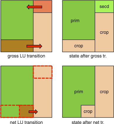
Hurtt et al. (2006) combined satellite data, and national forestry and agriculture statistics with assumptions for the land turnover rate and the spatial distribution of shifting cultivation in a dataset [Land Use Harmonization (LUH)], defining the evolution of the area under LU and all transitions between LU categories. Thus, the LUH data provide information which represents shifting cultivation as bi-directional (gross) LU transitions. For example, the conversions from forest to cropland and vice versa are considered individually, whereas traditional ‘static’ LU maps provide only net changes in an area (see Fig. 1).

Fig. 1 Schematic illustration of simulating gross versus net land use change (LUC). Under a scheme for gross LUC (upper row), cropland is claimed from primary land (‘prim’) and abandoned to secondary land (‘secd’) in parallel within one grid cell. In the model, croplands and pasture areas undergo gross LUC in areas of shifting cultivation. Under a scheme for net LUC (lower row), only the difference of claimed minus abandoned undergoes a transition to use as cropland and no separate secondary land is formed. In the latter scheme, a smaller grid cell area fraction is affected by LUC.

The concept of gross LU transitions can also accommodate wood harvesting as a transition from and to forested (non-agricultural) land, not captured when only accounting for net LUC. The cumulative removal of harvested biomass was estimated by Houghton (1999) to 106 GtC (1850–1990), plus 149 GtC of slash that was produced additionally. Hurtt et al. (2006) (LUH) provide similar estimates for this period. They reconstruct 100 GtC of cumulative harvested biomass, including slash, plus an additional biomass loss from land conversion of 105 GtC based on the HYDE, or 153 GtC based on SAGE/HYDE LU maps. This relatively large difference is linked to the dynamics of land turnover and the spatial distribution of areas under shifting cultivation and illustrates its potency in affecting LUC emission estimates.

Wood harvest results in a C flux out of the terrestrial biosphere in the order of 1 GtC/yr at present (Hurtt et al., 2006). However, land affected by wood harvest and abandoned agricultural land acts as a C sink during vegetation regrowth and the net effect is much smaller. Still, the general reduction of C stocks in forests affected by wood harvest implies an additional C source. The combined additional sources from wood harvest and shifting cultivation have been estimated by Houghton (2010) to 28%, and by Shevliakova et al. (2009), who applied the LUH dataset for the past, to 40–49% (1700–2000). Olofsson and Hickler (2008) estimated a contribution by shifting cultivation effects alone of 26% for the period since the appearance of early agriculture.

Other published LUC model simulations based on LUH and covering the Representative Concentration Pathways (RCPs) (van Vuuren et al., 2011a) for the 21st century either report LUC-induced changes in above-ground biomass only (Hurtt et al., 2011), or present global total net ecosystem exchange where LUC emissions are not separated from fluxes resulting from other drivers (Lawrence et al., 2012). Brovkin et al. (2013) presented results from six, state-of-the-art, CMIP5 Earth System Models, of which only one model [MPI-ESM-LR, Reick et al. (2013)] accounted for both wood harvest, and gross transitions. This model suggests the highest future LUC emissions, but effects of shifting cultivation and wood harvest have not been separated from other aspects (e.g., vegetation C density).

Historical LU reconstructions are uncertain (Gaillard et al., 2010), and assessments of the impact on the pre-industrial carbon cycle ideally rely on considering different contrasting reconstructions [HYDE (Klein Goldewijk et al., 2011), SAGE (Ramankutty and Foley, 1999) and Kaplan et al. (2011)] or multiple scenarios (Stocker et al., 2011). However, the assessment of the impact of shifting cultivation is still restricted by the limited data on bi-directional transitions (so far, only the LUH dataset provides this information), while static LU maps are available for a range of different reconstructions (Pongratz et al., 2008; Kaplan et al., 2011; Klein Goldewijk et al., 2011) and for periods not covered by LUH.

Here, we simulate carbon emissions from gross LU transitions in the nitrogen-enabled Land surface Processes and eXchanges (LPX-Bern 1.0) Dynamic Global Vegetation Model (DGVM), forced by LU input data from Hurtt et al. (2006, 2011), based on the HYDE data (Klein Goldewijk et al., 2011). In our analyses, we focus particularly on the contribution of land turnover and wood harvest to LUC emissions and extend the scope of earlier studies by addressing these effects in all four RCPs based on the LUH dataset.

Thus, the goal of this study is also to develop and apply an alternative method to include shifting cultivation and wood harvest in other, static LU reconstructions. This method avoids problems with artefact fluxes related to model spin-up and varying transition priorities when using the LUH dataset.

2. Methods

2.1. LU transition model

The LUH dataset incorporates the HYDE 3.1 static LU maps of cropland, pastures and urban areas (Klein Goldewijk et al., 2011). In addition, LUH distinguishes the remaining natural land in primary and secondary, and resolves net LUC into bi-directional area transitions. Secondary land is defined as natural land, previously disturbed by and recovering from anthropogenic activity (Hurtt et al., 2006). LU areas are given as the fraction of each grid cell occupied by LU category k, at year t, and will be referred to as ‘LU states’. Area transitions denote the fractional areas converted from category l to category k and will be referred to as ‘LU transitions’. The LUH dataset is provided on a 0.5°×0.5° spatial resolution. For the present application, the data is converted to 1°×1° resolution conserving the absolute area in each LU category and transition within each grid cell on the coarse resolution.

The transitions are composed of three components of a transition matrix ΔA [(eq. (1)] and must satisfy the constraint given in eq. (2) below:1 2

ΔA _net is a matrix describing minimal area transitions to satisfy the net change in LU areas between two time steps [eq. (2)]. These ‘net LU transitions’ are comparable to the representation of LUC in earlier studies (Strassmann et al., 2008; Stocker et al., 2011). In contrast, C pools on secondary land are explicitly tracked here. ΔA _lato represents the additional transitions (land turnover) under shifting cultivation-type agriculture, where crop and pasture land is abandoned and re-claimed in parallel. ΔA _lato does not lead to a net change in area covered by the respective LU category. ΔA _harvest is a diagonal matrix for area transitions representing wood harvesting. It affects the LU categories ‘primary’ and 'secondary’ and describes by how much the tree cover and thus the number of trees and carbon stocks in living vegetation are reduced in each of these categories. In other words, ΔA _kk undergoes LUC but does not change the LU category. ΔA _harvest is determined interactively on the basis of LUH input data for the C mass harvested per grid cell and year and the simulated vegetation C density in LPX. Deforested wood biomass associated with the conversion ΔA _net +ΔA _lato is not counted towards satisfying wood harvest statistics.

Vegetation, litter, and soil pools are treated separately in each fractional land area (tile) and grid cell. C and N mass of soil and litter pools, and soil water on extending and contracting source area fractions are reallocated and mixed with pools on destination land area fractions () to conserve total mass. Vegetation C and N on contracting is diminished by reducing the number of individual trees and associated C and N mass of sapwood and heartwood pools is divided up between product pools of different turnover times, while C and N in leaves and roots are directed to the above- and below-ground litter pools of destination land area fractions (see Table 1 and Appendix).

Table 1. Split of C and N mass into slash (on-site litter pools) and product pools of different turnover times (0 yr, 2 yr, 20 yr) after deforestation (in% of deforested and harvested tree biomass)

		Product pools
	Slash	0 yr	2 yr	20 yr
Roots	100	0	0	0
Leaves	100	0	0	0
Sapwood	0	37.5	37.5	25
Heartwood	0	37.5	37.5	25

Management on agricultural land (crop and grass harvest) is implemented as a fraction f ^ox of above-ground biomass turnover that is directly oxidised, instead of being diverted to the litter pool. This approach broadly follows Shevliakova et al. (2009). Respective values for cropland and pasture harvesting are (). Additionally, the soil turnover rate is increased by 20% on croplands relative to non-cropland soils to account for accelerated oxidation of soil organic matter due to soil management, e.g., tillage [see Spahni et al. (2013)]. This implies a reduction of soil C on croplands in the order of 30% and no consistent change on pastures and is in general agreement with observational studies (Davidson and Ackerman, 1993; Guo and Gifford, 2002; Murty et al., 2002; Ogle et al., 2005).

The dynamics and interactions of C, N, and water pools are simulated by the LPX-Bern 1.0 DGVM (Spahni et al., 2013; Stocker et al., 2013) on a 1°×1° spatial resolution. LPX is based on the Lund-Potsdam-Jena (LPJ) DGVM (Sitch et al., 2003), includes a dynamical N cycle (Xu-Ri and Prentice, 2008), and builds on LUC representations as detailed by Strassmann et al. (2008) and Stocker et al. (2011). However, it differs from these earlier representations by accounting for shifting cultivation and harvest as described above, and also accounts for the distinction between C and N pools on primary versus secondary land (the process formulations and parameter values are identical for the two LU categories). N limitation is relaxed on agricultural land due to N fertiliser application.

2.2. Generated transitions

Alternative to the LUH data, we calculate ΔA using the maps and data on (1) the spatial distribution of shifting cultivation, (2) the land turnover rate, and (3) a priority list defining from which LU category area is claimed to satisfy expansion in another LU category (see Table 2). We apply rules (1)–(3) following Hurtt et al. (2006) as closely as possible. This method is termed ‘generated transitions (GNT)’ and will be referred to as GNT. The algorithms implemented in LPX are described as follows.

Table 2. Generated transitions priorities

→	Croplands	Pasture	Built-up
Primary	1	6	10
Secondary	2	5	9
Croplands	–	7	12
Pasture	3	–	11
Built-up	4	8	–

Numbers represent priority of transitions executed to satisfy net land use area changes (transition priorities associated with land turnover are in bold). Cropland and pasture area abandoned due to land turnover is always transferred to secondary (not shown here).

ΔA can be decomposed as detailed in eq. (1), where is constructed from A ^t−1 and A ^t and describes minimal area transitions to satisfy the net change in LU areas between two time steps. The algorithm applied to construct subsequently determines necessary transitions k→l in the order defined by Table 2. For example, if between two given years’ LU states, cropland expands while primary is reduced, then the respective transition is calculated first (‘1’ in Table 2) and ΔA _{net prim,crop} is set. If the cropland expansion is not fully met by this transition, then additional land is claimed from secondary, pasture or built-up land in this order, given the respective category is contracting between the two time steps.

In a second step, is generated based on the dataset for LU states and using information (1)–(3). The order in which transitions k→l are determined is given by the numbers in bold print in Table 2. Land is claimed from LU category k and allocated to l in order to compensate for land abandonment in l. The respective matrix element of ΔA _lato is defined as the minimum of required land for l and available land in k:3

λ is the land turnover rate, here set to 1/15 yr⁻¹ in areas of shifting cultivation and zero elsewhere. Land turnover rate and the spatial extent of shifting cultivation areas are adopted from the LUH data. If required land is not satisfied by available land in k (), then land is claimed from the category of second priority (see Table 2).

Land to be abandoned and allocated to secondary land (‘secd’) is determined after calculating eq. (3) to guarantee that abandonment does not exceed actual claimable land.4

This sequence of eqs. (3) and (4) is applied for l =(croplands, pastures) in this order (see also Table 2).

All natural land affected by ΔA _lato at any point during the simulation is considered secondary land. Its extent therefore depends on the starting year of the simulation and the duration of the model spin-up. is constructed analogously as described in Section 2.1. In Section 3, we compare results based on the GNT method with results using the LUH data.

2.3. Modelling protocol

The model is spun up for 1500 yr using A of 1500, i.e., a fixed distribution of primary, secondary, and agricultural land based on the LUH data, and ΔA=0. In spin-up year 1000, an analytical solution is applied to equilibrate soil C and organic N pools. During the last 300 yr of the spin-up, we apply a transition matrix ΔA*(1500), derived from ΔA (1500) but corrected so that no net changes in ΔA result. Thus, the distribution of the different land categories remains fixed. The secondary land fraction is zero during the spin-up and at the beginning of the transient simulation, as given by the LUH data. In the GNT method, we follow a similar procedure, except that secondary land is created during the last 300 yr of the spin-up as a result of continuous land turnover under shifting cultivation.

The LUC-related C flux to the atmosphere is evaluated from simulations with and without LUC (e _LU =−ΔC _LU+ΔC _noLU), where the carbon uptake by the terrestrial biosphere ΔC is calculated as the net ecosystem production minus the carbon release from product pools. In the standard setup (gross, including wood harvest) the full transition matrix, ΔA, is prescribed. Two additional simulations are used to attribute emissions to net area change, to land turnover, and to wood harvest. The effect of land turnover is calculated as the difference from a simulation where ΔA _net +ΔA _lato is used and one where LUC is simulated as in Stocker et al. (2011) (similar as using only ΔA _net). The effect of wood harvest is derived as the difference between the standard setup (full matrix ΔA) and the setup using ΔA _net +ΔA _lato.

Climate (temperature, precipitation, cloud cover, wet days) is prescribed from the CRU TS 3.20 data (Mitchell and Jones, 2005) for years 1901–2004, while for preceding years of the simulations (1500–1900), the first 31 yr of the CRU TS 3.20 dataset are recycled (constant climate). CO₂ is prescribed from observational data according to the CMIP5 protocol (MacFarling Meure et al., 2006; Taylor et al., 2012) with values held constant at 278 ppm before 1765. For the future period (2005–2099), CO₂ is prescribed from the RCP data (RCP database, 2009; van Vuuren et al., 2011a), while climate change is prescribed from the CMIP5 output of the IPSL-CM5A-LR model (Dufresne et al., 2013). This model features a moderate polar amplification of temperature change and yields intermediate results when prescribing its climate change pattern to simulate the terrestrial C balance changes and greenhouse gas emissions with LPX (Stocker et al., 2013). Prescribing changes in climate and CO₂ yields total emissions. Primary emissions are quantified from simulations with constant pre-industrial climate (recycled first 31 yr of the CRU TS 3.20 dataset throughout the entire simulation) and CO₂ (278 ppm, corresponding to the initial value in the applied CO₂ time series data set). Individual effects of climate (CO₂) are assessed with simulations where only CO₂ (climate) is held constant at pre-industrial levels. In all simulations, N deposition from Lamarque et al. (2011) and inorganic N fertiliser inputs from Zaehle et al. (2011) and Stocker et al. (2013) are prescribed.

3. Results

3.1. Past emissions

Total cumulative LUC emissions reach 72 GtC (GNT: 66 GtC, see section 3.3) by 1850 (including pre-1500 losses) and 243 GtC (GNT: 231) by 2004. Total LUC fluxes decrease from 1.55 GtC/yr and 1.57 GtC/yr in the 1980s and 1990s to 1.21 GtC/yr in the 2000s (Table 3, Fig. 2). These estimates are comparable with other studies (Pan et al., 2011; Stocker et al., 2011; Houghton et al., 2012).

Fig. 2 Historical annual LUC fluxes. Splined annual fluxes (thick colour lines) and year-by-year data for ‘gross, incl. wood harvest’ (thin grey line) are shown. The dashed lines (‘land turnover contribution’ and ‘wood harvest contribution’) are the differences between the respective curves (‘land turnover contribution’=‘gross, no wood harvest’ –‘net’; ‘wood harvest contribution’ =‘gross, incl. wood harvest’ –‘gross, no wood harvest’).

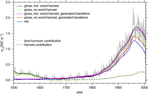
Table 3. Cumulative LUC emissions (E, [GtC]) and decadal average annual LUC fluxes (e, [GtC yr⁻¹]

	E [GtC]		e [GtC yr^−1]
	−1850	1850–2004	1980s	1990s	2000s
Total LUH	72	171	1.55	1.57	1.21
Total GNT	66	165	1.53	1.63	1.28
Primary LUH	70	154	1.48	1.27	0.99
CO2 effect		+21	+0.36	+0.41	+0.43
Climate effect		−4	−0.27	−0.11	−0.19
Climate & CO2		+17	+0.07	+0.30	+0.22
Wood harvest	+7	+23	+0.26	+0.27	+0.23
Land turnover	+20	+25	+0.21	+0.26	+0.23

Individual effects from CO₂, climate, wood harvest, and land turnover (shifting cultivation) are quantified only for the LUH dataset. Effects from climate are zero before 1850 by design (constant climate before 1901) and are not provided for CO₂ (constant atmospheric concentration prescribed before 1765).

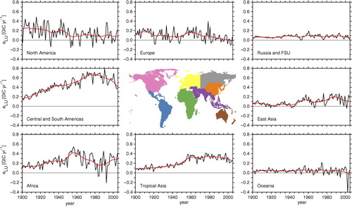
While LUC represents a source of C on the global scale, the picture is regionally more heterogeneous (see Fig. 3). For example, in Europe LUC represented a source of 15 TgC/yr during the 1980s and was a small sink of 3 TgC/yr over the period 2000–2004. LUC emissions have been increasing in Africa, in tropical and East Asia, as well as in Central and South America during the first part of the 20th century, but levelled off thereafter, showing a declining trend today in Latin America and the Asian regions.

Fig. 3 Annual LUC fluxes by region (black curves) and their splined time series (red curve). The regions are illustrated by the map in the middle and correspond to the delineation used in IPCC AR5 (Ciais et al., 2013), except that ‘Eurasia’ is separated into Europe (everything west of 60°E), and Russia and the Former Soviet Union (FSU) (everything east of 60°E).

The contribution of land turnover and wood harvest to the total LUC emissions is considerable (Table 3). It amounts to 37% for the pre-1850 period, to 28% for the period 1850–2004 and reaches 38% during the last decade. These contributions are broadly consistent with earlier estimates (Olofsson and Hickler, 2008; Shevliakova et al., 2009) and demonstrate that these processes should not be neglected.

Land turnover and wood harvesting leave a large area of forests affected by and recovering from previous anthropogenic disturbance. Consequently, C pools on non-agricultural land are generally smaller in regions where shifting cultivation occurs. This implies larger cumulative net emissions as well as larger gross fluxes (deforestation and regrowth fluxes) between the land and the atmosphere with deforestation. We quantify a ‘regrowth’-flux as the amplification of the C fluxes entering the land biosphere (NPP) due to LUC and a ‘deforestation’ flux (including the legacy of amplified respiration in response to past LUC) as the LUC-induced amplification of C fluxes leaving the land biosphere (heterotrophic respiration, fire, product decay). These fluxes are 7.4 GtC/yr (deforestation) and 6.0 GtC/yr (regrowth) in the standard simulation (mean over 1990–2004), but only 6.2 GtC/yr (deforestation) and 5.3 GtC/yr (regrowth) in the simulation where only net LUCs are simulated. Thus, shifting cultivation leads not only to net emissions, but also to an increase in the two-way carbon exchange fluxes between the atmosphere and the land.

Over the historical period, shifting cultivation and related emissions occurred predominantly in the tropics (see Fig. 4). There, the expansion of croplands is also much larger (+183% in the 20th century) compared to regions outside the tropics (+74%), where no shifting cultivation is simulated (Hurtt et al., 2006). Largest total emissions by LUC are thus simulated in tropical and subtropical regions.

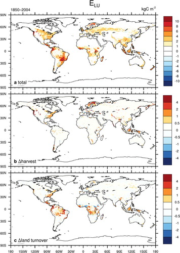
Fig. 4 Spatial distribution of cumulative historical (1850–2004) land use change (LUC) emissions and its components. (a) Total (gross, incl. wood harvest) cumulative LUC emissions in kgC/m². (b) Cumulative emissions due to wood harvest. (c) Effect of land turnover (including the introduction of secondary land) as the difference between the run with gross land use (LU) transitions and a run with net LU transitions; both runs do not consider wood harvest. Note the different colour scales in the upper and the lower two panels.

Simulated cumulative harvested biomass is 126 GtC for the period 1500–2004, somewhat below the number suggested by the LUH data (136 GtC, see also discussion in Section 4). Wood harvest is generally followed by re-growth, and the net effect on the terrestrial C balance is determined by changes in harvest intensity and extent. In our simulations, the effect of wood harvest on LU-related emissions is most pronounced in a few, mostly extra-tropical regions (Fig. 4b), but generally represents an additional source in all continents, although with differing trends in the source strength over the last decades. While the source has been steadily increasing in Latin America, it shows a slowly declining trend after 1980 in Europe, while the harvest source in Russia is recovering from a temporary, but large decrease in the 1990s.

We further distinguish different driving factors by quantifying primary emissions in direct response to LU area and management change from a simulation where CO₂ and climate are kept constant, and the indirect effects of changing CO₂ and climate in additional runs [Table 3, e.g. Strassmann et al. (2008)]. Primary emissions explain most but not all of the total LUC emission. The difference between C storage on natural and agricultural land tends to increase under rising CO₂ due to its fertilising effects on trees (‘woody thickening’) (Gitz and Ciais, 2003). In contrast, climate warming tends to reduce C storage due to faster soil decomposition and forest decline in some areas and generally reduces the difference between C storage on natural and agricultural land (Strassmann et al., 2008). In our simulations, these indirect effects amplify total emissions from 1850 to 2004. The contribution from CO₂ effects dominates those from climate (+12% versus −2%, see Table 3).

3.2. Projected emissions for the RCP scenarios

Total cumulative LUC emissions from 2005 to 2099 range between 27 and 151 GtC for the four RCPs (Table 4). Total LUC fluxes decrease to about 0.5 GtC/yr by 2100 in RCP 2.6 and RCP 6.0 and become negative in the second half of the century in RCP 4.5 (Fig. 5). In contrast, fluxes remain around current levels and are generally above 1 GtC/yr in RCP 8.5. Differences are due to different LU area and management trajectories but also due to different evolutions of CO₂ and climate. For the RCPs, we quantify the separate contribution of the combination of CO₂ and climate changes (Table 4).

Fig. 5 Annual land use change (LUC) fluxes for 1900–2100 and the different RCPs. Thick black and coloured curves are splined time series of annual data, which is shown by the thin solid curve for the past. Dashed and dotted lines represent annual LUC fluxes, diagnosed from a simulation without wood harvesting and from a simulation where only net LUC is simulated, respectively.

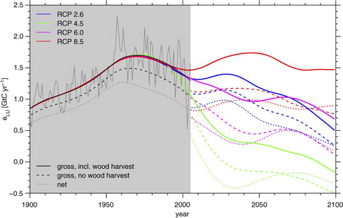
Fig. 6 Spatial distribution of cumulative future (RCPs) land use change (LUC) emissions and its components. Left: Total (gross, incl. wood harvest) cumulative LUC emissions in kgC/m² middle: Cumulative emissions due to wood harvest. Right: Effect of land turnover (including the introduction of secondary land) as the difference between the run with gross land use (LU) transitions and a run with net LU transitions; both runs do not consider wood harvest. Note the different colour scales in the panels.

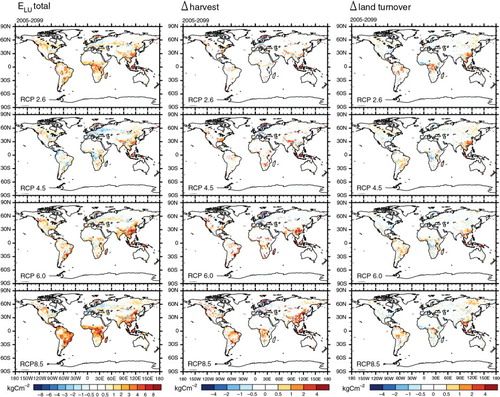
Table 4. Cumulative LUC emissions (E, [GtC]) for 2005–2099; combined effects from CO₂ and climate; and individual effects from wood harvest, and land turnover (shifting cultivation)

	RCP 2.6	RCP 4.5	RCP 6.0	RCP 8.5
Total	105	27	97	151
Primary	86	25	86	122
Climate & CO2	+19	+2	+12	+29
Harvest	+26	+37	+46	+53
Land turnover	+16	+13	+13	+13

Projected primary emissions due to direct changes in LU area and management are 25 GtC for RCP 4.5, and range between 86 and 122 GtC for the other RCPs (Table 4). The global cropland area, and to a lesser degree pasture areas, decreases in RCP 4.5 (Thomson et al., 2011) and, correspondingly, negative emissions from net LUC are simulated (see Fig. 5 and Fig. 6). These are compensated by impacts of shifting cultivation and wood harvest, finally leading to positive total emissions in spite of a contraction of areas under agricultural use. RCP 6.0 suggests an increase in croplands and a contraction in pasture areas (Masui et al., 2011). In our RCP 6.0 simulations, positive emissions from cropland expansion dominate over negative emissions from pasture contraction (38 GtC emissions from net LUC as a result of simultaneous pasture and cropland area changes). Emissions from continuously rising wood harvest in RCP 6.0 (46 GtC emission, see Table 4) add to that. RCP 8.5 and RCP 2.6 both feature an expansion of cropland areas (Riahi et al., 2011; van Vuuren et al., 2011b). This is driven by increasing population in RCP 8.5 and by expanding bio-energy production in RCP 2.6. However, these scenarios differ widely with respect to wood harvest, which causes a source of 26 GtC in RCP 2.6 and of 53 GtC in RCP 8.5. Land turnover (shifting cultivation) contributes about equally in all scenarios (13–16 GtC).

The combination of CO₂ and climate change increase the impact of LU in terms of net emissions (Table 4) in all RCPs and contribute between 8 and 19% to total cumulative LUC emissions. We did not quantify individual contributions from CO₂ and climate change for the future period.

In general, the contribution of wood harvest and shifting cultivation effects on total LUC emissions is considerable in recent decades. Under all RCP scenarios, additional emissions from effects of shifting cultivation remain important. Additional emissions from wood harvest increase throughout the 21st century to represent a major contribution to total LUC emissions by 2100. Emissions, particularly in RCP 6.0 and RCP 8.5, are underestimated in simulations only accounting for net LUCs and neglecting wood harvest.

3.3. Generated LU transitions

Total e_LU for LUH exhibits values of around 0.2–0.3 GtC yr⁻¹ during the first decades of the transient simulation (after 1500), declining thereafter (see Fig. 2). This variation is a simulation artefact and is not related to the rate of expansion of agricultural area, which increases by 0.12–0.19% yr⁻¹between 1500 and 1650 without any change in the long-term trend. This points to a shift in the mean C density of deforested land and is not attributable to changes in climate or CO₂ as the effect is seen also for primary emissions (not shown).

In the LUH data, secondary land is zero by design in 1500. In order to comply with land areas as defined in LUH, land abandonment during spin-up re-enters the ‘primary’ LU category. The secondary land area starts growing only after 1500. This shift is associated with a change in vegetation C density from areas claimed: 5.9 kgC/m² on primary land in 1500 (in grid cells with croplands present in 1500), declining to 5.7 kgC/m² on primary and 2.6 kgC/m² on secondary land in the same areas in 1650. e_LU is co-determined by the vegetation C density of deforested land. At the start of the simulation, land is only claimed from the primary LU class (secondary is zero), while at a later stage, land to be converted is (primarily) claimed from secondary land. The difference in vegetation C density on respective lands thus implies an agreeing shift in e_LU.

According to the argument outlined above, the initially anomalously high flux obtained with the LUH data hence arises from the idealised initialisation of LUH with no secondary land at 1500; we note that fluxes after around 1650 are hardly affected by this initialisation. The method described here as ‘GNT’ evades such a shift in transition priorities and mean C density as transition rules are fully maintained between spin-up and the transient simulation. Consequently, land claimed from secondary at 1500 is similar to 1650 and changes are only due to differences in land conversion rates. Also, the mean vegetation C density (on secondary land) shows no abrupt change with GNT (4.7 kgC/m² in 1500 vs. 5.6 kgC/m² in 1650). This implies stable e_LU after the spin-up and no anomalously high fluxes (artefact fluxes) occur (see Fig. 2).

In other words, the cumulative artefact flux in the simulations based on the LUH data is a delayed equilibration in response to changing transition patterns after the spinup, whereas transition patterns are consistent between the spinup and the transient simulation in the GNT approach, and C pool equilibration to the initial LU transition regime is fully realised already during spinup. It is noted, that cumulative pre-1850 emissions as reported above and in Table 3 are not affected by this issue. During the period 1850–2004, e_LU from GNT compares well with e_LU from LUH and generally deviates by less than 0.1 GtC yr⁻¹ (splined curve). Total cumulative LUC emissions between 1850 and 2004 are 165 GtC, 6 GtC less than in the simulations with prescribed LUH data.

4. Discussion

4.1. Past

The LPX-Bern 1.0, a DGVM simulating the coupled cycling of carbon and nitrogen, was applied to estimate carbon emissions from LU and LUC. Simulated cumulative historical (1850–2004) total emissions are 171 GtC (154 GtC primary emissions). This is within, but at the upper end of the range of previous studies (DeFries et al., 1999; Strassmann et al., 2008; Piao et al., 2009; Pongratz et al., 2009; Shevliakova et al., 2009; Van Minnen et al., 2009; Arora and Boer, 2010; Houghton, 2010; Reick et al., 2010); also for decadal mean emissions (Houghton et al., 2012; Le Quéré et al., 2013), here quantified at 1.55, 1.57, and 1.21 GtC/yr for the 1980s, 1990s and 2000–2004. In addition to emissions from net LUC, land turnover (shifting cultivation) and wood harvest have caused a cumulative historical (1850–2004) source of 25 and 23 GtC, respectively.

Primary emissions without shifting cultivation and wood harvest are 109 GtC. This value is a third lower than values reported by Stocker et al. (2011), who used an earlier version of LPX. This reduction is primarily due to the inclusion of C–N interactions and changed decomposition rates of soil carbon pools [as described in Spahni et al. (2013), Table 1] in the present study, which leads to a reduction of NPP and C pools on natural land particularly in the extra-tropics, where pools have been systematically overestimated in the previous version (Stocker et al., 2011). Higher emissions due to land turnover and forest management partially cancel the reduction associated with C–N interactions. Finally, pre-industrial primary emissions are only slightly higher than reported by Stocker et al. (2011).

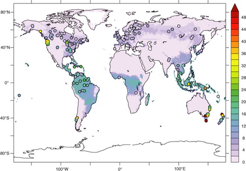
LUC emissions scale with the C density of deforested vegetation. LPX suggests a global total vegetation C stock of 492 GtC in 1500, declining to 324 GtC by 1990 and 318 GtC by 2000. This global number is good agreement with the global forest C stock estimate by Pan et al. (2011) of 367 GtC in 1990, dropping to 361 GtC in 2000. A comparison of model results with site-scale observations (Luyssaert et al., 2007; Keith et al., 2009) of forest C stock density is presented in Fig. 7 and suggests that also the spatial pattern of vegetation C density is well captured by the model.

Fig. 7 Simulated (map) and observational (dots) vegetation carbon density (kgC/m²). The map represents total vegetation C density in the primary land use class at present day, diagnosed from a simulation without any anthropogenic LUC and wood harvest. Observational data are from Luyssaert et al. (2007) and Keith et al. (2009) and also represent primary forests.

Additionally, the harvested forest area is determined by vegetation C density, as the LUH input data used here is given on a mass basis. Thus, inconsistencies may arise when the simulated total vegetation C is too small and cannot satisfy the required harvested mass in the respective grid cell, or when prescribed harvest-related wood extraction rates exceeds the simulated annual regrowth (sustainable yield). These effects explain the slight mismatch between prescribed harvest C mass (cumulatively 136 GtC) and the actually simulated harvested C mass (126 GtC). We assessed alternative implementations of wood harvest in the model. Using LUH harvest data on an area basis, where the harvested mass is ‘translated’ into areas by Hurtt et al. (2006) using their vegetation model, evades such effects but leads to lower cumulative wood harvest in combination with LPX (83 GtC, not shown) due to differences in simulated vegetation C density in the two models. However, effects of different implementations of wood harvesting on total LUC emissions are smaller and are in the order of ±5% of the numbers reported here.

Simulating past emissions relying on input information for gross LU transitions imposes technical challenges. Required information to define the full transition matrices is sparse and assumptions have to be made with respect to the turnover rate of agricultural land, priorities defining the LU category at which expense expansion in another or wood harvest is satisfied, and the spatio-temporal distribution of areas with significant land turnover (shifting cultivation). From our experience, processing pre-defined LU transition matrices, numerically consistent with pre-defined LU states, has proven technically costly and imposed a conceptual obstacle for model spin-up (see Section 3.3). A generic construction of the transition matrices based on LU states (see Section 2.2) is successful at relieving technical chalenges and realising C pool equilibration during model spin-up. Our results based on this GNT method are in good agreement with results using the full transition information from the LUH dataset. This thus demonstrates that the GNT method can be applied in combination with any existing LU reconstruction (Pongratz et al., 2009; Klein Goldewijk et al., 2011; Kaplan et al., 2011) and may be useful for Monte-Carlo type simulations with a probabilistic exploration of LU reconstruction uncertainties.

4.2. Future

The contribution of wood harvest to total LUC emissions is expected to increase under all future scenarios and should thus be accounted for in future estimates of LUC emissions. The contribution of total LUC-related CO₂ emissions to total CO₂ emissions in 2100, including emissions from fossil fuels, is expected to decrease to ~10% in the high-CO₂ scenario RCP 8.5 (Riahi et al., 2011), but makes up as much as ~30% in the strong mitigation scenario RCP 2.6 (van Vuuren et al., 2011b).

Only a few studies are available that addressed LUC emissions under future RCP scenarios (Hurtt et al., 2011; Lawrence et al., 2012; Brovkin et al., 2013). However, these report emissions from above-ground biomass (Hurtt et al., 2011), do not separate the LUC flux from other drivers (Lawrence et al., 2012), or do not separate effects of wood harvest and land turnover (Brovkin et al., 2013). This prevents a thorough comparison to results presented here. Brovkin et al. (2013) report cumulative RCP 2.6 emissions of 19–175 GtC and 25–205 GtC for RCP 8.5. Our results (105 GtC for RCP 2.6 and 151 GtC for RCP 8.5) fall inside these ranges. Among the models used in (Brovkin et al., 2013), MPI-ESM-LR suggests the largest emissions and respective values are closest to the ones presented here. Note, that this model also includes effects of wood harvest and land turnover.

Our emission estimates for the RCPs are compatible with, but generally higher than the values provided by the Integrated Assessment Models (Ciais et al., 2013). Simulated cumulative LUC emissions in RCP 4.5 and RCP 6.0 presented here differ most from those suggested by the IAMs. This is linked to different simulated impacts of conversion to and from croplands and pastures in the IAMs and LPX, as well as to differences in the simulated sensitivity of land C storage to CO₂ and climate and associated indirect emissions.

4.3. System boundaries

Emissions presented here include effects from deforestation and shifting cultivation, legacy fluxes, decay of wood products, lost sinks/sources under changing environmental conditions, and wood and crop harvest both for the past and the future. Simulated emissions do not include contributions from peat burning or degradation, anthropogenic fire suppression, and anthropogenically induced fires not aimed at cropland or pasture expansion. Effects of accelerated soil turnover due to tillage and crop harvest are simulated here and lead to higher emissions compared to, for example, Pongratz et al. (2009).

Deforestation due to land conversion is not counted towards fulfilling harvest statistics. This may bias simulated emissions towards high values. We assessed this effect in separate simulations by using deforested (felled) biomass of cropland and pasture expansion to satisfy wood harvest in the respective grid cell (not shown). However, the effect on total LUC emissions is small (−1.8%, mean over 1980–2004), partly because of the spatial mismatch between areas of agricultural expansion and areas with substantial wood harvesting.

A further aspect that may bias LUC emissions high is that open grasslands are not preferentially claimed for pasture expansion. Here, transitions between LU categories are independent of the dynamically simulated vegetation distribution. This guarantees consistency with the original LUH data and is in contrast to the approach followed by Reick et al. (2013) where transitions are formulated with respect to the vegetation cover area.

The LUH data are based on the HYDE reconstruction (Klein Goldewijk et al., 2011), where a constant per-capita land requirement is assumed to back-project LU areas before census data became available. Kaplan et al. (2011) argue that per-capita land requirements were higher at earlier times, but their LU data do not cover the period after 1850. The use of the LUH data likely leads to a low bias in pre-industrial emissions and a correspondingly high bias in emissions during later periods as any LU history has to converge to the current LU distribution.

Our results rely on simulations with prescribed observed atmospheric CO₂ (and climate) in both simulations with and without LUC. This ignores the fact that observational CO₂ (and climate) carry the signal of actual historical LUC, which stimulated terrestrial C uptake. This negative flux termed ‘LU feedback’ by Strassmann et al. (2008) should be assigned to LUC emissions, but is not included here. This issue is common to all DGVM-based LUC estimates relying on results from simulations with prescribed CO₂ and climate. Total LUC fluxes/emissions reported here correspond to method D3 described in Pongratz et al. (2014), while primary LUC fluxes/emissions correspond to method D1.

5. Conclusion

Global vegetation models simulating the full complexity of LUC, with wood harvesting and parallel expansion and abandonment of agricultural land, consistently suggest higher LUC C emissions (Shevliakova et al., 2009; Brovkin et al., 2013) than ‘traditional’ models accounting only for net LUC. Here, we quantified the additional source of wood harvest and land turnover each at 0.23 GtC/yr, or 19% of total LUC emissions in the 2000s – a relatively large contribution that is expected to remain high or increase under all future RCP scenarios. Higher emission estimates from LUC imply a larger residual terrestrial C sink to comply with global C budget constraints for the last decades.

However, the implementation of gross LUC in models imposes technical challenges and relies on extensive information as input, often unavailable for different scenarios of historical LUC. We presented a method to reduce these obstacles by generically generating transition matrices and demonstrated its potential applicability to any dataset defining only net LUC.

6. Acknowledgements

This study received support from the Swiss National Science Foundation through the NCCR Climate and the Sinergia project iTree as well as by the European Commission through the FP7 projects Past 4 Future (grant no. 243908).

7. Appendix

A conversion of LU areas

This section describes the conversion of soil, vegetation, litter, and product carbon pools. In any grid cell, the soil C content associated with a LU category k is , where is the soil C density. For LU transitions between time t and t+1, s _k is updated as:A1

where l runs over all LU categories. Thus, soil C is re-averaged over the changed LU areas. For vegetation C, is the mass per plant individual of PFT i. Vegetation C is removed from converted areas. For grasses and mosses, LU transitions are modelled as:A2

where ζ _ik is one if PFT i is in LU category k and zero otherwise. For trees, the vegetation C content per individual is unaffected by LUC but the density of individuals N _i is modified:A3

Removed vegetation enters litter and product pools. Litter is associated with the PFT of the plant it derives from, while products are associated with LU categories. Distribution of fresh litter, along with the redistribution of old litter is calculated as:A4

where is one if PFTs and j are ‘related’, meaning biologically identical PFTs associated to different LU categories. For unrelated PFT pairs, ρ _ij is zero. The right hand side terms of eq. (A4) describe, from left to right, change of litter content in analogy to eqs. (A2) and (A3), litter and vegetation input from related PFTs, and litter input from unrelated PFTs. The latter is distributed among all the PFTs of the respective LU category (N _PFT,K is the number of PFTs in k).

Equation (A4) applies to leaf and root plant parts, while heartwood and sapwood is not transferred to litter pools but to product pools. Product pools only exist for the LU categories primary and secondary natural land. Carbon entering a product pool is not affected by any further LU transitions and is released to the atmosphere according to product pool-specific decay times (0, 2, and 20 yr). The fractional distribution to the different product pools depends on the origin of the wood.

References

- Arora V. K , Boer G. J . Uncertainties in the 20th century carbon budget associated with land use change. Glob. Change Biol. 2010; 16(12): 3327–3348.
- Baccini A , Goetz S. J , Walker W. S , Laporte N. T , Sun M , co-authors . Estimated carbon dioxide emissions from tropical deforestation improved by carbon-density maps. Nat. Clim. Change. 2012; 2: 182–185.
- Bala G , Caldeira K , Wickett M , Phillips T. J , Lobell D. B , co-authors . Combined climate and carbon-cycle effects of large-scale deforestation. Proc. Natl. Acad. Sci. U. S. A. 2007; 104(16): 6550–6555. [PubMed Abstract] [PubMed CentralFull Text].
- Brovkin V , Boysen L , Arora V. K , Boisier J. P , Cadule P , co-authors . Effect of anthropogenic land-use and land-cover changes on climate and land carbon storage in CMIP5 projections for the twenty-first century. J. Clim. 2013; 26(18): 6859–6881.
- Ciais P , Sabine C , Bala G , Bopp L , Brovkin V , co-authors . Chapter 6: carbon and other biogeochemical cycles. Climate Change 2013: The Physical Science Basis. Working Group I Contribution to the Fifth Assessment Report of the Intergovernmental Panel on Climate Change. 2013. Final Draft, 7 June 2013.
- Claussen M , Brovkin V , Ganopolski A . Biogeophysical versus biogeochemical feedbacks on large-scale land cover change. Geophys. Res. Lett. 2001; 28: 1011–1014.
- Davidson E. A , Ackerman I. L . Changes in soil carbon inventories following cultivation of previously untilled soils. Biogeochemistry. 1993; 20(3): 161–193.
- DeFries R. S , Field C. B , Fung I , Collatz G. J , Bounoua L . Combining satellite data and biogeochemical models to estimate global effects of human-induced land cover change on carbon emissions and primary productivity. Glob. Biogeochem. Cycles. 1999; 13: 803–815.
- Dufresne J.-L , Foujols M.-A , Denvil S , Caubel A , Marti O , co-authors . Climate change projections using the IPSL-CM5 earth system model: from CMIP3 to CMIP5. Clim. Dyn. 2013; 40(9–10, SI): 2123–2165.
- Feddema J. J , Oleson K. W , Bonan G. B , Mearns L. O , Buja L. E , co-authors . The importance of land-cover change in simulating future climates. Science. 2005; 310(5754): 1674–1678. [PubMed Abstract].
- Gaillard M.-J , Sugita S , Mazier F , Trondman A.-K , Broström A , co-authors . Holocene land-cover reconstructions for studies on land cover-climate feedbacks. Clim. Past. 2010; 6(4): 483–499.
- Gitz V , Ciais P . Amplifying effects of land-use change on future atmospheric CO2 levels. Glob. Biogeochem. Cycles. 2003; 17: 1024.
- Guo L. B , Gifford R. M . Soil carbon stocks and land use change: a meta analysis. Glob. Change Biol. 2002; 8: 345–360.
- Harris N. L , Brown S , Hagen S. C , Saatchi S. S , Petrova S , co-authors . Baseline map of carbon emissions from deforestation in tropical regions. Science. 2012; 336(6088): 1573–1576. [PubMed Abstract].
- Houghton R. A . The annual net flux of carbon to the atmosphere from changes in land use 1850–1990. Tellus B. 1999; 51: 298–313.
- Houghton R. A . How well do we know the flux of CO2 from land-use change. Tellus B. 2010; 62: 337–351.
- Houghton R. A , Hobbie J. E , Melillo J. M , Moore B , Peterson B. J , co-authors . Changes in the carbon content of terrestrial biota and soils between 1860 and 1980 – a net release of CO2 to the atmosphere. Ecol. Monogr. 1983; 53: 235–262.
- Houghton R. A , House J. I , Pongratz J , van der Werf G. R , DeFries R. S , co-authors . Carbon emissions from land use and land-cover change. Biogeosciences. 2012; 9(12): 5125–5142.
- Hurtt G. C , Chini L. P , Frolking S , Betts R. A , Feddema J , co-authors . Harmonization of land-use scenarios for the period 1500–2100: 600 years of global gridded annual land-use transitions, wood harvest, and resulting secondary lands. Clim. Change. 2011; 109: 117–161.
- Hurtt G. C , Frolking S , Fearon M. G , Moore B , Shevliakova E , co-authors . The underpinnings of land-use history: three centuries of global gridded land-use transitions, wood-harvest activity, and resulting secondary lands. Glob. Change Biol. 2006; 12: 1208–1229.
- IUCN. IUCN Red List of Threatened Species. 2000; Gland, Switzerland: The World Conservation Union.
- Kaplan J. O , Krumhardt K. M , Ellis E. C , Ruddiman W. F , Lemmen C , co-authors . Holocene carbon emissions as a result of anthropogenic land cover change. Holocene. 2011; 21(5): 775–791.
- Keith H , Mackey B. G , Lindenmayer D. B . Re-evaluation of forest biomass carbon stocks and lessons from the world's most carbon-dense forests. Proc. Natl. Acad. Sci. U. S. A. 2009; 106(28): 11635–11640. [PubMed Abstract] [PubMed CentralFull Text].
- Klein Goldewijk K , Beusen A , van Drecht G , de Vos M . The HYDE 3.1 spatially explicit database of human-induced global land-use change over the past 12,000 years. Glob. Ecol. Biogeogr. 2011; 20(1): 73–86.
- Lamarque J.-F , Kyle G. P , Meinshausen M , Riahi K , Smith S. J , co-authors . Global and regional evolution of short-lived radiatively-active gases and aerosols in the representative concentration pathways. Clim. Change. 2011; 109(1–2, SI): 191–212.
- Lawrence P. J , Feddema J. J , Bonan G. B , Meehl G. A , O'Neill B. C , co-authors . Simulating the biogeochemical and biogeophysical impacts of transient land cover change and wood harvest in the Community Climate System Model (CCSM4) from 1850 to 2100. J. Clim. 2012; 25(9): 3071–3095.
- Le Quéré C , Andres R. J , Boden T , Conway T , Houghton R. A , co-authors . The global carbon budget 1959–2011. Earth Syst. Sci. Data. 2013; 5(1): 165–185.
- Luyssaert S , Inglima I , Jung M , Richardson A. D , Reichstein M , co-authors . CO2 balance of boreal, temperate, and tropical forests derived from a global database. Glob. Change Biol. 2007; 13(12): 2509–2537.
- MacFarling Meure C , Etheridge D , Trudinger C , Steele P , Langenfelds R , co-authors . Law Dome CO(2), CH(4) and N(2)O ice core records extended to 2000 years BP. Geophys. Res. Lett. 2006; 33: L14810.
- Masui T , Matsumoto K , Hijioka Y , Kinoshita T , Nozawa T , co-authors . An emission pathway for stabilization at 6 Wm(-2) radiative forcing. Clim. Change. 2011; 109(1–2, SI): 59–76.
- McGuire A. D , Sitch S , Clein J. S , Dargaville R , Esser G , co-authors . Carbon balance of the terrestrial biosphere in the twentieth century: analyses of CO2, climate and land use effects with four process-based ecosystem models. Glob. Biogeochem. Cycles. 2001; 15: 183–206.
- Mitchell T. D , Jones P. D . An improved method of constructing a database of monthly climate observations and associated high-resolution grids. Int. J. Climatol. 2005; 25(6): 693–712.
- Murty D , Kirschbaum M , Mcmurtrie R , Mcgilvray H . Does conversion of forest to agricultural land change soil carbon and nitrogen? A review of the literature. Glob. Change Biol. 2002; 8: 105–123.
- Ogle S. M , Breidt F. J , Paustian K . Agricultural management impacts on soil organic carbon storage under moist and dry climatic conditions of temperate and tropical regions. Biogeochemistry. 2005; 72: 87–121.
- Olofsson J , Hickler T . Effects of human land-use on the global carbon cycle during the last 6,000 years. Veg. Hist. Archaeobot. 2008; 17(5): 605–615.
- Pan Y , Birdsey R. A , Fang J , Houghton R , Kauppi P. E , co-authors . A large and persistent carbon sink in the world's forests. Science. 2011; 333(6045): 988–993. [PubMed Abstract].
- Piao S , Ciais P , Friedlingstein P , de Noblet-Ducoudré N , Cadule P , co-authors . Glob. Biogeochem. Cycles. 2009; 23: GB4026. Spatiotemporal patterns of terrestrial carbon cycle during the 20th century DOI: 10.1029/2008GB003339.
- Pongratz J , Reick C , Raddatz T , Claussen M . A reconstruction of global agricultural areas and land cover for the last millennium. Glob. Biogeochem. Cycles. 2008; 22(3): B3018+.
- Pongratz J , Reick C. H , Houghton R. A , House J. I . Terminology as a key uncertainty in net land use and land cover change carbon flux estimates. Earth Syst. Dyn. 2014; 5(1): 177–195.
- Pongratz J , Reick C. H , Raddatz T , Claussen M . Effects of anthropogenic land cover change on the carbon cycle of the last millennium. Glob. Biogeochem. Cycles. 2009; 23(4): B4001+.
- Ramankutty N , Foley J. A . Estimating historical changes in global land cover: croplands from 1700 to 1992. Glob. Biogeochem. Cycles. 1999; 13: 997–1027.
- RCP Database. RCP database, version 2.0.5. 2009. Online at: http://www.iiasa.ac.at/web-apps/tnt/RcpDb/ [Accessed 27 October 2011]..
- Reick C. H , Raddatz T , Brovkin V , Gayler V . Representation of natural and anthropogenic land cover change in MPI-ESM. J. Adv. Model. Earth Syst. 2013. 5(3), 459–482.
- Reick C. H , Raddatz T , Pongratz J , Claussen M . Contribution of anthropogenic land cover change emissions to pre-industrial atmospheric CO2. Tellus B. 2010; 62(5, SI): 329–336.
- Riahi K , Rao S , Krey V , Cho C , Chirkov V , co-authors . RCP 8.5-A scenario of comparatively high greenhouse gas emissions. Clim. Change. 2011; 109(1–2, SI): 33–57.
- Shevliakova E , Pacala S. W , Malyshev S , Hurtt G. C , Milly P. C. D , co-authors . Carbon cycling under 300 years of land use change: importance of the secondary vegetation sink. Glob. Biogeochem. Cycles. 2009; 23(2): 2022.
- Sitch S , Smith B , Prentice I. C , Arneth A , Bondeau A , co-authors . Evaluation of ecosystem dynamics, plant geography and terrestrial carbon cycling in the LPJ dynamic global vegetation model. Glob. Change Biol. 2003; 9: 161–185.
- Spahni R , Joos F , Stocker B. D , Steinacher M , Yu Z. C . Transient simulations of the carbon and nitrogen dynamics in northern peatlands: from the last glacial maximum to the 21st century. Clim. Past. 2013; 9(3): 1287–1308.
- Stocker B. D , Roth R , Joos F , Spahni R , Steinacher M , co-authors . Multiple greenhouse-gas feedbacks from the land biosphere under future climate change scenarios. Nat. Clim. Change. 2013; 3(7): 666–672.
- Stocker B. D , Strassmann K , Joos F . Sensitivity of holocene atmospheric CO2 and the modern carbon budget to early human land use: analyses with a process-based model. Biogeosciences. 2011; 8(1): 69–88.
- Strassmann K. M , Joos F , Fischer G . Simulating effects of land use changes on carbon fluxes: past contributions to atmospheric CO2 increases and future commitments due to losses of terrestrial sink capacity. Tellus B. 2008; 60(4): 583–603.
- Taylor K. E , Stouffer R. J , Meehl G. A . An overview of CMIP5 and the experiment design. Bull. Am. Meteorol. Soc. 2012; 93(4): 485–498.
- Thomson A. M , Calvin K. V , Smith S. J , Kyle G. P , Volke A , co-authors . RCP4.5: a pathway for stabilization of radiative forcing by 2100. Clim. Change. 2011; 109(1–2, SI): 77–94.
- UNEP. Global Environmental Outlook-3: Past, Present, and Future Perspectives. 2002; Nairobi, Kenya: United Nations Environment Programme.
- Van Minnen J. G , Goldewijk K. K , Stehfest E , Eickhout B , van Drecht G , co-authors . The importance of three centuries of land-use change for the global and regional terrestrial carbon cycle. Clim. Change. 2009; 97(1–2): 123–144.
- van Vuuren D. P , Edmonds J , Kainuma M , Riahi K , Thomson A , co-authors . The representative concentration pathways: an overview. Clim. Change. 2011a; 109(1–2, SI): 5–31.
- van Vuuren D. P , Stehfest E , den Elzen M. G. J , Kram T , van Vliet J , co-authors . RCP2.6: exploring the possibility to keep global mean temperature increase below 2°C. Clim. Change. 2011b; 109(1–2, SI): 95–116.
- Watson R. T , Noble I. R , Bolin B , Ravindranath N. H , Verardo D. J , co-authors . Land use, land-use change and forestry. Climate Change 2013: The Physical Science Basis. Working Group I Contribution to the Fifth Assessment Report of the Intergovernmental Panel on Climate Change. 2000. Final Draft, 7 June 2013.
- Xu-Ri Prentice I. C . Terrestrial nitrogen cycle simulation with a dynamic global vegetation model. Glob. Change Biol. 2008; 14(8): 1745–1764.
- Zaehle S , Ciais P , Friend A. D , Prieur V . Carbon benefits of anthropogenic reactive nitrogen offset by nitrous oxide emissions. Nat. Geoscience. 2011; 4(9): 601–605.