Close relationship between spectral vegetation indices and V_cmax in deciduous and mixed forests

Abstract

Seasonal variations of photosynthetic capacity parameters, notably the maximum carboxylation rate, V_cmax, play an important role in accurate estimation of CO₂ assimilation in gas-exchange models. Satellite-derived normalised difference vegetation index (NDVI), enhanced vegetation index (EVI) and model-data fusion can provide means to predict seasonal variation in V_cmax. In this study, V_cmax was obtained from a process-based model inversion, based on an ensemble Kalman filter (EnKF), and gross primary productivity, and sensible and latent heat fluxes measured using eddy covariance technique at two deciduous broadleaf forest sites and a mixed forest site. Optimised V_cmax showed considerable seasonal and inter-annual variations in both mixed and deciduous forest ecosystems. There was noticeable seasonal hysteresis in V_cmax in relation to EVI and NDVI from 8 d composites of satellite data during the growing period. When the growing period was phenologically divided into two phases (increasing VIs and decreasing VIs phases), significant seasonal correlations were found between V_cmax and VIs, mostly showing R²>0.95. V_cmax varied exponentially with increasing VIs during the first phase (increasing VIs), but second and third-order polynomials provided the best fits of V_cmax to VIs in the second phase (decreasing VIs). The relationships between NDVI and EVI with V_cmax were different. Further efforts are needed to investigate V_cmax–VIs relationships at more ecosystem sites to the use of satellite-based VIs for estimating V_cmax.

• V_cmax
• spectral vegetation indices
• ensemble Kalman filter
• BEPS model

1. Introduction

Carbon, water and energy exchanges between ecosystems and the atmosphere play an important role in the earth's climate. Terrestrial ecosystem models are important tools for understanding and simulating the behaviour of land ecosystems and their responses to various disturbances (Lu et al., 2013). Photosynthesis, one of the major components of the terrestrial carbon cycle, is a crucial factor in an ecosystem carbon cycle (Field et al., 1995; Sellers et al., 1997). In applications of Farquhar's model (Farquhar et al., 1980; Chen et al., 1999; Kimball et al., 2000), the saturated or maximum rate of Rubisco carboxylation, V_cmax, has been generally accepted as the measure of photosynthetic capacity, which is a pivotal parameter in models simulating photosynthesis. Evidence increasingly indicates that large seasonal and inter-annual variations in V_cmax occur in terrestrial ecosystems, especially in deciduous forests (Wilson et al., 2000; Xu and Baldocchi, 2003; Wang et al., 2008b). In most models, however, V_cmax has simply been assumed to be a constant, specific only to vegetation types, without seasonal variation (Stickan et al., 1994; Vonstamm, 1994; Bonan, 1995; Hoffmann, 1995). Ignoring seasonal variation in V_cmax in models can result in a large deviation in simulated carbon uptake (Tu, 2000; Wilson et al., 2001; Kosugi et al., 2003; Wang et al., 2004b).

The traditional way to obtain V_cmax is from direct gas-exchange measurements on leaves, branches or whole plants in specially designed cuvettes (Xu and Baldocchi, 2003; Grassi et al., 2005; Misson et al., 2006; Fan et al., 2011). However, direct measurements are not operational in spatial or long-term applications due to the intensive labour and time requirements of the work. The model-data fusion technique can provide an effective way to optimise seasonality in V_cmax. Wang et al. (2004a) proposed an alternative approach to determine V_cmax seasonality by inverting a detailed process-based model. Wang et al. (2007) estimated V_cmax in a land surface model by applying nonlinear inversion technique to eddy covariance (EC) measurements of gross primary photosynthesis (GPP). Santaren et al. (2007) have shown that model parameters related to photosynthesis were well resolved by EC-measured GPP. Mo et al. (2008), using EC measurements, found that data assimilation using an ensemble Kalman filter (EnKF) can successfully track the seasonal and inter-annual variation in parameters related to photosynthesis. Ju et al. (2010) also found that site-specific V_cmax could be optimised well by using EC-measured carbon and water fluxes and EnKF. However, using site-specific static parameter values may not lead to accurate estimation of regional-scale C fluxes (Wang et al., 2007). Therefore, a simpler alternative method capable of describing seasonal variations in V_cmax is needed for improving the estimation of regional carbon fluxes.

Canopy and leaf properties obtained through multispectral digital imaging at different spatial and temporal scales provide an effective way to obtain photosynthetic capacity. Leaf pigments link photosynthesis to leaf spectral properties and absorbed photosynthetically active radiation. Accurate leaf pigment content can be acquired from leaf reflectance spectra in visible and near infrared regions (Gamon and Surfus, 1999; Gitelson et al., 2009). Research has shown that remotely sensed reflectance can provide a useful data source to sense photosynthetic capacity because of the linkage of reflectance with canopy photosynthesis (Gamon et al., 1995; Carter, 1998; Choudhury, 2001; Dobrowski et al., 2005). A variety of vegetation indices have been used that can be related to photosynthetic capacity, notably the normalised difference vegetation index (NDVI), and the enhanced vegetation index (EVI) (Wang et al., 2009; Jin et al., 2012; Muraoka et al., 2012; Houborg et al., 2013).

In spite of broad acceptance that vegetation indices (VIs) can potentially track seasonal variation in photosynthetic capacity, there are few studies that directly demonstrate the correlation between V_cmax and various VIs. Studies by Wang et al. (2008a, 2009) and Jin et al. (2012) revealed noticeable inconsistencies in the relationship between V_cmax and VIs in certain periods, for example, V_cmax increasing with increasing VIs in spring and then decreasing or remaining steady with further increase of VIs. Stronger relationships might be obtained by allowing for hysteresis or asymmetric V_cmax–VI relationships. Muraoka et al. (2012) found better relationships between V_cmax and LAI for a deciduous broadleaf forest by splitting the growing period into two phases. But, these relationships that exclude the inherent correlation between LAI and VIs need further investigation.

In this study, V_cmax was optimised using the process-based Boreal Ecosystem Productivity Simulator (BEPS) model with an EnKF and using EC-measured GPP, latent heat (LE) and sensible heat (SH) fluxes in two broadleaf forest stands and one mixed forest stand. These V_cmax values were then related to NDVI and EVI. The main objectives of this investigation were to: (1) study seasonal and inter-annual variations in V_cmax in deciduous and mixed forests; and (2) analyse the correlation between V_cmax and VIs and, more importantly, the seasonal V_cmax–VIs relationships.

2. Materials and methods

2.1. Site description

Three forest FLUXNET sites are located in temperate climates at mid-latitudes, two with deciduous broadleaf stands and one with a mixed forest stand, were selected for this study. These were a mixed forest ecosystem at the Changbai Mountain Station site (CBS) in China, and two deciduous broadleaf forest ecosystems, an old aspen (SKOA) stand at the Prince Albert National Park, Canada, and the University of Michigan Biological Station site (UMBS), USA. Details of site information are listed in Table 1.

Table 1. Site description including name and location (latitude and longitude), canopy height, duration of measurements, stand age, dominant species composition, and references for each flux site in this study

Site	Country	Latitude, longitude	Canopy height (m)	Time span	Stand age (years)	Dominant species composition	References
CBS	China	42°24′9″N, 128°05′45″E	26	2003–2005	200	Pinus koraiensis, Tilia amurensis, Acer mono, Fraxinus mandshurica, Quercus mongolica	Yu et al., 2008; Zhang et al., 2009
SKOA	Canada	53°37′12″N, 106°11′24″W	23	2000–2002	74	Trembling aspen, Populus tremuloides Michx.	Gower et al., 1997; Krishnan et al., 2006; Mo et al., 2008
UMBS	America	45°33′35″N, 84°42′50″W	22	2000–2002	90	Populus grandidentata Michx., Quercus rubra L. Fagus grandifolia Ehrh., Acer rubrum L. and Pinus strobus L.	Curtis et al., 2005; Gough et al., 2013

The CBS site (42°24′9″N, 128°05′45″E) is located at the Changbai Mountain, northern China, which is influenced by the monsoons and typical characteristics of mid-latitudinal upland climate. Annual mean temperature is 0.9–4.0°C, and annual mean precipitation is 600–810 mm (evaluated over a period of 20 yr). The area is covered by a 200-yr-old, multistoried, uneven-aged, multispecies mixed forest consisting of mainly Korean pine (Pinus koraiensis), Tilia amurensis, Acer mono, Fraxinus mandshurica, Quercus mongolica and 135 other species (Yu et al., 2008; Zhang et al., 2009). The SKOA site (53°37′12″N, 106°11′24″W) is located in Prince Albert National Park, Saskatchewan, Canada, at an altitude of approximately 600 m. Flux measurements have continued there since 1994. The mean annual air temperature at SKOA is 0.4°C, and annual precipitation is 467 mm (Gower et al., 1997). The dominant tree species at this 73-yr-old 22 m high (in 2000) stand is trembling aspen (Populus tremuloides Michx.) (Krishnan et al., 2006; Mo et al., 2008). The UMBS site (45°33′35″N, 84°42′50″W) is located in the transition zone between mixed hardwood and boreal forests in northern lower Michigan, USA. Within a 1 km radius of the meteorological tower the forest is a secondary successional mixed northern hardwood forest. Dominant species consist of bigtooth aspen (Populus grandidentata Michx.), northern red oak (Quercus rubra L.), American beech (Fagus grandifolia Ehrh.), red maple (Acer rubrum L.) and white pine (Pinus strobus L.) (Gough et al., 2013). Canopy height is approximately 22 m with average tree age of 90 yr (in 2013). Mean annual temperature (1942–2003) is 5.5°C, and mean annual precipitation is 817 mm (Curtis et al., 2005).

2.2. Data sources

Meteorological and flux data used were taken from ChinaFLUX for CBS and from global FLUXNET database (http://fluxnet.ornl.gov/) for the other two sites. Measurements taken from January 1, 2003, to December 31, 2005, at CBS, January 1, 2000, to December 31, 2002, at SKOA, and January 1, 2000, to December 31, 2002, at UMBS were used. This encompassed a 2-yr (2001–2002) drought period at SKOA, and 2-yr (2001–2002) period of low temperatures at UMBS, thereby allowing the investigation of VIs versus V_cmax relationships under these abnormal climate conditions.

2.2.1. Meteorological data

The half-hourly meteorological data, including incoming solar radiation, air temperature, relative humidity, wind speed, and precipitation were used to drive the BEPS model. Gaps in meteorological data were filled in the following way: short gaps up to three hours were filled with linear interpolation; gaps up to 4 d were filled with average values at particular times of the day in a 14 d moving time window around the gap as explained in Falge et al. (2001a). Larger than 4 d gaps were filled with respective values averaged over the available time series following the procedure of Horn and Schulz (2011).

2.2.2. Flux data

EC measurements of GPP, SH and LE (half-hourly values) were used for parameter optimisation. Missing data in the time series of SH and LE were gap filled with look-up tables (LookUp) as defined in Falge et al. (2001b). GPP was calculated from the measured net ecosystem production (NEP) as follows: ecosystem respiration (Re) was calculated using the Lloyd & Taylor relationship (Lloyd and Taylor, 1994) between night-time NEP and soil temperature under turbulent conditions, and the GPP was calculated as the sum of daytime NEP and Re (Desai et al., 2008).

2.2.3. MODIS data

Composite 8 d MODIS reflectance products (MOD09A1 V05) at 500 m spatial resolution were used to analyse the seasonal and inter-annual variations in NDVI and EVI for the three sites. NDVI and EVI were calculated as: where ρ _nir , ρ _red , and ρ _blue are reflectance in the near infrared, red and blue band, respectively.

Calculated NDVI and EVI were further smoothed using a locally adjusted cubic-spline capping (LACC) method (Chen et al., 2006) to remove unrealistic fluctuations caused by residual cloud contamination and atmospheric noise.

2.3. BEPS model

Originating from the FOREST-BGC model (Running and Coughlan, 1988), the BEPS model (Chen et al., 1999) is a process-based model that includes energy partitioning, photosynthesis, autotrophic respiration, soil organic matter (SOM) decomposition, hydrological processes and soil heat transfer modules. In the model, GPP was the total net photosynthesis rates of sunlit and shaded leaves, calculated using the leaf level Farquhar model (Farquhar et al., 1980). The simulation of net photosynthesis rates of the sunlit and shaded leaves is coupled to leaf stomatal conductance by the Ball–Woodrow–Berry model (Ball et al., 1987). BEPS has been successfully used to estimate carbon and water fluxes regionally and globally (Grant et al., 2006; Chen et al., 2012; Schaefer et al., 2012), and also to optimise seasonal variations in photosynthetic parameters, including V_cmax for a subtropical evergreen coniferous plantation (Ju et al., 2010) and broadleaf forest (Mo et al., 2008). Details about the model are described in Ju et al. (2006).

Model input data include atmospheric variables, such as temperature, precipitation, wind spend, relative humidity, solar irradiance, vegetation type, stand age, canopy clumping index, texture and physical properties of soil. The model outputs include GPP, NEP, autotrophic and heterotrophic respiration, net radiation, LE and SH, soil moisture and temperature profiles. The simulation time step was set at 30 min.

2.4. Parameter optimisation

Model parameter optimisation was implemented using a dual state-parameter estimation method based on the EnKF (Reichstein et al., 2003; Aalto et al., 2004; Moradkhani et al., 2005; Mo et al., 2008; Ju et al., 2010). The parameter ensembles are updated as:where is the updated parameter ensemble at time step t+1; the parameter sample generated with an assumption that model parameters follow a random walk in prescribed space (Moradkhani et al., 2005); is the Kalman gain matrix for correcting parameter trajectories; and and are the ensemble members of observations and predictions, respectively.

Parameter sample is taken as:In eq. (3), the Kalman gain matrix is calculated as:where is the cross covariance between parameter ensemble and prediction ensemble; is the error covariance matrix of the prediction ; and is the error covariance of observation.

2.5. Parameters optimised and ensemble

The sensitivity analysis showed that four parameters, namely, V_cmax, J_max (i.e., electron transport capacity), the slope in the modified Ball–Berry model (M) and the coefficient determining the sensitivity of stomatal conductance to atmospheric water vapour deficit (D₀) had significant impacts on simulated GPP, LE and SH. As J_max could be calculated from V_cmax in the BEPS model (Chen et al., 1999), we optimised V_cmax, M and D₀ in this study. The ranges and standard deviations of these parameters are listed in Table 2. Estimation of observational errors is important in EnKF data assimilation because the observational errors determine the degree to which the parameters and simulations are to be corrected (Mo et al., 2008).

Table 2. Standard deviations and ranges of model parameters optimised

Symbol	Unit	Standard deviation	Range
Vcmax	µmol m^−2 s^−1	4	8–60
M	Dimensionless	0.8	2–16
D0	kPa	0.15	1.1–2.2

Furthermore, earlier studies have shown that observational errors in flux data are correlated to flux magnitudes (Lasslop et al., 2008; Richardson et al., 2008). While Elbers et al. (2011) found that the uncertainty of measured NEP of a mid-latitude temperate pine forest was about 8%. Goulden et al. (1996) found that in the Harvard Forest Monte Carlo simulations and the surface energy budget indicated a uniform systematic error of −20 to 0%. Typically, the overall accuracy of EC fluxes is in the range of 10–20% (Wesely and Hart, 1985; Santaren et al., 2007). Based on these studies, we set the uncertainties in half-hourly values of measured GPP, LE and SH at 10% and assumed these to be independent of one another. Also, Mo et al. (2008) found that when the ensemble size was larger than 100, the predicted fluxes were quite similar and the updated parameters reached approximately stable values. Thus, an ensemble size of 200 was used in this study. The three parameters were optimised when measured GPP, LE and SH were available and updated by applying cumulative corrections. Updated parameters were used to simulate fluxes at half-hourly time steps for the following days until the next parameter optimisation was conducted.

3. Results

3.1. Seasonal variation of environmental variables

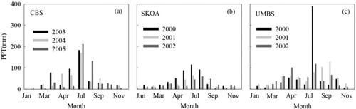
Average 8 d air temperature, T_a, cumulative 8 d solar radiation, S_w, and 8 d average vapour pressure deficit, VPD, during the measurement period at the three sites are displayed in Fig. 1, and monthly cumulative precipitation (PPT) is shown in Fig. 2. T_a showed typical seasonal variation with maximums in August and minimums in January at all three sites. SKOA and UMBS depicted stronger solar irradiance than that at CBS, where S_w increased slowly during January and April, stayed relatively steady during April to August, and finally decreased slowly to the end of the year. At SKOA and UMBS, S_w increased rapidly to maximum values in July and August, and then decreased rapidly towards the end of the year. While VPD at CBS was the highest in May and much lower during the rest of growing season, it remained high from the beginning of May to the end of August at SKOA and UMBS. Seasonal variation in T_a tended to match the trend in precipitation at CBS during 2003–2005 and at SKOA in 2000. In contrast, there were droughts in the summer of 2001 and 2002 at SKOA. At UMBS, precipitation was almost uniformly distributed from April to November except for very high precipitation in August of 2000.

Fig. 1 The seasonal variations in 8 d average air temperature, T_a (a–c), cumulative 8 d solar radiation, S_w (d–f), and 8 d average vapour pressure deficit, VPD (g–i), for CBS, SKOA and UMBS.

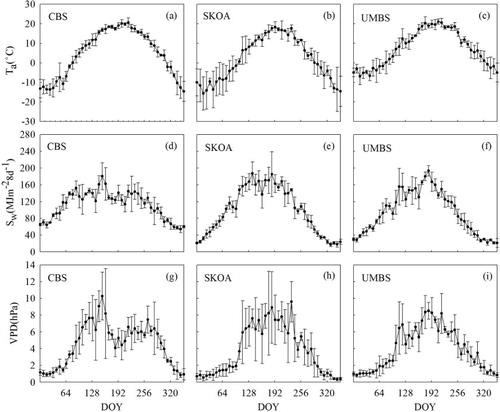
Fig. 2 Monthly cumulative precipitation, PPT: at (a) CBS, (b) SKOA and (c) UMBS.

3.2. Seasonal changes in VIs

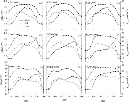
Figure 3 (a–i) shows the seasonal changes in NDVI and EVI from MODIS. At CBS, over all 3 yr, NDVI increased from Day of Year (DOY) 121 to the maximum on DOY 169, kept relatively steady during DOY 169–241, and then decreased. At SKOA, NDVI showed similar seasonal changes to that at CBS, that is, a rapid increase in spring to a maximum in early summer, remaining steady from DOY 169–241, and finally decreasing. At UMBS, similar seasonal changes occurred, but the steady condition lasted longer (DOY 161–257) than that at CBS and SKOA. Overall, NDVI time series at the three sites were distinguishable by prolonged constant high values and asymmetric patterns.

At CBS, EVI exhibited similar seasonal changes in all 3 yr, increasing from early spring (DOY 121) to a maximum in mid-summer (DOY 185) and decreasing thereafter. During the period of increase (DOY 121–185), EVI was the highest in 2004 and lowest in 2005. During the period of decrease (DOY 185–289), EVI was the highest in 2005 and lowest in 2003. At SKOA, EVI increased rapidly at first, reaching the highest on DOY 193 in 2000, and DOY 185 in 2001 and 2002. During the period of increase (DOY 121–185/193), EVI was the highest in 2001 and the lowest in 2002. During the period of decrease (DOY 193–289), there were almost no differences among the EVI trends in the 3 yr. At UMBS, EVI increased at first, reached a maximum in June (during DOY 169–185) of each year, and then decreased slowly. During the period of increase, EVI in 2000 and 2001 was higher than in 2002, and during the decreasing phase, EVI values in 2000 and 2001 were lower than in 2002. Overall, in comparison to NDVI, EVI had no prolonged periods with constant high values at the three sites, and the timing of each seasonal EVI peak was different, as was the EVI behaviour in the summer.

3.3. Inter-annual and seasonal variations of V_cmax

In the EnKF data assimilation process, the parameters were updated daily. Since there were some fluctuations in the optimised parameters at daily time steps, the seasonal variation in the parameter values was represented with their 8 d averages to coincide with the MODIS spectral vegetation indices. The growing season at CBS, SKOA and UMBS spanned over DOY 120–270 (Guan et al., 2006), DOY 120–270 (Mo et al., 2008) and DOY 130–279 (Gough et al., 2008), respectively. At UMBS, cooler temperatures in 2002 than in 2001 resulted in a considerably delayed (by 20 d) leaf expansion (Gough et al., 2008). Therefore, V_cmax during DOY 121–289 was considered as the growing season V_cmax at the three sites in the present study.

Figure 3 (a–i) shows the 8 d averaged V_cmax from DOY 121–289 at the three sites. At CBS, V_cmax showed obvious seasonal variations but almost no inter-annual variation during 2003–2005. It increased slowly from 8.0 µmol m⁻² s⁻¹ with leaf expansion in early spring to a maximum of 32.6 µmol m⁻² s⁻¹ in mid-summer (DOY 217) and then decreased slowly until late autumn (DOY 289). At SKOA, V_cmax showed inter-annual and seasonal variations. In 2000, 2001 and 2002, the peak values of V_cmax were 58.4, 50.5 and 47.3 µmol m⁻² s⁻¹, respectively, which occurred in mid-September (DOY 257). V_cmax in 2002 during DOY 177–257 was much lower than that in 2000 and 2001. This is consistent with the fact that the drought effect in 2002 was more severe than 2001 because stored soil water in 2001 very much minimised any drought effect in that year (Krishnan et al., 2006). At UMBS, V_cmax also showed inter-annual and seasonal variations during 2000–2002. In 2000, V_cmax increased from the early spring (DOY 121) to the beginning of June (DOY 185) and then decreased slightly during June and July (DOY 185–208). Thereafter, it started to increase again at the beginning of August (DOY 217) and approached a second maxima of 35.1 µmol m⁻² s⁻¹ at the end of September (DOY 265) before decreasing to about 8 µmol m⁻² s⁻¹ on DOY 288. In 2001, V_cmax varied similarly to that in 2000, while the second maxima of 30.6 µmol m⁻² s⁻¹ occurred slightly earlier at the beginning of September (DOY 241). In 2002, V_cmax during summer and autumn was much higher than that during the same period of 2000 and 2001 with a maximum value of 39.2 µmol m⁻² s⁻¹ occurring at the beginning of October (DOY 273). However, during spring, it was clearly lower in 2002 than that in 2000 and 2001.

Fig. 3 Seasonal changes in NDVI, EVI and V_cmax: (a–c) for CBS during 2003–2005; (d–f) for SKOA during 2000–2002; and (g–i) for UMBS during 2000–2002.

3.4. Performance of the optimised BEPS model in fluxes simulation

Figure 4 (aa–ci) shows the comparisons of simulated daily GPP, LE and SH with corresponding observations at the three sites. The simulated fluxes presented were the averages of 200 ensemble predictions. With the optimised parameters, BEPS explained, on average, 87–90%, 79% and 79–87% of variations in measured daily LE, SH and GPP, respectively, at CBS, 89–91%, 78–79% and 80–81% at SKOA, and 85–93%, 80–90% and 79–85% at UMBS, respectively. The results indicated that the model closely tracked daily values of measured carbon and energy fluxes in most cases. The statistics for the comparison are presented in Table 3. The slopes and intercepts of regressions between simulated GPP, SH and LE and observations are all close to 1.0 and 0.0, respectively, indicating the excellent ability of the optimised BEPS model to simulate carbon and energy fluxes at these three sites.

Fig. 4 Ensemble daily (24 h) GPP, SH and LE fluxes, and observations: (aa–ai) at CBS during 2003–2005; (ba–bi) at SKOA during 2000–2002; and (ca–ci) at UMBS during 2000–2002. The black and grey dots showed predicted and observed GPP, SH and LE, respectively.

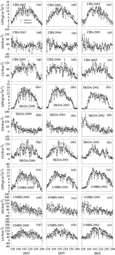
Table 3. Statistics of the linear regression (Y=aX+b) between observed (as Y) and simulated (as X) daily fluxes of GPP (g C m⁻² d⁻¹), LE (W m⁻²) and SH (W m⁻²)

			Parameters optimised using EnKF
Site	ITEM	Year	a	b	R^2	RMSE
CBS	GPP	2003	0.85	1.00	0.89	3.09
		2004	0.89	0.92	0.90	2.99
		2005	0.87	1.14	0.87	2.99
	SH	2003	1.11	−2.61	0.79	25.13
		2004	1.01	−1.49	0.79	24.46
		2005	0.89	4.64	0.79	24.60
	LE	2003	0.91	5.99	0.87	28.92
		2004	0.92	7.63	0.80	26.15
		2005	0.89	7.99	0.79	24.68
SKOA	GPP	2000	0.80	0.56	0.91	4.08
		2001	0.82	1.00	0.91	4.03
		2002	0.92	0.46	0.89	3.52
	SH	2000	0.81	2.28	0.78	37.14
		2001	0.92	−1.76	0.78	28.92
		2002	0.89	−3.19	0.79	47.43
	LE	2000	0.93	3.92	0.81	36.41
		2001	1.04	4.21	0.80	37.65
		2002	1.01	3.25	0.81	29.09
UMBS	GPP	2000	0.86	1.24	0.86	3.11
		2001	0.82	0.62	0.85	3.10
		2002	0.85	0.11	0.93	3.95
	SH	2000	1.05	−18.96	0.90	45.24
		2001	0.85	−10.54	0.80	35.81
		2002	0.93	−9.29	0.82	40.28
	LE	2000	0.88	−1.09	0.79	33.63
		2001	0.81	−5.54	0.82	35.28
		2002	0.86	−6.44	0.85	43.65

3.5. Relationships between satellite-based NDVI, EVI and optimised V_cmax

As VIs increased from spring to mid-summer, V_cmax also depicted similar behaviour (Fig. 5). However, while VIs kept steady or decreased during July and September, V_cmax continued to increase first and then decreased with decreasing VIs. The maximum VIs mainly occurred during DOY 185–193. The growing season was split into two phenological seasons: first phase of increasing VIs from early spring to mid-summer (DOY 121–193) and second phase of decreasing VIs from mid-summer to early winter (DOY 193–289). There were 22 data pairs for V_cmax and VIs across the whole growing season at each site in every year, including 10 pairs for the first phase and 12 pairs for the second phase.

Fig. 5 Relationships between (aa–ai) NDVI and (ba–bi) EVI and V_cmax over the growing seasons from DOY 121–289 during 2003–2005 at CBS. Data were divided into two phenological phases: first phase (solid circles) and second phase (open circles).

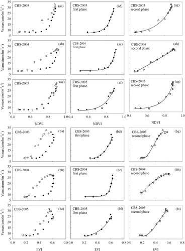
The relationships between V_cmax and VIs (NDVI and EVI) were examined to investigate the predictability of V_cmax from VIs as shown in Fig. 5 for CBS, Fig. 6 for SKOA and Fig. 7 for UMBS. There are four clear patterns in the relationships between V_max and VIs, namely, exponential, and first-, second-, or third-order polynomials. The functions with the highest R² were chosen, and the best regression models between V_cmax and VIs are shown in Table 4.

Fig. 6 Relationships between (aa–ai) NDVI and (ba–bi) EVI and V_cmax over the growing seasons from DOY 121–289 during 2000–2002 at SKOA. Data were divided into two phenological phases: first phase (solid circles) and second phase (open circles).

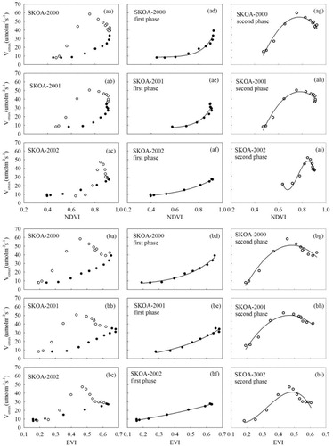
Fig. 7 Relationships between (aa–ai) NDVI and (ba–bi) EVI and V_cmax over the growing seasons from DOY 121–289 during 2000–2002 at UMBS. Data were divided into two phenological phases: first phase (solid circles) and second phase (open circles).

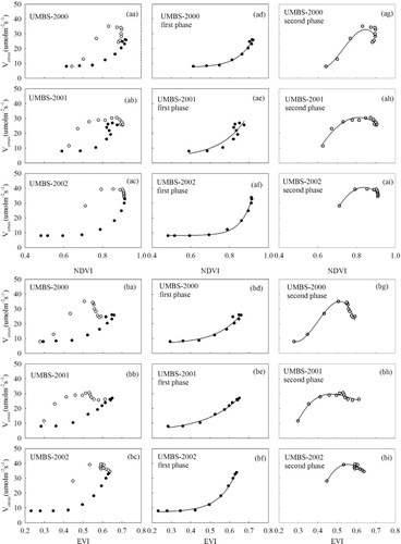
Table 4. Regression results of V_cmax (y, µmol m⁻²s⁻¹) with vegetation indices (NDVI and EVI). Only the best regression models are shown, and the highest R² and significance level are indicated

Site	VIs	Phase	Regression equation	R^2	p
CBS	NDVI	First-2003	y=7.18+3.0781E−005exp(15.23x)	0.99	p<0.001
		Second-2003	y=6.20+0.08exp(6.52x)	0.98	p<0.001
		First-2004	y=8.52+2.5761E−007exp(19.94x)	0.99	p<0.001
		Second-2004	y=−9.57+30.36x+11.37x^2	0.99	p<0.001
		First-2005	y=6.65+0.004exp(9.66x)	0.94	p<0.001
		Second-2005	y=7.40+0.005exp(9.53x)	0.96	p<0.001
	EVI	First-2003	y=5.73+0.14exp(8.10x)	0.95	p<0.001
		Second-2003	y=47.34−438.12x+1468.61x^2−1316.60x^3	0.98	p<0.001
		First-2004	y=8.30+1.0102E−005exp(22.90x)	0.98	p<0.001
		Second-2004	y=13.42−111.80x+530.35x^2−510.84x^3	0.99	p<0.001
		First-2005	y=5.05+0.68exp(5.56x)	0.97	p<0.001
		Second-2005	y=27.55−210.00x+647.11x^2−472.75x^3	0.99	p<0.001
SKOA	NDVI	First-2000	y=8.45+0.002exp(10.25x)	0.95	p<0.001
		Second-2000	y=−277.84+855.21x−552.33x^2	0.96	p<0.001
		First-2001	y=6.52+0.003exp(10.06x)	0.88	p<0.001
		Second-2001	y=−234.28+724.57x−463.69x^2	0.96	p<0.001
		First-2002	y=5.22+0.88exp(3.51x)	0.99	p<0.001
		Second-2002	y=7207.25+7207.25x+38384.699x^2−16744.62x^3	0.96	p<0.001
	EVI	First-2000	y=4.37+1.13exp(5.17x)	0.99	p<0.001
		Second-2000	y=−77.65+530.93x−547.28x^2	0.94	p<0.001
		First-2001	y=−4.86+5.06exp(2.99x)	0.97	p<0.001
		Second-2001	y=−79.73+541.62x−575.89x^2	0.95	p<0.001
		First-2002	y=−16.85+21.22exp(1.17x)	0.99	p<0.001
		Second-2002	y=45.32−531.36x+2127.73x^2+2163.54x^3	0.88	p<0.001
UMBS	NDVI	First-2000	y=7.34+0.0002exp(12.62x)	0.98	p<0.001
		Second-2000	y=1537.02−6582.46x+9256.88x^2−4229.02x^3	0.80	p<0.005
		First-2001	y=3.69+0.03exp(7.73x)	0.80	p<0.001
		Second-2001	y=−306.67+830.96x−511.65x^2	0.93	p<0.001
		First-2002	y=8.141+5.2163E−006exp(16.80x)	0.99	p<0.001
		Second-2002	y=−505.51+1303.61x−777.90x^2	0.89	p<0.001
	EVI	First-2000	y=6.39+0.09exp(8.19x)	0.95	p<0.001
		Second-2000	y=251.32−2086.41x+5672.25x^2−4730.79x^3	0.97	p<0.001
		First-2001	y=4.26+0.57exp(5.71x)	0.99	p<0.001
		Second-2001	y=−190.30+1223.58x−2216.50x^2+1296.40x^3	0.96	p<0.001
		First-2002	y=7.16+0.02exp(11.48x)	0.99	p<0.001
		Second-2002	y=−492.03+2341.052x−3581.89x^2+1669.97x^3	0.90	p<0.001

Figure 5 shows the relationships of V_cmax with NDVI (Fig. 5aa–ai) and EVI (Fig. 5ba–bi) at CBS. Both in the first and second phases, V_cmax showed significant relationships with NDVI (p<0.001, R²=0.94–0.99) and EVI (p<0.001, R²=0.95–0.99) during 2003–2005 (Table 4). In 2003 and 2005, the relationships between V_cmax and NDVI were exponential in both the first and second phases, but in 2004, the relationship was exponential in the first phase and polynomial in the second phase. V_cmax varied exponentially with EVI in the first phase and polynomially in the second phase during the 3 yr.

Figure 6 demonstrates the relationships between V_cmax and NDVI (Fig. 6aa–ai) and EVI (Fig. 6ba–bi) at SKOA. Both in the first and second phases during 2000–2003, V_cmax was significantly correlated with NDVI (p<0.001, R²=0.88–0.99) and EVI (p<0.001, R²=0.88–0.99) (Table 4). V_cmax varied exponentially with VIs (NDVI and EVI) in the first phase, and polynomially in the second phase in all 3 yr.

Figure 7 shows the relationships of V_cmax with NDVI (Fig. 7aa–ai) and EVI (Fig. 7ba–bi) at UMBS. V_cmax was significantly correlated with NDVI and EVI, especially in the first phase (Table 4). EVI performed better than NDVI in predicting V_cmax. Similar to that at SKOA, V_cmax varied exponentially with VIs (NDVI and EVI) in the first phase, and polynomially in the second phase at UMBS.

4. Discussion

4.1. The seasonal hysteresis of V_cmax to NDVI and EVI

The relationships between V_cmax and VIs have been studied earlier by Wang et al. (2008a, 2009) and Jin et al. (2012). However, coefficient of determination was relatively low (most R²<0.8) because they ignored the hysteresis of V_cmax in relation to VIs. In our study, the seasonal hysteresis of V_cmax in relation to NDVI and EVI was apparent at the three sites, as V_cmax increased relatively slowly from spring to mid-summer with increasing VIs and continued increasing even with the VIs keeping steady or deceasing during July and September. Accordingly, the relationships between V_cmax and VIs improved greatly (most R²>0.95) when the growing period was divided into two phases. The hysteresis of V_cmax in relation to VIs could be mainly due to a hysteresis between the leaf chlorophyll content and VIs. It was well known that chlorophyll is one of the more important foliar biochemicals related to the presence of photosynthetic biomass, which is conceptually related to GPP (Sellers et al., 1992) and V_cmax. Also, Dash and Curran (2004) indicated that there was an asymptotic relationship between NDVI and leaf chlorophyll content, Harris and Dash (2010) found that there was a time lag between EVI and GPP, and Shen et al. (2014) also found that EVI failed to closely capture the seasonal changes in canopy photosynthesis in many ecosystems. The time lag or an asymptote between VIs and V_cmax probably results in different variations patterns of V_cmax with VIs during the increasing and decreasing VIs, respectively.

4.2. The potential of satellite-based VIs for V_cmax estimation

Previous studies mainly established the relationships between V_cmax and ground-based broadband and hyperspectral narrow band VIs at the site scale. In the study of Jin et al. (2012), satellite-based VIs (MODIS VIs) were used as indicators for V_cmax, but noise in MODIS VIs was adjusted with ground-based narrow band VIs so that the combination of ground-based narrow band VIs and MODIS VIs could be used to estimate V_cmax. However, it was still not clear if the satellite-based VIs without ground-based VIs as supplements could be used to estimate V_cmax. In this study, the close relationship between V_cmax and MODIS VIs was identified when considering the hysteresis of V_cmax to VIs. This indicates that MODIS VIs can be used for estimating V_cmax at regional or global scales, at least for mixed and broadleaf forests. Furthermore, the well-known saturation effect of NDVI would have caused it to stay at constant high values despite decreases in canopy greenness. The timing of the slightly different seasonal maxima of NDVI and EVI and also different behaviours of VIs in summer period (relatively stable NDVI but a steep decrease in EVI) would have influenced relationships between V_cmax and VIs (NDVI and EVI).

4.3. Accounting for seasonal V_cmax behaviour

Modelled V_cmax showed temporal variations at the three sites, which was consistent with findings of previous studies involving field measurement and model inversion (e.g., Kosugi and Matsuo, 2006; Misson et al., 2006; Zhang, 2006; Wang et al., 2007, 2008b; Mo et al., 2008; Muraoka et al., 2012). Our results that V_cmax could be affected by drought confirmed earlier findings (Wang et al., 2007; Keenan et al. 2009; Ju et al., 2010). At SKOA, the lower V_cmax values during the leaf expansion stage in 2001 and 2002 were related to drought in these 2 yr. At UMBS, during June and July (DOY 185–208) of 2000 and 2001, there were decreases in V_cmax, which were probably due to high temperatures and relatively low soil water availability caused by low precipitation amounts of 7.7 mm in 2000 and 33.8 mm in 2001, compared with 43.8 mm in 2002. Moreover, V_cmax may also be affected by cool temperature (Gough et al., 2008). In 2002, during the increasing phase, V_cmax was continuously lower than during the same period in 2000 and 2001, while during the decreasing phase, the higher values lasted longer in 2002 than during 2000 and 2001. Cooler temperatures in 2002 than in 2001 resulted in a considerably delayed (by 20 d) leaf expansion in 2002.

The spatial representativeness of many flux measurements at forest ecosystems is several hundred meters to several kilometres, for example, about 1000–3000 m for ChinaFlux forest ecosystems (Mi et al., 2006). The spatial resolution of flux measurements at forest ecosystems is probably of the same order of magnitude as the satellite data. Therefore, compared with direct gas-exchange measurements of V_cmax at leaf scale, seasonal parameter values optimised using EC measurement at ecosystem scale would be more suitable for estimating V_cmax at regional scales by combining with satellite data. However, for estimating spatial and temporal distributions of V_cmax using satellite-based VIs, we need to generalise these relationships, for example, one relationship each for increasing and decreasing phases for a given site and then extending these to other sites with different plant types. This will help in estimating temporal variation in V_cmax at regional or global scales, thereby contributing to more precise carbon cycle modelling.

5. Conclusions

The EnKF data assimilation is an effective technique for model parameter optimisation. Optimised V_cmax showed considerable seasonal and inter-annual variations in mixed and deciduous forest ecosystems. V_cmax increased with leaf expansion in early spring to a maximum in mid-summer and then decreased slowly until early winter.

Seasonal hysteresis of V_cmax in relation to NDVI and EVI was found for mixed and deciduous forest ecosystems. When the growing period was divided into two periods, namely, increasing V_cmax and decreasing V_cmax stages, the relationships between V_cmax and VIs were greatly improved. In the first phase (May to mid-July), V_cmax varied with NDVI and EVI exponentially but polynomially in the second phase (mid-July to mid-October).

The relationships between V_cmax and NDVI and EVI improved when seasonal hysteresis of V_cmax in relation to NDVI and EVI was considered. Both satellite-based NDVI and EVI could be used to better predict V_cmax of deciduous and mixed forests by dividing the growing period into increasing and decreasing V_cmax periods. These results would be helpful for estimating spatial and temporal distributions of V_cmax using satellite-based VIs in the future. However, it should be kept in mind that there are still some uncertainties, such as unrealistic fluctuations of NDVI and EVI caused by residual cloud contamination, and the utility of atmospheric noise removal using the LACC method.

6. Acknowledgements

This research was supported by National Basic Research Program of China (2010CB950702) and National Natural Science Foundation of China (41371070). The authors greatly thank researchers of Changbai Mountain experiment station, Saskatchewan BERMS Old Aspen site and University of Michigan Biological Station for providing fluxes and meteorological data, and Professor Scott Munro, University of Toronto, for editing this manuscript.

References

- Aalto T. , Ciais P. , Chevillard A. , Moulin C . Optimal determination of the parameters controlling biospheric CO2 fluxes over Europe using eddy covariance fluxes and satellite NDVI measurements. Tellus B. 2004; 56: 93–104.
- Ball J. T. , Woodrow I. E. , Berry J. A . Biggins J . A model predicting stomatal conductance and its contribution to the control of photosynthesis under different environmental conditions. Progress in Photosynthetic Research. 1987; Dordrecht: Martinus Nijhoff Publishers. 221–224.
- Bonan G. B . Land atmosphere CO2 exchange simulated by a land-surface process model coupled to an atmospheric general-circulation model. J. Geophys. Res. Atmos. 1995; 100: 2817–2831.
- Carter G. A . Reflectance wavebands and indices for remote estimation of photosynthesis and stomatal conductance in pine canopies. Rem. Sens. Environ. 1998; 63: 61–72.
- Chen J. M. , Deng F. , Chen M . Locally adjusted cubic-spline capping for reconstructing seasonal trajectories of a satellite-derived surface parameter. IEEE Trans. Geosci. Rem. Sens. 2006; 44: 2230–2238.
- Chen J. M. , Liu J. , Cihlar J. , Goulden M. L . Daily canopy photosynthesis model through temporal and spatial scaling for remote sensing applications. Ecol. Model. 1999; 124: 99–119.
- Chen J. M. , Mo G. , Pisek J. , Liu J. , Deng F. , co-authors . Effects of foliage clumping on global terrestrial gross primary productivity. Global Biogeochem. Cy. 2012; 26: 1019.
- Choudhury B. J . Estimating gross photosynthesis using satellite and ancillary data: approach and preliminary results. Rem. Sens. Environ. 2001; 75: 1–21.
- Curtis P. S. , Vogel C. S. , Gough C. M. , Schmid H. P. , Su H. B. , co-authors . Respiratory carbon losses and the carbon-use efficiency of a northern hardwood forest, 1999–2003. New Phytol. 2005; 167: 437–455.
- Dash J. , Curran P. J . The MERIS terrestrial chlorophyll index. Int. J. Rem. Sens. 2004; 25(23): 5403–5413.
- Desai A. R. , Richardson A. D. , Moffat A. M. , Kattge J. , Hollinger D. Y. , co-authors . Cross-site evaluation of eddy covariance GPP and RE decomposition techniques. Agr. Forest Meteorol. 2008; 148: 821–838.
- Dobrowski S. Z. , Pushnik J. C. , Zarco-Tejada P. J. , Ustin S. L . Simple reflectance indices track heat and water stress-induced changes in steady-state chlorophyll fluorescence at the canopy scale. Rem. Sens. Environ. 2005; 97: 403–414.
- Elbers J. A. , Jacobs C. M. J. , Kruijt B. , Jans W. W. P. , Moors E. J . Assessing the uncertainty of estimated annual totals of net ecosystem productivity: a practical approach applied to a mid latitude temperate pine forest. Agr. Forest Meteorol. 2011; 151: 1823–1830.
- Falge E. , Baldocchi D. , Olson R. , Anthoni P. , Aubinet M. , co-authors . Gap filling strategies for long term energy flux data sets. Agr. Forest Meteorol. 2001a; 107: 71–77.
- Falge E. , Baldocchi D. , Olson R. , Anthoni P. , Aubinet M. , co-authors . Gap filling strategies for defensible annual sums of net ecosystem exchange. Agr. Forest Meteorol. 2001b; 107: 43–69.
- Fan Y. Z. , Zhong Z. M. , Zhang X. Z . Determination of photosynthetic parameters Vcmax and Jmax for a C3 plant (spring hulless barley) at two altitudes on the Tibetan Plateau. Agr. Forest Meteorol. 2011; 151(12): 1481–1487.
- Farquhar G. D. , Caemmerer S. V. , Berry J. A . A biochemical-model of photosynthetic CO2 assimilation in leaves of C3 species. Planta. 1980; 149: 78–90.
- Field C. B. , Randerson J. T. , Malmstrom C. M . Global net primary production-combining ecology and remote-sensing. Rem. Sens. Environ. 1995; 51: 74–88.
- Gamon J. A. , Field C. B. , Goulden M. L. , Griffin K. L. , Hartley A. E. , co-authors . Relationships between NDVI, canopy structure, and photosynthesis in 3 Californian vegetation types. Ecol. Appl. 1995; 5: 28–41.
- Gamon J. A. , Surfus J. S . Assessing leaf pigment content and activity with a reflectometer. New Phytol. 1999; 143: 105–117.
- Gitelson A. A. , Gurlin D. , Moses W. J. , Barrow T . A bio-optical algorithm for the remote estimation of the chlorophyll-a concentration in case 2 waters. Environ. Res. Lett. 2009; 4: 045003.
- Gough C. M. , Hardiman B. S. , Nave L. E. , Bohrer G. , Maurer K. D. , co-authors . Sustained carbon uptake and storage following moderate disturbance in a Great Lakes forest. Ecol. Appl. 2013; 23: 1202–1215.
- Gough C. M. , Vogel C. S. , Schmid H. P. , Su H. B. , Curtis P. S . Multi-year convergence of biometric and meteorological estimates of forest carbon storage. Agr. Forest Meteorol. 2008; 148: 158–170.
- Goulden M. L. , Munger J. W. , Fan S. M. , Daube B. C. , Wofsy S. C . Measurements of carbon sequestration by long-term eddy covariance: methods and a critical evaluation of accuracy. Global Change Biol. 1996; 2: 169–182.
- Gower S. T. , Vogel J. G. , Norman J. M. , Kucharik C. J. , Steele S. J. , co-authors . Carbon distribution and aboveground net primary production in aspen, jack pine, and black spruce stands in Saskatchewan and Manitoba, Canada. J. Geophys. Res. Atmos. 1997; 102: 29029–29041.
- Grant R. F. , Zhang Y. , Yuan F. , Wang S. , Hanson P. J. , co-authors . Intercomparison of techniques to model water stress effects on CO2 and energy exchange in temperate and boreal deciduous forests. Ecol. Model. 2006; 196(3–4): 289–312.
- Grassi G. , Vicinelli E. , Ponti F. , Cantoni L. , Magnani F . Seasonal and interannual variability of photosynthetic capacity in relation to leaf nitrogen in a deciduous forest plantation in northern Italy. Tree Physiol. 2005; 25: 349–360.
- Guan D. X. , Wu J. B. , Zhao X. S. , Han S. J. , Yu G. R. , co-authors . CO2 fluxes over an old, temperate mixed forest in northeastern China. Agr. Forest Meteorol. 2006; 137: 138–149.
- Harris A. , Dash J . The potential of the MERIS Terrestrial Chlorophyll Index for carbon flux estimation. Rem. Sens. Environ. 2010; 114: 1856–1862.
- Hoffmann F . FAGUS, A model for growth and development of beech. Ecol. Model. 1995; 83: 327–348.
- Horn J. E. , Schulz K . Identification of a general light use efficiency model for gross primary production. Biogeosciences. 2011; 8: 999–1021.
- Houborg R. , Cescatti A. , Migliavacca M. , Kustas W. P . Satellite retrievals of leaf chlorophyll and photosynthetic capacity for improved modeling of GPP. Agr. Forest Meteorol. 2013; 177: 10–23.
- Jin P. , Wang Q. , Iio A. , Tenhunen J . Retrieval of seasonal variation in photosynthetic capacity from multi-source vegetation indices. Ecol. Informat. 2012; 7: 7–18.
- Ju W. , Chen J. M. , Black T. A. , Barr A. G. , Liu J. , co-authors . Modelling multi-year coupled carbon and water fluxes in a boreal aspen forest. Agr. Forest Meteorol. 2006; 140: 136–151.
- Ju W. , Wang S. , Yu G. , Zhou Y. , Wang H . Modeling the impact of drought on canopy carbon and water fluxes for a subtropical evergreen coniferous plantation in southern China through parameter optimization using an ensemble Kalman filter. Biogeosciences. 2010; 7: 845–857.
- Keenan T. , Garcia R. , Friend A. D. , Zaehle S. , Gracia C. , co-authors . Improved understanding of drought controls on seasonal variation in Mediterranean forest canopy CO2 and water fluxes through combined in situ measurements and ecosystem modelling. Biogeosciences. 2009; 6: 1423–1444.
- Kimball J. S. , Keyser A. R. , Running S. W. , Saatchi S. S . Regional assessment of boreal forest productivity using an ecological process model and remote sensing parameter maps. Tree Physiol. 2000; 20: 761–775.
- Kosugi Y. , Shibata S. , Kobashi S . Parameterization of the CO2 and H2O gas exchange of several temperate deciduous broadleaved trees at the leaf scale considering seasonal changes. Plant Cell Environ. 2003; 26: 285–301.
- Kosugi Y. , Matsuo N . Seasonal fluctuations and temperature dependence of leaf gas exchange parameters of co-occurring evergreen and deciduous trees in a temperate broad-leaved forest. Tree Physiol. 2006; 26: 1173–1184.
- Krishnan P. , Black T. A. , Grant N. J. , Barr A. G. , Hogg E. H. , co-authors . Impact of changing soil moisture distribution on net ecosystem productivity of a boreal aspen forest during and following drought. Agr. Forest Meteorol. 2006; 139: 208–223.
- Lasslop G. , Reichstein M. , Kattge J. , Papale D . Influences of observation errors in eddy flux data on inverse model parameter estimation. Biogeosciences. 2008; 5: 1311–1324.
- Lloyd J. , Taylor J. A . On the temperature-dependence of soil respiration. Funct. Ecol. 1994; 8: 315–323.
- Lu X. , Kicklighter D. W. , Melillo J. M. , Yang P. , Rosenzweig B. , co-authors . A contemporary carbon balance for the Northeast region of the United States. Environ. Sci. Tech. 2013; 47(23): 13230–13238.
- Mi N. , Yu G. R. , Wang P. X. , Wen X. F. , Sun X. M . A preliminary study for spatial representiveness of flux observation at ChinaFLUX sites. Sci. China Earth. Sci. 2006; 49: 24–35.
- Misson L. , Tu K. P. , Boniello R. A. , Goldstein A. H . Seasonality of photosynthetic parameters in a multi-specific and vertically complex forest ecosystem in the Sierra Nevada of California. Tree Physiol. 2006; 26: 729–741.
- Mo X. , Chen J. M. , Ju W. , Black T. A . Optimization of ecosystem model parameters through assimilating eddy covariance flux data with an ensemble Kalman filter. Ecol. Model. 2008; 217: 157–173.
- Moradkhani H. , Sorooshian S. , Gupta H. V. , Houser P. R . Dual state-parameter estimation of hydrological models using ensemble Kalman filter. Adv. Water Resour. 2005; 28: 135–147.
- Muraoka H. , Noda H. M. , Nagai S. , Motohka T. , Saitoh T. M. , co-authors . Spectral vegetation indices as the indicator of canopy photosynthetic productivity in a deciduous broadleaf forest. J. Plant Ecol. 2012; 6: 393–407.
- Reichstein M. , Tenhunen J. , Roupsard O. , Ourcival J. M. , Rambal S. , co-authors . Inverse modeling of seasonal drought effects on canopy CO2/H2O exchange in three Mediterranean ecosystems. J. Geophys. Res. Atmos. 2003; 108: D23, 4726.
- Richardson A. D. , Mahecha M. D. , Falge E. , Kattge J. , Moffat A. M. , co-authors . Statistical properties of random CO2 flux measurement uncertainty inferred from model residuals. Agr. Forest Meteorol. 2008; 148: 38–50.
- Running S. W. , Coughlan J. C . A general-model of forest ecosystem processes for regional applications 1. hydrologic balance, canopy gas-exchange and primary production processes. Ecol. Model. 1988; 42: 125–154.
- Santaren D. , Peylin P. , Viovy N. , Ciais P . Optimizing a process-based ecosystem model with eddy-covariance flux measurements: a pine forest in southern France. Global Biogeochem. Cy. 2007; 21: GB2013.
- Schaefer K. , Schwalm C. R. , Williams C. , Arain M. A. , Barr A. , co-authors . A model-data comparison of gross primary productivity: results from the North American Carbon Program site synthesis. J. Geophys. Res. 2012; 117: 03010.
- Sellers P. J. , Berry J. A. , Collatz G. J. , Field C. B. , Hall F. G . Canopy reflectance, photosynthesis, and transpiration. III. A reanalysis using improved leaf models and a new canopy integration scheme. Rem. Sens. Environ. 1992; 42: 187–216.
- Sellers P. J. , Dickinson R. E. , Randall D. A. , Betts A. K. , Hall F. G. , co-authors . Modeling the exchanges of energy, water, and carbon between continents and the atmosphere. Science. 1997; 275: 502–509.
- Shen M. G. , Tang Y. H. , Desai A. R. , Gough C. , Chen J . Can EVI-derived land-surface phenology be used as a surrogate for phenology of canopy photosynthesis?. Int. J. Rem. Sens. 2014; 35(3): 1162–1174.
- Stickan W. , Gansert D. , Neemann G. , Rees U . Modeling the influence of climatic variability on carbon and water budgets of beech saplings (Fagus sylvatica L.) based on field data. Ecol. Model. 1994; 75: 331–343.
- Tu K . Modeling Plant–Soil–Atmosphere CO2 Exchange Using Optimality Principles.
- Vonstamm S . 1994. Linked stomata and photosynthesis model for Corylus avellana (hazel). Ecol. Model. 75, 345–357..
- Wang Q. , Iio A. , Kakubari Y . Broadband simple ratio closely traced seasonal trajectory of canopy photosynthetic capacity. Geophys. Res. Lett. 2008a; 35: L07401.
- Wang Q. , Iio A. , Tenhunen J. , Kakubari Y . Annual and seasonal variations in photosynthetic capacity of Fagus crenata along an elevation gradient in the Naeba Mountains, Japan. Tree Physiol. 2008b; 28: 277–285.
- Wang Q. , Tenhunen J. , Dinh N. Q. , Reichstein M. , Vesala T. , co-authors . Similarities in ground- and satellite-based NDVI time series and their relationship to physiological activity of a Scots pine forest in Finland. Rem. Sens. Environ. 2004a; 93: 225–237.
- Wang Q. , Tenhunen J. , Falge E. , Bernhofer C. , Granier A. , co-authors . Simulation and scaling of temporal variation in gross primary production for coniferous and deciduous temperate forests. Global Change Biol. 2004b; 10: 37–51.
- Wang Q. , Tenhunen J. , Vesala T . Correlated change in normalized difference vegetation index and the seasonal trajectory of photosynthetic capacity in a conifer stand. Int. J. Rem. Sens. 2009; 30: 983–1001.
- Wang Y. P. , Baldocchi D. , Leuning R. , Falge E. , Vesala T . Estimating parameters in a land-surface model by applying nonlinear inversion to eddy covariance flux measurements from eight FLUXNET sites. Global Change Biol. 2007; 13: 652–670.
- Wesely M. , Hart R . Hutchinson B. A. , Hicks B. B . Variability of short term eddy-correlation estimates of mass exchange. The Forest–Atmosphere Interaction. 1985; Springer, New York 591–612.
- Wilson K. B. , Baldocchi D. D. , Hanson P. J . Spatial and seasonal variability of photosynthetic parameters and their relationship to leaf nitrogen in a deciduous forest. Tree Physiol. 2000; 20: 565–578.
- Wilson K. B. , Baldocchi D. D. , Hanson P. J . Leaf age affects the seasonal pattern of photosynthetic capacity and net ecosystem exchange of carbon in a deciduous forest. Plant Cell Environ. 2001; 24: 571–583.
- Xu L. K. , Baldocchi D. D . Seasonal trends in photosynthetic parameters and stomatal conductance of blue oak (Quercus douglasii) under prolonged summer drought and high temperature. Tree Physiol. 2003; 23: 865–877.
- Yu G.-R. , Zhang L.-M. , Sun X.-M. , Fu Y.-L. , Wen X.-F. , co-authors . Environmental controls over carbon exchange of three forest ecosystems in eastern China. Global Change Biol. 2008; 14: 2555–2571.
- Zhang J. , Hu Y. , Xiao X. , Chen P. , Han S. , co-authors . Satellite-based estimation of evapotranspiration of an old-growth temperate mixed forest. Agr. Forest Meteorol. 2009; 149: 976–984.
- Zhang M . Simulation of Photosynthetic Productivity of the Canopy of Broad-Leaved and Korean-Pine Forest in Changbai Mountain. 2006; Beijing: Graduate University of Chinese Academy of Sciences. 44. PhD Thesis.