A feasibility study of mapping light-absorbing carbon using a taxi fleet as a mobile platform

Abstract

Carbon-containing particles are associated with adverse health effects, and their light-absorbing fractions were recently estimated to be the second largest contributor to global warming after carbon dioxide. Knowledge on the spatiotemporal variability of light-absorbing carbon (LAC) particles in urban areas is relevant for air quality management and to better diagnose the population exposure to these particles. This work reports on the first mobile LAC mass concentrations (M_LAC) measured on-board four taxis in the Stockholm metropolitan area in November 2011. On average, concentrations were higher and more variable during daytime (median of 1.9 µg m⁻³ and median absolute deviation of 2.3 µg m⁻³). Night-time (21:00–05:00) measurements were very similar for all road types and also compared to levels monitored at an urban background fixed site (median of 0.9 µg m⁻³). We observed a large intra-urban variability in concentrations, with maxima levels inside road tunnels (median and 95th percentile of 7.5 and 40.1 µg m⁻³, respectively). Highways presented the second ranked concentrations (median and 95th percentile of 3.2 and 9.7 µg m⁻³, respectively) associated with highest vehicle speed (median of 65 km h⁻¹), traffic rates (median of 62 000 vehicles day⁻¹ and 1500 vehicles h⁻¹) and diesel vehicles share (7–10%) when compared to main roads, canyon streets, and local roads. Multiple regression modelling identified hourly traffic rate and M_LAC concentration measured at an urban background site as the best predictors of on-road concentrations, but explained only 25% of the observed variability. This feasibility study proved to be a time- and cost-effective approach to map out ambient M_LAC concentrations in Stockholm and more research is required to represent the distribution in other periods of the year. Simultaneous monitoring of other pollutants, closely correlated to M_LAC levels in traffic-polluted environments, and including video recording of road and traffic changes would be an asset.

• black carbon
• elemental carbon
• mobile measurements
• urban aerosols
• air quality
• multiple regression modelling
• Sweden

To access the supplementary material to this article, please see Supplementary files under Article Tools online.

1. Introduction

Primary carbonaceous aerosols are formed during incomplete combustion of carbon-based fuels, and regarding their optical properties they are classified as light-absorbing carbon (LAC) and organic carbon (OC); the latter has weak absorption in the visible electromagnetic spectrum. Because of their ability to strongly absorb sunlight, LAC affects the Earth's climate system through various complex mechanisms contributing to global warming. Bond et al. (2013) recently estimated that LAC particles are the second most important man-made agent of climate change, right after carbon dioxide. On a planetary scale, and assuming a perpetual constant 2000 emissions, the largest LAC-related radiative forcing per economic sector for the year 2020 corresponds to biomass burning, household biofuel and on-road transportation (Unger et al., 2010). In Sweden, the main sources of LAC emissions in 2005 were residential combustion of biofuels (37%), road transport (21%), off-road transport (18%) and power plants/industry (18%) (Hansson et al., 2011).

Besides the relevant climate impacts, carbon-containing aerosols are associated with cardiopulmonary morbidity and mortality since they act as carriers of a wide variety of toxic chemical constituents (Janssen et al., 2012). LAC particles make up a large fraction of diesel transport emissions (on average, ~75%) and, lately, the World Health Organization reclassified diesel exhaust fumes from ‘probably carcinogenic’ to ‘carcinogenic’ due to compelling scientific evidence (Attfield et al., 2012; Silverman et al., 2012). Thus, the implementation of strategies to reduce LAC emissions should be of outmost importance to decrease people's exposure to them, as well as providing almost immediate climate benefits.

A detailed knowledge of the concentration variability across the city is required to better predict the daily exposure of the general population and of drivers, identify air quality hot-spot areas, and elucidate the factors determining pollutant emissions. Spatiotemporal characteristics of ambient aerosol are commonly investigated by simultaneous measurements at fixed sites, by remote sensing (aircrafts and satellites) and, less frequently, by using ground-based mobile platforms. Mobile platforms provide a larger spatial coverage than a network of stationary monitoring sites and can be used either for stationary sampling (i.e. parked for on-going monitoring) or for drive-by measurements (i.e. measuring while driving). Mobile air quality laboratories usually have a large set of gas and aerosol rapid-response instruments deployed on permanently dedicated vehicles (passenger cars, vans, trucks and even trains) and follow a selected route within the city on a regular basis for a relatively brief time (usually a few hours). Some experiments are designed to chase single vehicle emissions such as diesel engine exhaust plumes to construct or verify emission inventories (e.g. Wang et al., 2011). Other researchers focus on mapping the concentration distribution of atmospheric pollutants (e.g. Mohr et al., 2011) whereas some studies target specific city areas such as traffic-dominated regions (e.g. Pirjola et al., 2004) and industrial neighbourhoods (Wallace et al., 2009). Mobile monitoring studies, including M_LAC measurements, were performed in several cities like Zurich in Switzerland (Mohr et al., 2011), Aachen in Germany (Schneider et al., 2008), Beijing in China (Wang et al., 2009), Mexico City in Mexico (Thornhill et al., 2008) and Los Angeles in USA (Westerdahl et al., 2005).

Stockholm is the most populous metropolitan region in Scandinavia (2.1 million inhabitants, Statistics Sweden, 2012) and is built over 14 islands with over 30% of the area made up of waterways and 30% occupied by green spaces. To interconnect the islands and speed up road transport, several bridges and road tunnels are in use and two large road projects consisting of long tunnels (Norra Länken and E4 Stockholm Bypass) are under construction. To comply with national and EU air quality directives, an air quality monitoring network was established in Stockholm in 1993–1994 by the Stockholm Environment and Health Administration and is operated by SLB analys. A previous study by Krecl et al. (2011) analysed measurements carried out at four monitoring stations (two kerbside stations, one urban background site and a rural station) in Stockholm to determine the spatial variability of LAC mass concentrations (M_LAC) within the city. They concluded that concentrations of LAC between urban sites were poorly correlated (even for daily averages) and highly heterogeneously distributed. This finding emphasises the need for a more detailed mapping of pollutants levels in the city to better assess the population exposure.

This work examines the first mobile LAC measurements conducted in the Stockholm metropolitan area during an intensive campaign in November 2011. Unlike other studies, we installed instruments on-board taxis operating on their usual working schedule, with no planned route. We aim to show that this novel approach is suitable for mapping out the intra-urban M_LAC concentrations with high spatiotemporal resolution. After characterising the mobile concentrations, we combined them with fixed-site monitoring and traffic factors into a multiple regression model to identify the best predictors of on-road LAC.

2. Methodology

Concurrent mobile and fixed M_LAC concentrations were collected in the Stockholm metropolitan area during 7–17 November 2011, along with geolocation and vehicle speed (mobile), and meteorological variables (stationary sites). A description of the experimental set-up and the strategy for data analysis follows.

2.1. Mobile measurements

On-road measurements were performed simultaneously by using four diesel taxis as mobile platforms. Concentrations of M_LAC were gathered with Micro Aethalometers model AE51 (Magee Scientific, USA) at 880 nm wavelength, with no pre-cut size device and the LAC mass absorption cross section σ_a provided by the manufacturer (12.5 m² g⁻¹) was used to compute Aethalometer concentrations. Flow rates were setup initially at 100 ml min⁻¹, but after gaining experience on the typical filter loading with these sampling conditions, the flow rates were lowered to 40–50 ml min⁻¹. Vehicle geographical position and driving speed were recorded with portable global positioning system (GPS) data loggers (GlobalSat model DG-100, Taiwan). The instruments were housed in a small box (23×14×10 cm) on the taxi rooftop towards the left centre location using the taxi roof-light structure to mount the box, approximately 1.5 m above the road surface. This position was chosen to reduce, as much as possible, self-contamination by the engine exhaust emissions. The GPS logged data every 6 sec., and the micro Aethalometer recorded M_LAC measurements every minute. Always when batteries were changed, the clocks of the instruments were synchronised according to the satellite time given by the GPS. Mobile M_LAC data were screened for high attenuation values (ATN>75, Virkkula et al., 2007), low battery charge, flow rate out of range, and LED current out of range. Measurements matching periods of maintenance and when taxis were parked at the company garage were also excluded. GPS data were examined to detect wrong geolocations and causes of temporary signal interruption (inside road tunnels or low battery events).

2.2. Fixed-site monitoring

Stationary M_LAC measurements were carried out at two monitoring sites in central Stockholm (Hornsgatan and Torkel) and at a rural station (Aspvreten) using custom-built Particle Soot Absorption Photometers (PSAPs) with no size selective inlet at a 525 nm wavelength (Krecl et al., 2010, 2011). Data were logged every 15 min and several corrections were applied to PSAP measurements to obtain the absorption coefficient of the airborne particles (Krecl et al., 2007, 2010, 2011). To correct for light scattered from aerosol deposited onto the PSAP filter, aerosol light-scattering coefficients were estimated from PM_2.5 mass concentrations multiplied by aerosol mass scattering coefficients of 4.0 and 2.0 m² g⁻¹ for urban and rural sites, respectively (Krecl et al., 2007, 2011). Finally, to convert the aerosol light absorption coefficient into M_LAC we used site-dependent σ_a values of 7.6 and 10 m² g⁻¹ for urban and rural sites, respectively (Krecl et al., 2011). We assumed that all light absorption was from LAC and that all LAC had the same σ_a value at each site over the sampling period. We discarded the contribution of other light-absorbing substances (e.g. mineral dust) to the PSAP measurements since no dust re-suspension occurs in Stockholm during the fall season (Norman and Johansson, 2006) and no long-range transport of Saharan mineral dust to Stockholm was observed during the sampling period (4-d air mass backward trajectory analysis with HYSPLIT, Draxler and Rolph, 2013).

Hornsgatan is a four-lane street canyon and instruments were housed in a trailer parked on the street with a traffic volume of ~28 000 vehicles per day. Torkel is located on a rooftop platform (25 m height) and thereby represents urban background concentrations for the Stockholm region, since it is less affected by nearby emissions. The distance between Hornsgatan and Torkel sites is 450 m. Aspvreten is a rural background station, operated by ITM (Stockholm University), and located 80 km southwest of Stockholm in a region with forest and grasslands.

In addition, meteorological measurements were conducted at Torkel site, including air temperature and relative humidity (Hygroclip probe, Rotronic AG, Switzerland), precipitation (tipping bucket rain gauge, model HB 3166-06, Casella Measurement, UK), and wind speed and direction (ultrasonic anemometer, model R3, Gill Instruments Ltd., UK). Sensors were installed at 2 m above rooftop, except for the anemometer installed at 10 m height, and hourly averages were recorded. All data are reported in local standard time (UTC+1).

2.3. Traffic and population information

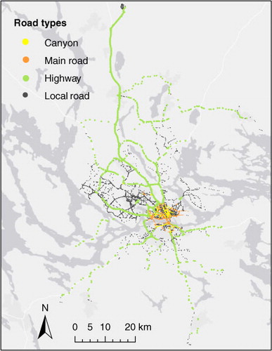
Population density is often used as a proxy for anthropogenic activities, including vehicular traffic, whereas more specific traffic variables better describe the impact of on-road traffic. We used population density for the Stockholm and Uppsala counties, expressed in number of inhabitants per km², provided by Statistics Sweden. The following data fields from the Swedish National Road database (Norlin, 2013): geocoded location, daily traffic counts, heavy-duty share, road type and road speed limit were used to assess the traffic rate and road characteristics for each individual waypoint in our study. Daily traffic rates, based on annual average counts including light- and heavy-duty vehicles travelling in both directions, were informed by the Stockholm and Uppsala County Air Quality Management Association (LVF) for the region of interest. In theory, the road network includes all roads for motorised vehicles, and the requirement of positional accuracy for road links is ±4 m at the 95% confidence level (Norlin, 2013). For this study, road types were grouped into the following categories: highways, main roads, canyon streets, local roads and tunnel roads (Fig. 1). Note that geographical positions of road tunnels were not mapped due to their small dimensions in relation to the map scale. Street canyons are mostly located on main roads (81%), but were classified in a separate group because of their special geometry, which prevents pollutants from a proper dispersion when wind blows perpendicular to the canyon orientation (Vardoulakis et al., 2003). Diurnal profiles of traffic rate for the different road types, months and days of the week (Monday–Thursday, Friday, Saturday and Sunday) were extracted from the LVF emission database (Johansson and Eneroth, 2007) and later used to calculate traffic rates for light-duty vehicles for each waypoint of our dataset.

Fig. 1 Map of the roads sampled in the Stockholm metropolitan region.

2.4. Data processing and integration

To highlight spatial variations in the concentrations, a temporal adjustment of mobile M_LAC concentrations was performed following a combined approach as suggested by Dons et al. (2012). Then, hourly mean observations from a reference monitor (Aspvreten rural site) were used to rescale the mobile measurements. Depending on the relationship between the mobile and background concentrations at a particular day and time, an additive or multiplicative term was used to temporally adjust the on-road M_LAC concentration and account for changing background conditions (for details on the methodology, see Supplementary file).

Median GPS variables (i.e. latitude, longitude and vehicle speed) were calculated over 1-min periods matching the sampling times of valid mobile concentrations. We discarded measurements with missing GPS signal due to low battery charge, whereas data with no associated GPS signal inside road tunnels were preserved for further analysis. Using geospatial processing software (ArcGis 10, ESRI, Redlands, USA), the geocoded 1-min M_LAC observations were linked to the road and traffic data associated with the road network previously described. The spatial joint was done using the nearest road link and different arbitrary cut-off distances were considered for data exclusion: 400, 100 and 30 m. A threshold of 100 m was decided based on a trade-off between data accuracy and data reduction (see detailed explanation in Supplementary file). Finally, the geocoded M_LAC dataset with traffic attributes was spatially joined with the population density layer.

2.5. Statistical analysis

Descriptive statistics and temporal variations were calculated for mobile and fixed-site M_LAC concentrations, and bivariate relationships between mobile M_LAC concentration and traffic-related variables were explored.

Afterwards stepwise multiple regression was performed to examine the relationship between a single dependent variable (mobile M_LAC data) and a set of independent variables (numerical and categorical), and to predict on-road M_LAC concentrations as a function of several predictors. Prior to model fitting, independent variables were selected to reduce multicollinearity following Henderson et al. (2007). First, we analysed the Pearson correlation coefficient (r) matrix of the numerical independent variables. If two independent variables were highly correlated (∣r∣>0.95), the one with the lowest correlation with the dependent variable was deleted. Second, we identified the independent variable with the highest correlation with the dependent variable in each subcategory. Variables in the same subcategory that were moderately correlated (∣r∣>0.6) with the most highly ranked variable were also discarded. Categorical variables were included in the model through indicator coding with the condition that each subcategory should at least contain 10% of the observations (Noth et al., 2011). The pool of candidate variables was also checked for normality (normal probability plots), linearity and homoscedasticity (bivariate plots) and remedy transformations were applied, when possible, for assumption violations.

The regression process started with a constant model and used a linear model as the upper bounding model. The criterion used for inclusion of independent variables at any step was their contribution to the adjusted coefficient of determination (adjusted R²), set up to at least 1%. Variables with insignificant t-statistics at a confidence level of 95% were removed. A second model run included a non-linear effect to allow interactions within the independent variables in the form of a bilinear moderator. To further determine assumption violations due to the combined effects of all independent variables onto the dependent variable, residual values were examined for normality (normal distribution plots), linearity and homoscedasticity (studentised residuals vs. fitted values), and independence of the error term (Hair et al., 1998). In the latter case, the spatial correlation of studentised residuals was calculated by using the Moran's index and the temporal correlation was explored through autocorrelation analysis. Then, we identified influential observations through a set of diagnostics (leverage, Cook's distance, covariance ratio, and DFFIT) and assessed their impact on the regression model. Besides interpreting the regression variate from the statistical viewpoint, we identified empirical evidence of the multivariate relationships in the dataset that can be generalised for the study area. To validate the regression model, 25% of the original dataset was randomly removed and the regression model was run 300 times on the new data subsets and finally model outputs (adjusted R², root mean squared error (RMSE), and regression equations) were evaluated.

3. Results and discussion

3.1. Comparison of aerosol light-absorbing measurements

The four micro Aethalometers AE51 were intercompared in the ITM laboratory when sampling air from outdoors during 18 hours at flow rates similar to those set up during the field campaign. For 1-min measurements, all instruments showed high correlation coefficients (R=0.97–0.99) with regression slopes ranging between 1.00 and 1.10 and y-intercepts <0.06 µg m⁻³. Since locations with concurrent taxi and fixed-site measurements were too few to make direct comparisons of M_LAC concentrations during the sampling campaign, we later intercompared two of the four AE51 Aethalometers with a custom-built PSAP at Hornsgatan site for 17 hours and found high correlations (R=0.99–1.00) and slopes close to one (0.99–1.10) for 15-min aerosol light absorption measurements.

3.2. General overview

During the field campaign (7–17 November 2011), daily mean temperature and relative humidity ranged between 1.2°C and 7.1°C, and between 75 and 97%, respectively. The mean wind speed was 3.1 m s⁻¹ and the prevailing wind directions were west (50%), southwest (17%), and northwest (15%), and no precipitation occurred. Because Sweden is situated down-stream of large emission areas in the European continent, with a fairly strong aerosol advection most of the year (Tunved et al., 2003), we investigated the possible long-range transport of particles during the study period by analysing: (a) HYSPLIT (Draxler and Rolph, 2013) 96-h air mass back-trajectories arriving at Stockholm at 500, 1000 and 1500 m height above ground level, and (b) PM₁₀, PM_2.5 and M_LAC mass concentrations at the Aspvreten rural site vs. Stockholm background site (Torkel). Two episodes with particle advection from Central and Southern Europe to the Nordic countries were identified on 7 and 13 November 2011 (Supplementary file), increasing pollution levels (PM₁₀, PM_2.5, and M_LAC mass concentrations) simultaneously at all sites in the study area.

Descriptive statistics of 1-min (mobile platforms) and hourly mean (stationary sites) M_LAC concentrations are displayed in Table 1 for the period 7 November 2011 10:00–17 November 2011 15:00. Missing data corresponded to time periods when the instruments were not operating or were known to be operating improperly (e.g. filter high attenuation values, maintenance for filter and battery change, and taxis parked at the company garage). Considering individual datasets per taxi, mean M_LAC concentrations ranged from 2.3 to 3.0 µg m⁻³, and standard deviation (SD) varied between 3.0 and 4.6 µg m⁻³. We also calculated the median absolute deviation (MAD), which is a robust measure of statistical dispersion and less sensitive to outliers, as the median [absolute(x_i-median(x))], where x_i is an individual observation and median(x) is the dataset median. Values of MAD ranged from 0.7 to 1.0 µg m⁻³. Highest concentrations (95th percentile) presented more differences between instruments than lowest concentrations (5th percentile): 6.4–8.9 vs. 0.3 µg m⁻³. Maximum concentrations per dataset varied between 48.6 and 103.9 µg m⁻³, presenting a large difference with 95th percentile values, and are relevant for the assessment of short-term population exposure. Measurements corresponding to taxi #4 presented the highest dispersion and mean value, most likely due to the smaller number of samples collected (7–12 November 2011). Individual and composite M_LAC datasets showed a skewed nature (Table 1 and Fig. 2), and were more closely represented by lognormal distributions (displayed only for the whole campaign, Fig. 2e). Individual datasets captured the grand statistical pattern made up by the composite measurements, as shown when comparing median (1.4–1.7 µg m⁻³range for individual taxis vs. 1.5 µg m⁻³ for the composite), 5th percentile (all with 0.3 µg m⁻³), 25th (0.7–0.9 vs. 0.8 µg m⁻³) and 75th percentile (2.5–3.2 vs. 2.7 µg m⁻³). This might be explained by the similar traffic contribution to the M_LAC concentrations for all taxis, based on the time the taxis spent of each road type subcategory: tunnel roads (1%), canyon streets (6–12%), main roads (11–17%), highways (19–23%) and local roads (48–63%).

Fig. 2 Frequency-of-occurrence histograms of 1-min M_LAC measurements conducted on-board four taxis (individual plots a–d, composite plot e) in the period 7–17 November 2011. The normal density function is also displayed in the composite plot (black line).

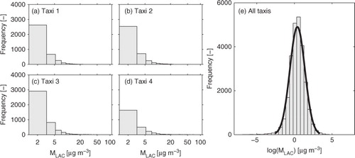
Table 1. M_LAC descriptive statistics for every taxi and all data together (1-min values), along with fixed site values (hourly data) in the period 7–17 November 2011

MLAC [µg m^−3]	Taxi 1	Taxi 2	Taxi 3	Taxi 4	All taxis	Hornsgatan	Torkel	Aspvreten
Arithmetic mean	2.3	2.3	2.5	3.0	2.4	3.3	0.9	0.3
Median	1.4	1.4	1.6	1.7	1.5	2.7	0.7	0.2
5th percentile	0.3	0.3	0.3	0.3	0.3	0.6	0.3	0.1
95th percentile	6.4	6.9	7.3	8.9	7.3	8.6	2.0	0.8
Maximum	103.9	80.2	48.6	69.0	103.9	16.0	3.8	1.3
Arithmetic SD	3.7	3.4	3.0	4.6	3.6	2.5	0.6	0.2
MAD	0.7	0.8	0.8	1.0	0.8	1.7	0.3	0.1
Skewness [–]	11.5	7.2	4.8	6.5	8.1	1.5	2.0	1.7
# samples	7080	7116	7107	4150	25 453	245	245	243

Compared to other urban experiments in Europe using mobile laboratories, our study revealed similar average concentrations. Mean M_LAC concentrations in Zurich ranged between 1.0 and 12.0 µg m⁻³, depending on the sampled sector (major traffic arteries, residential areas, suburbs, and surrounding hills) in 66 hours of winter campaigns (Mohr et al., 2011). In that case, traffic emissions were identified as a major contributor to LAC. Schneider et al. (2008) reported mean M_LAC values in the 1.5–9.4 µg m⁻³ range (depending on the road) for a mobile survey performed in Aachen inner city and outskirts during 7.5 hours in June 2005.

Stationary measurements in Stockholm showed higher values of M_LAC concentrations at the street canyon site, intermediate levels at the rooftop site, and lower levels always corresponded to the rural station. The 95th percentile at Hornsgatan was 10 times higher than the 95th percentile at Aspvreten, and the lowest values at Hornsgatan (5th percentile) are comparable to the 95th percentile at Aspvreten (0.6 µg m⁻³ vs. 0.8 µg m⁻³). These time series also exhibit a positive skewness and can be described by a lognormal distribution (not shown). These findings are in agreement with results from a previous campaign conducted in Stockholm in spring 2006 (Krecl et al., 2011).

In our study, concentrations gathered at fixed sites and mobile measurements have substantially different sampling frequency (hourly average vs. 1-min values) and totally different geographical representation. Note that drive-by measurements must be sampled with high frequency to resolve the spatial variability with enough detail. For instance, 1-min measurements represent 500 m for a vehicle driving at 30 km h⁻¹ whereas a vehicle driving at 90 km h⁻¹ travels 1500 m in the same time period. As previously mentioned, mobile platforms more accurately assess the pollution levels to which individuals are exposed in the short term compared to the hourly statistics (mean, maxima, etc.) usually reported by fixed monitoring stations. For example, while a fixed instrument at Hornsgatan site (street canyon) recorded a maximum hourly value of 16.0 µg m⁻³ for M_LAC on a given day, portable devices measured very high 1-min values at other locations in the city (e.g. peak values of 40–60 µg m⁻³ inside road tunnels, Fig. 9a, b). Even if the sampling time resolution increases at the stationary sites, they are not able to provide the spatial coverage offered by mobile surveys. This clearly remarks the importance of conducting highly-resolved mobile surveys to identify hotspots and support outdoor epidemiological studies at the intra-urban scale.

3.3. Temporal variation of M_LAC concentrations

Figure 3 shows the diurnal variation of hourly M_LAC concentrations (median and interquartile range) for the whole mobile dataset and at the three stations. Depending on the taxis operational scheme and fraction of invalid data, the number of 1-min samples included in the hourly calculation varied over the day (Fig. 3a), with fewer observations in the small hours (01:00–05:00). The hourly data coverage for the stationary measurements was between 99 and 100% (not shown).

Fig. 3 Diurnal variation of M_LAC concentrations (median: solid line, interquartile range: grey area) for all mobile measurements (a), and for three fixed stations (b) in the period 7–17 November 2011. Number of 1-min mobile samples included per hour for the diurnal calculation is also displayed.

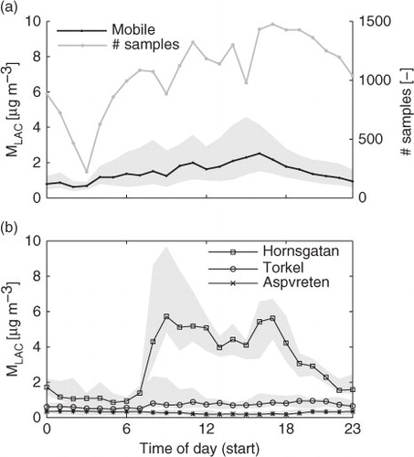
As regards fixed sites, M_LAC levels were always higher at the street canyon compared to the other sites, particularly during daytime. Measurements at the rural site (Aspvreten) were almost constant, indicating no evidence of local anthropogenic activities. These findings agree well with results from a previous campaign reported by Krecl et al. (2011). The rise in M_LAC levels observed at the urban stations in the early morning (06:00–07:00) is consistent with an increase in vehicle traffic and, thus, a larger contribution to the emissions (Krecl et al., 2011). Highest hourly values were observed during the morning at both urban sites, especially between 09:00 and 10:00. Peak levels were followed by a concentration decline at both stations through the afternoon, partially explained by the well-documented growth of the mixing layer depth and strong turbulent mixing during the afternoon. Urban background levels then remained quite flat until the end of the day, whereas a second peak value was observed at the street canyon station (16:00–18:00).

The mobile M_LAC measurements showed a gradual increase during the day, reached a maximum level in the late afternoon (16:00–17:00) and decreased afterwards. On average, similar levels as the ones monitored at the urban background station (Torkel) were recorded between 21:00 and 05:00. The distinct diurnal cycle of mobile measurements compared to the other site patterns might be explained by taxis driving during the day in city sectors characterised by different LAC contributions. We further investigate this possibility in Section 3.4.

Weekend (Saturday–Sunday) M_LAC concentrations accounted for 16% of the measurements and median values were statistically significantly lower than weekday values during the sampling period: 1.3 and 1.6 µg m⁻³, respectively (Mann–Whitney U test performed at 95% confidence level).

3.4. M_LAC concentrations, vehicle speed and traffic rates

Vehicle speed time series were averaged (median values) over 1-min intervals matching M_LAC concentrations, and tunnel measurements (1%) were excluded because of missing GPS signals. Then descriptive statistics were calculated for each taxi and the whole dataset (Table 2). Note that the total number of samples is lower than the number of mobile M_LAC measurements (Table 1) due to shorter battery life times for the GPS dataloggers, road tunnels exclusion, and cut-off distance introduced to integrate the different datasets. Despite the lower number of samples for taxi #4, almost all statistics agreed quite well with the results for the other datasets, especially with taxi #3. The lowest speed values (5th percentile) corresponded to periods when taxis were parked or stopped at traffic light intersections. High speeds (95th percentile) were recorded for all taxis and ranged between 90.7 and 104.3 km h⁻¹. As shown for M_LAC measurements, vehicle speed for individual taxis showed the same general pattern obtained for the composite dataset. All distributions presented positive skewness values (1.2–1.6).

Table 2. Vehicle speed descriptive statistics using 1-min median measurements for every taxi and all data together in the period 7–17 Nov 2011

Vehicle speed [km h^−1]	Taxi 1	Taxi 2	Taxi 3	Taxi 4	All taxis
Arithmetic mean	21.4	24.8	26.0	28.2	24.4
Median	5.9	12.4	13.7	17.9	11.7
5th percentile	0.1	0.1	0.1	0.1	0.1
95th percentile	90.7	100.4	104.3	100.3	99.2
Arithmetic SD	29.2	31.5	32.4	32.2	31.2
MAD	5.8	12.3	13.4	17.7	11.6
Skewness [–]	1.6	1.4	1.4	1.2	1.4
# samples	6109	5430	4807	2417	18 763

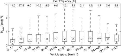
We classified temporally adjusted M_LAC concentrations according to their concurrent driving speed into 13 categories: 0–0.1 (vehicle parked or at traffic intersections), and 10 km h⁻¹ intervals up to 110 and >110 km h⁻¹ (highest speed permitted is 110 km h⁻¹ for the roads in the study area). Results presented in box-plot format (Fig. 4) show that the relationship between M_LAC concentrations and taxi speed was not linear. Highest M_LAC levels (median of 2.4 µg m⁻³ and 95th percentile of 11.0 µg m⁻³) and larger variability occurred for vehicle speeds in the 50–70 km h⁻¹ range, which accounted for 7% of the measurements.

Fig. 4 Box plots of M_LAC concentrations (temporally adjusted) classified by the corresponding vehicle speed in the period 7–17 November 2011. Box represents interquartile range and whiskers are lines that extend from the 5th to 95th percentile. Median is indicated by the line across the box and the cross marks the mean value. Percentages in the top line indicate the relative frequency of occurrence for each category.

To better understand the link between M_LAC levels and taxi speed, we analysed this relationship for every road type previously defined (Supplementary file). On highways, highest M_LAC concentrations (median of 3.8 µg m⁻³, and 95th percentile of 16.1 µg m⁻³) were observed for low taxi speeds (0.1–30 km h⁻¹) and then started to decrease. In the study region, the traffic regulation established a speed limit of 70 km h⁻¹ or above for a large fraction (85%) of the highway class. Thus, low taxi speed values might have been connected to highway transects with entry or exits, congestion at intersections with traffic lights and/or roundabouts that slowed down the traffic rate and decreased inter-vehicle distances, increasing the sampling of vehicle emissions. On the contrary, higher vehicle speeds increased inter-vehicle distances and, hence, favoured dilution prior to sampling. Main roads showed a similar trend, but M_LAC concentrations and taxi speeds were lower than on highways. The maximum speed allowed on the sampled main roads was 50 km h⁻¹ (79%) or even lower since main streets are located in the inner city where population density is high (3600 inhabitants km⁻²). When taxis were parked on the road or waiting at the intersections with traffic lights (0–0.1 km h⁻¹), median M_LAC concentrations were higher for main roads (1.2 µg m⁻³), but canyon streets presented the largest variability and highest 95th percentile (8.2 µg m⁻³). Idle engines in congested traffic areas can increase ambient concentrations and also increase the sampling of direct emissions since the inter-vehicle distance increases, as commented on before. The particular geometry of canyon streets might have also played a role in this aerosol accumulation process, reducing ventilation in case the wind was blowing perpendicular to the canyon axis. Local roads presented a completely different pattern in relation to M_LAC concentrations and vehicle speed when compared to other roads, with concentrations increasing with vehicle speed and peaking at 50–70 km h⁻¹. Median M_LAC values are statistically significantly different for taxi speeds between 0.1 and 60 km h⁻¹ when comparing local roads and highways (a Mann–Whitney U test was performed on the median difference concentration for each speed category at 95% confidence level). Local roads are narrower and have lower speed limits (30–50 km⁻¹) than highways, and are generally surrounded by buildings that can reduce ventilation. Due to the large number of data sampled on local roads (54%), their M_LAC pattern substantially contributed to the general M_LAC-speed relationship as depicted in Fig. 4. Analysing the traffic rates for local roads as a function of vehicle speed (not shown), the M_LAC distribution matched the hourly traffic rate pattern for speeds up to 70 km h⁻¹. This means that the traffic rate increased with vehicle speed, leading to higher M_LAC levels. Vehicle speeds higher than 70 km h⁻¹, increased the inter-vehicle distance even when traffic rates remained constant and, as a consequence, lowered the M_LAC levels on the road.

We cannot rule out the possibility of self-contamination when taxis drove at speeds lower than 5 km h⁻¹ (Weimer et al., 2009), however M_LAC values corresponding to the 0.1–10 km h⁻¹ interval were low when compared to concentrations of other speed categories.

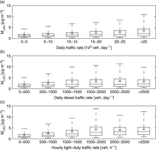
Finally, we analysed the relationship between temporally adjusted M_LAC concentrations and traffic rates, considering daily values for all vehicles and for the diesel fraction, and hourly rates for light-duty vehicles (Fig. 5). A clear increasing trend was observed for M_LAC levels with daily traffic rates as depicted in Fig. 5a, b. Note that, on a particular day and hour, daily traffic rates might vary widely from the annual average due to holidays, and day of the week. Thus, hourly traffic rates might be more representative of the real-world conditions since they were calculated taking into account diurnal variations of traffic volume for a particular hour, day of the week, month, and road type. Figure 5c shows a clear increase of M_LAC concentrations for light-duty vehicles on roads with traffic rates up to 2000 vehicles h⁻¹, which represented 89% of the cases. When traffic rates were higher, median and interquartile M_LAC concentrations remained almost constant, and the highest concentrations (95th percentile) slightly decreased. Considering the whole dataset, there is a substantial difference in median concentrations when comparing quite roads (1.1 µg m⁻³) with busy streets (3.3 µg m⁻³). Measurements segregated by road type also showed the same pattern (Supplementary file), and the largest difference in medians when comparing quiet and trafficked conditions corresponded to local roads (1.1 vs. 4.4 µg m⁻³). For the same volume of traffic, local roads presented higher M_LAC concentrations (median, 75th and 95th percentiles) than highways and this finding reinforces the idea previously discussed that local roads did not favour the pollution dispersion due to their narrower geometry and surrounding landscape.

Fig. 5 M_LAC concentrations as a function of traffic rates: (a) daily, all vehicles, (b) daily, diesel vehicles, and (c) hourly, gasoline vehicles in the period 7–17 November 2011. Represented are 5th, 25th, 50th, 75th, and 95 percentiles, and mean (x) values.

3.5. Spatiotemporal distribution

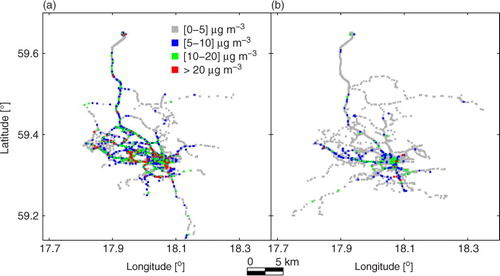
Based on the diurnal cycle study, georeferenced mobile measurements were classified as daytime (06:00–18:00)and night-time (18:00–06:00) data. After filtering to extract unique latitude-longitude coordinates, each coordinate location was mapped with associated M_LAC concentrations classified into four classes: 0–5, 5–10, 10–20, and >20 µg m⁻³ (Fig. 6). Median concentrations were higher during the day (1.9 µg m⁻³) than at night (1.2 µg m⁻³), varied widely depending on the street and time of the day, and appeared to be strongly influenced by traffic emissions as previously discussed. Our results agree with findings by Krecl et al. (2011), who reported a highly heterogeneous distribution of M_LAC concentrations in Stockholm when analysing measurements at four fixed sites. The highly-resolved pollution measurements, carried out with portable devices, can complement concentrations simulated by air quality dispersion models that usually do not capture this variability due to uncertainties in meteorology and emission inventories, complexity of the urban canopy and coarse spatial resolution.

Fig. 6 Spatial distribution of temporally adjusted M_LAC concentration in the Stockholm metropolitan area for (a) daytime (06:00–18:00), and (b) night-time (18:00–06:00) in the period 7–17 November 2011.

To better understand the spatial variability of M_LAC concentrations, measurements were classified according to the road type where they were sampled. Statistics of 1-min M_LAC levels (Table 3) and vehicle speed data for these sectors were calculated, along with hourly traffic rate per street group. Results were condensed in box-plots showing median, interquartile range, and 5th and 95th percentile values (Fig. 7). Since vehicle speed data for tunnels was not complete due to the large loss of GPS signals and we lacked detailed traffic rate for all tunnels, we do not present their statistics in Fig. 7. Stockholm road tunnels are part of important transportation arteries and their length varies between ~0.1 and 3.8 km, with traffic rates as high as 132 000 vehicles day⁻¹. Samples inside tunnels represented 1% of the measurements and showed the highest M_LAC concentrations in the metropolitan region: median, 5th and 95th percentile of 7.5, 0.9 and 40.1 µg m⁻³, respectively. This is expected as confined tunnel environments present a less efficient dispersion of atmospheric pollutants (e.g. Gidhagen et al., 2003). For the other four categories, the lowest concentrations were very similar (5th percentile of 0.3–0.5 µg m⁻³), and the variability between categories increased for higher concentrations (95th percentile was lowest for the local roads and highest for highways). Highways accounted for 21% of the measurements, and presented both the highest driving speeds (median of 65 km h⁻¹) and traffic rates (median of ~62 000 vehicles day⁻¹ and 1500 vehicles h⁻¹). The samples classified as highways in this study presented a larger share of diesel vehicles (69% of the samples have an annual mean diesel fraction of 7–10%) than local streets (64% of samples on roads with 4% share of diesel vehicles). Regardless of the vehicle speed and city sector, LAC emission factors are always higher for heavy duty vehicles compared to passenger and light duty vehicles (Keuken et al., 2012). Thus, the relatively high M_LAC levels found on highways could be explained by a more frequent sampling of exhaust plumes from diesel-powered vehicles driving at highway speed in front of the taxis and higher traffic volume. Canyon configurations are mostly found on main roads and presented slightly higher concentrations than main roads without canyon structure (medians are statistically different at 95% confidence level, Mann–Whitney U test).

Fig. 7 Boxplot of 1-min vehicle speed, daily (TR) and hourly (TRh) traffic rate, and 1-min M_LAC concentrations classified into four categories: local roads, street canyon, main roads, and highways in the period 7–17 November 2011. Represented are 5th, 25th, 50th, 75th, and 95 percentiles, and mean (x) values.

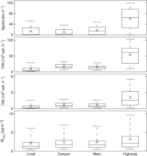
Table 3. Descriptive statistics (1-min values) of temporally adjusted M_LAC concentrations for five road types in the period 7–17 Nov 2011

MLAC (µg m^−3)	Tunnel	Highway	Main road	Canyon street	Local road
Arithmetic mean	12.9	3.2	2.4	2.4	2.1
Median	7.5	2.1	1.7	1.8	1.3
5th percentile	0.9	0.5	0.4	0.5	0.3
95th percentile	40.1	9.7	6.7	7.0	6.1
Arithmetic SD	13.8	3.7	3.1	2.4	3.3
MAD	5.1	1.2	0.8	0.8	0.7
# samples (%)	1	21	14	10	54

Unlike other studies (Yli-Tuomi et al., 2005; Schneider et al., 2008), we found mean M_LAC concentrations higher on highways (3.2 µg m⁻³) than on main roads (2.4 µg m⁻³), located in the inner city. Yli-Tuomi et al. (2005) reported an average value of 11 µg m⁻³ in Helsinki city centre compared to 8 µg m⁻³ on the surrounding highways. Schneider et al. (2008) found mean values of 9.4 µg m⁻³ in Aachen city – when sampling for 30 min during the morning and 7.9 µg m⁻³ during truck chasing on highways for approx. 5 hours. Westerdahl et al. (2005) measured higher M_LAC concentrations (median of 12–13 µg m⁻³) on highways (~10 000–25 000 diesel powered trucks per day) compared to residential areas (median of 0.7–1.5 µg m⁻³) in Los Angeles in a 4-d campaign in spring 2003. It is most likely that the values we report are lower than the concentrations observed by the other authors because we sampled for a longer time and included also night-time periods, which were characterised by lower pollution levels.

Even though the taxi roof measurements were not conducted along kerbsides, where people walk, they indicate large spatial variability in population exposure in traffic environments. As an example, M_LAC concentrations along a main road in the inner city (Sveavägen, Fig. 9c) varied from 3.1 to 25.1 µg m⁻³ (street median value of 5.9 µg m⁻³) in a weekday afternoon, with increasing values towards the city centre. These mobile observations also indicate a large variability for taxi drivers’ exposure while driving from less trafficked local streets to very polluted road tunnels. The in-vehicle exposure can be more or less attenuated in relation to the outdoor levels depending on the pollutants penetration efficiency.

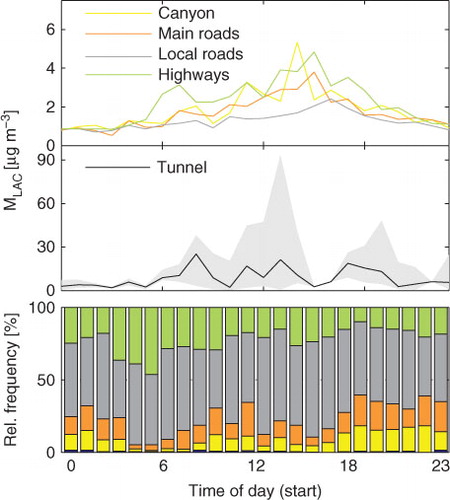
Figure 8 displays the diurnal variation of M_LAC concentrations (median values) for the five roadway groups, along with the relative frequency per hour for each street category. Due to the higher M_LAC concentrations, tunnel median measurements are presented in a separate panel, along with the 5th and 95th percentiles. Note that tunnel measurements were scarce, especially at certain hours of the day (02:00–07:00, 15:00–16:00, 22:00). This highlights the need for a dedicated campaign to better assess the M_LAC concentrations inside road tunnels, and actual drive-by measurements were conducted in Södra Länken (longest road tunnel in Stockholm) for several days in 2012 and will be published in a separate paper. The sampling frequency of different road groups was not the same over a whole day as depicted in Fig. 8 (bottom panel). Sampling of local roads was dominant along a whole day, with the highest frequency around midday. Measurements on canyons and main roads were more numerous at night (18:00–00:00), whereas taxis drove on highways more frequently in the early morning (03:00–07:00) and a first peak M_LAC value was observed at 07:00 matching very busy highways (median of 3400 vehicles h⁻¹). Highest M_LAC levels were recorded in the afternoon with the largest contribution from canyons and highways. Excluding tunnels, M_LAC concentrations were very similar at night (21:00–05:00, median of 0.9 µg m⁻³) on all roads when traffic rates were the lowest, and also compared with rooftop levels measured at Torkel site (Table 1). The diurnal pattern of M_LAC concentrations at the street canyon site (Hornsgatan) is very different from the daily variation from drive-by measurements on canyon streets during daytime. Several factors could have contributed to this distinct behaviour: not all sampled street canyons have the same geometry (aspect ratio, walls symmetry, canyon length) and street axis orientation (relevant for wind dispersion of pollutants), different sampling heights for mobile and fixed monitoring (inlets at 1.5 and 2.5 m height above the road surface, respectively), poor drive-by sampling in the street canyons in the morning when concentrations are highest according to Hornsgatan measurements, and mobile measurements were conducted along the street canyons (including intersections) whereas the fixed site is at ~70 m from a traffic-light intersection.

Fig. 8 Upper panel: Diurnal variation of M_LAC concentrations (median values) for four roadway groups (canyon, main roads, local roads, and highways) in the period 7–17 November 2011. Middle panel: Median (black line) and 5th to 95th percentile (grey area) M_LAC concentrations for tunnels in the same period. Bottom panel: Relative frequency per hour for each roadway group.

3.6. Case studies

To illustrate different driving cycles and pollution settings across the city, we show selected M_LAC concentrations and vehicle speed simultaneously measured during the field campaign (Fig. 9). As was previously presented, high concentrations were observed inside tunnels especially during daytime (Fig. 9a–b). Missing vehicle speed data corresponded to periods inside tunnels when the GPS signal was lost. The pollution level in a road tunnel depends, among other factors, on the tunnel length, vehicle fleet composition and speed, and traffic rate. A long driving time inside Södra Länken tunnel (3.8 km length, and 10-min passage) resulted in relatively large M_LAC values over several minutes whereas a shorter driving through Söderledstunneln (1.6 km length, 3 min.) recorded a higher and narrower peak concentration (59.8 µg m⁻³). On roads with traffic lights controlled intersections, M_LAC concentrations can be spiky during traffic peak hours due to higher emissions since many vehicles queue in idle mode at joins and, subsequently, accelerate. Figure 9c displays a transect mostly on Sveavägen street (16:32–16:42), driving towards the city centre with a mean vehicle speed of 10.8 km h⁻¹. The Sveavägen street transect was 1.8 km long with seven stops and an average stop duration of 35 sec. due to traffic lights. Because of this traffic control, concentrations exhibited a saw-tooth pattern reaching a maximum value of 25.1 µg m⁻³, influenced also by a street canyon effect in some sections (wind of 2.6 m s⁻¹ blowing at angle of more than 30° to the canyon axes, Vardoulakis et al., 2003).

Fig. 9 Case studies: 1-min M_LAC time series measured on board taxis together with vehicle speed: (a) Long driving inside Södra Länken tunnel (grey area). (b) Short driving inside Söderledstunneln tunnel (grey area). (c) Stop-and-go driving on Sveavägen street (inner city) due to traffic lights at several intersections, x indicates canyon structure. (d) Taxi parked on a local road very close to a hamburger grill. (e) High speed driving on E20 highway. (f) High speed driving on E4 highway.

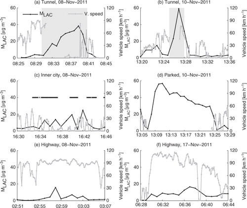
Usually M_LAC concentrations were low on local roads, as shown in section 3.5, but other LAC sources than tailpipe emissions can eventually dominate and drastically increase air pollution levels on a local scale. Figure 9d depicts M_LAC concentrations when the taxi was parked on a local street very close to a hamburger grill for a few minutes (13:07–13:24). In this case, we attributed the high and persistent M_LAC concentrations to emissions from charcoal combustion for meat cooking after Oanh et al. (1999) reported high particulate matter levels associated with charcoal combustion for cooking. High speed driving (>90 km h⁻¹) is illustrated in Fig. 9e–f when taxis circulated towards the city centre on E20 highway at night (traffic rate of 20–350 vehicles h⁻¹) and E4 highway in the early morning (4500–7200 vehicles h⁻¹), respectively. These examples show some sharp spikes, probably due to sampling behind diesel-powered vehicles driving at highway speed (Westerdahl et al., 2005; Schneider et al., 2008). Concentrations of M_LAC were higher and for a longer period during the daytime case, most likely because more vehicles were on the highway than in the small hours period. Since we found a large variability in M_LAC concentrations when looking at individual cases, we stress the importance of performing a spatiotemporal analysis to summarise and better understand this variability across the city.

Based on these results, we should assess whether or not the M_LAC monitoring air pollution network, composed of stationary stations, in the Stockholm metropolitan region is optimised in terms of spatial coverage. In light of the geographical variability shown by the mobile survey, even on the same street (Fig. 9c), the representativeness of the fixed stations is questionable. Such M_LAC variability is more important for the highest concentrations, and thus for the short-term exposure of the population, and less important for the long-term mean values (which is more dependent on traffic volume variations along a street). Ambient air quality standards in Europe do not include LAC concentrations yet, but there are specific air quality directives for monitoring other atmospheric pollutants at fixed sites (Directive EC, 2008) stating where and how measurements should be conducted. However, from the view point of population exposure, the directives might not indicate the best monitoring locations as illustrated by the taxi data.

3.7. Multiple regression modelling

A pool of numerical and categorical variables was analysed to identify possible predictors of on-road M_LAC concentrations. Note that tunnel measurements were not included in the multiple regression since traffic rates were not available for this category. Table 4 displays the correlation matrix (Pearson) of the numerical variables: daily traffic rate (TR), hourly light-duty traffic rate (TRh), daily diesel traffic rate (TRd), road speed limit (RS), vehicle speed (VS), hourly M_LAC concentrations at the fixed sites (Hornsgatan, Torkel, and Aspvreten), hourly meteorological measurements conducted at Torkel (temperature T, relative humidity RH, wind speed WS and atmospheric pressure P) and population density (Pop). The highest correlation with the dependent variable corresponded to TRh (r=0.29), and we discarded TR and TRd as candidate variables since they are in the same category (traffic) and are highly correlated with TRh (r>0.6). All traffic rate variables have an impact on mobile M_LAC concentrations, but the similarity of their effect (high collinearity) dictates that only one of them is needed in the prediction process. For the same reason, only VS is kept in the model and RS is omitted. M_LAC concentrations at Hornsgatan and Torkel contribute to mobile M_LAC, and they are correlated between them (r=0.6). Population, atmospheric pressure, and M_LAC at Aspvreten were not considered since they showed a very low contribution to the explained variance of mobile M_LAC. We also include two sets of dummy variables: road type (highway, main roads, and canyon streets all relative to local roads), and time (weekdays during the day 06:00–18:00 LT and weekdays at night 18:00–06:00 LT, both relative to weekends). To remedy the lack of normality and improve homoscedasticity, a logarithmic transformation was applied to all M_LAC concentrations (i.e. mobile and fixed-site) and TRh.

Table 4. Correlation matrix between mobile M_LAC and numerical independent variables, with r>0.60 displayed in bold

r[–]	TR	TRd	TRh	RS	VS	MLACH	MLACT	MLACA	T	RH	WS	P	Pop
TRd	0.92
TRh	0.76	0.76
RS	0.69	0.74	0.58
VS	0.53	0.62	0.47	0.72
MLACH	−0.05	−0.03	0.23	−0.02	−0.02
MLACT	−0.03	−0.03	0.09	−0.02	−0.02	0.60
MLACA	0.03	0.02	0.00	0.03	0.03	0.26	0.66
T	0.01	0.00	0.06	0.01	−0.02	0.55	0.36	0.29
RH	0.04	0.04	−0.12	0.02	0.04	−0.50	−0.14	0.05	−0.56
WS	0.02	0.03	0.03	0.00	0.00	−0.12	−0.36	−0.03	−0.03	−0.04
P	−0.05	−0.02	−0.03	−0.03	0.03	−0.16	−0.08	−0.39	−0.45	0.48	−0.48
Pop	−0.17	−0.21	−0.15	−0.29	−0.26	−0.04	0.00	−0.02	−0.02	0.04	0.01	0.03
MLAC	0.17	0.16	0.29	0.12	0.13	0.27	0.20	0.01	0.13	−0.16	−0.09	0.02	−0.02

The model including a bilinear moderator presented the highest adjusted R ² (0.25) and smallest RMSE (0.82), and predicted the 1-min concentrations of on-road M_LAC on weekdays during the day [eq. (1 )] and on weekdays at night and weekends [eq. (2)]. More details on the model runs can be found in the Supplementary file.1 2

The most impactful predictor was log(TRh), closely followed by log(M_LACT). From an explanatory point of view, there are two main sources of on-road LAC in the urban area: local emissions from motorised vehicles (portrayed by hourly traffic rates) and a city build-up term (represented by the Torkel baseline values), and wind speeds act as a mixing factor between these two contributions. On weekdays during the day the on-road M_LAC concentrations depend on the hourly traffic rate on that road, and the hourly M_LAC concentration and wind speed measured at an urban background site. At night on weekdays and on weekends, the hourly traffic rate is not relevant and the on-road concentration is determined by the background conditions. This matches with our previous finding that night-time concentrations were very similar to Torkel levels for all road types in connection with low traffic volumes. The negative sign of the wind term represents the dilution of pollutants by the wind, and this effect increases with wind speed.

The residual analysis revealed the residuals are not normally distributed and are temporally (Supplementary file) and spatially autocorrelated (Moran's index of 0.24, p=0). By applying different diagnostics, 19% of the observations were identified as influential observations (Supplementary file). When these outliers were excluded from the dataset, the same regression equation explained now 34% of the variance observed in the mobile M_LAC concentrations and the RMSE was smaller (0.61 vs. 0.82). The fact that the model was not able to represent the extremely local variations in concentrations, even when the outliers were removed, suggest a highly non-linear problem that cannot be properly modelled with just including a bilinear moderator.

The estimation of the model robustness was based on 300 runs with random removal of 25% of the original dataset, producing RMSE values between 0.80 and 0.87 (mean of 0.83), and adjusted R² values between 0.19 and 0.26 (mean of 0.23). The selected variables by the stepwise method were log(TRh), log(M_LACT), RH, WS, and weekday-day, but only log(TRh) and log(M_LACT) were present in all regression equations, which matches with our previous finding that these variables are the most impactful when predicting on-road M_LAC concentrations.

4. Summary and conclusions

To map out atmospheric pollutants in urban areas, rolling platforms provide a larger spatial coverage than a network of stationary monitoring sites, and can be used either for stationary or drive-by measurements. This work reports on the first mobile M_LAC concentrations measured in the Stockholm metropolitan area, collecting 424 hours of valid data in multiple trips covering ~7600 km of metropolitan roads. Simultaneous M_LAC measurements were conducted both with Micro Aethalometers on-board four taxis (1-min resolution) and custom-built PSAPs installed at three fixed stations (hourly values). Individual datasets per taxi captured the grand statistical pattern made up by the drive-by composite measurements, with median and MAD M_LAC concentrations ranging from 1.4 to 1.7 µg m⁻³, and from 0.7 to 1.0 µg m⁻³, respectively. On-road daytime concentrations were higher and more variable than night-time levels, and concentrations at night were independent of the road type and similar to the urban background levels (median of 0.9 µg m⁻³). The relationship between M_LAC levels and vehicle speed was not linear, and peak concentrations varied depending on the road type. Highways presented the highest concentrations for low taxi speeds (0.1–30 km h⁻¹) when roads were busy and inter-vehicle distances smaller, and the same general trend was observed for main roads and urban canyons (mostly located on main roads). Differently, concentrations on local roads increased with vehicle speed up to 50–70 km h⁻¹, associated with increasing hourly traffic rate and poorer ventilation due to smaller width and surrounding structure.

A large variability in concentrations was observed along the different roads, with maxima levels inside road tunnels (median and 95th percentile of 7.5 and 40.1 µg m⁻³, respectively). Highways presented the second highest concentrations (median and 95th percentile of 3.2 and 9.7 µg m⁻³, respectively) and were associated with highest vehicle speed, traffic rates, and diesel vehicles share. Measurements on canyon streets were slightly higher than levels recorded on main roads, most likely connected to lower atmospheric dispersion in urban canyons.

Even though multiple regression is just a statistical technique and the model explained only 25% of the variance observed in on-road M_LAC concentrations, the regression variate identified the best predictor variables (hourly traffic rate, and M_LAC concentrations at a urban background site) and roughly explained the physics of the problem. In that sense, we discourage using the regression equations for prediction purposes.

This feasibility study represents a step forward in characterising the spatiotemporal variability of M_LAC concentrations in the Stockholm metropolitan area by using a limited amount of sensors and platforms that proved to be a time- and cost-effective approach. However, there are some limitations to our experimental method that could be improved in future campaigns. Due to the lack of video recording, we had no information on possible pollution plumes emitted by vehicle driving on the same road and sampled by our instruments, and it was more time consuming to identify road changes (e.g. transects within tunnels and traffic lights stops at intersections) and also discard invalid data. The derived spatiotemporal distribution of M_LAC concentrations only reflects the conditions when we conducted the measurements and further field experiments are required to represent the M_LAC distribution in other periods of the year (i.e. change in emission patterns, and different dispersion conditions under other meteorological settings). Future field campaigns should monitor other important pollutants using portable devices, most notably nitrogen oxides, which were found to be closely correlated with M_LAC concentrations (Krecl et al., 2011) in traffic-related environments and could be used to better identify the LAC emission sources.

In light of the geographical M_LAC variability shown by this mobile survey, even on the same street, the representativeness of the fixed stations is questionable from the viewpoint of population exposure assessment.

5. Acknowledgements

The Environmental Fund of the Stockholm County Administration, the Norwegian Research Council and the Arctic Earth Observatory project supported this work. Taxi Stockholm is acknowledged for providing the four taxis to conduct the mobile measurements, and Wangzhang Wei for assistance during the measurement campaign.

Notes

To access the supplementary material to this article, please see Supplementary files under Article Tools online.

References

- Attfield M. D , Schleiff P. L , Lubin J. H , Blair A , Stewart P. A , co-authors . The diesel exhaust in miners study: a cohort mortality study with emphasis on lung cancer. J. Natl. Cancer. Inst. 2012; 104: 869–883.
- Bond T. C , Doherty S. J , Fahey D. W , Forster P. M , Berntsen T , etal. Bounding the role of black carbon in the climate system: a scientific assessment. J. Geophys. Res. 2013; 118: 5380–5552.
- Directive 2008/50/EC of the European Parliament and of the Council of 21 May 2008 on ambient air quality and cleaner air for Europe. Tech. Rep. Off. J. Eur. Comm. L152: 1–44.
- Dons E , Int Panis L , Van Poppel M , Theunis J , Wets G . Personal exposure to black carbon in transport microenvironments. Atmos. Environ. 2012; 55: 392–398.
- Draxler R. R , Rolph G. D . HYSPLIT (HYbrid Single-Particle Lagrangian Integrated Trajectory). 2013. NOAA Air Resources Laboratory, Silver Spring, MD.
- Gidhagen L , Johansson C , Ström J , Kristensson A , Swietlicki E , co-authors . Model simulation of ultrafine particles inside a road tunnel. Atmos. Environ. 2003; 37: 2023–2036.
- Hair J. F , Tatham R. L , Anderson R. E , Black W . Multivariate Data Analysis. 1998. 5th ed. Prentice Hall International, London.
- Hansson H.-C , Christer J , Nyqvist G , Kindbom K , Åström S , etal. Black carbon – possibilities to reduce emissions and potential effects. Tech. Rep. ITM. 2011; 202: 1–64. Online at: http://slb.nu/slb/rapporter/pdf8/itm2011_202.pdf .
- Henderson S , Beckerman B , Jerret M , Brauer M . Application of land use regression to estimate long-term concentrations of traffic-related nitrogen oxides and fine particulate matter. Environ. Sci. Technol. 2007; 41: 2422–2428.
- Janssen N. A. H , Gerlofs-Nijland M. E , Lanki T , Salonen R. O , Cassee F , etal., Bohr R . Health Effects of Black Carbon. 2012; Copenhagen: WHO Regional Office for Europe. 1–86. Online at: http://www.unece.org/fileadmin/DAM/env/lrtap/conv/Health_Effects_of_Black_Carbon_report.pdf .
- Johansson C , Eneroth K . Traffic emissions, socioeconomic valuation and socioeconomic measures. Stockholm and Uppsala Air Quality Association. Tech. Report LVF. 2007. 2007(2), 1–22. Online at: http://www.slb.nu/slb/rapporter/pdf8/lvf2007_002.pdf .
- Keuken M. P , Jonkers S , Zandveld P , Voogt M , Elshout van den S . Elemental carbon as an indicator for evaluating the impact of traffic measures on air quality and health. Atmos. Environ. 2012; 61: 1–8.
- Krecl P , Johansson C , Ström J . Spatiotemporal variability of light-absorbing carbon concentration in a residential area impacted by woodsmoke. J. Air Waste Manage. 2010; 60: 356–368.
- Krecl P , Ström J , Johansson C . Carbon content of atmospheric aerosols in a residential area during the wood combustion season in Sweden. Atmos. Environ. 2007; 41: 6974–6985.
- Krecl P , Targino A. C , Johansson C . Spatiotemporal distribution of light-absorbing carbon and its relationship to other atmospheric pollutants in Stockholm. Atmos. Chem. Phys. 2011; 11: 11553–11567.
- Mohr C , Richter R , DeCarlo P. F , Prévôt A. S. H , Baltensperger U . Spatial variation of chemical composition and sources of submicron aerosol in Zurich during wintertime using mobile aerosol mass spectrometer data. Atmos. Chem. Phys. 2011; 11: 7465–7482.
- Norlin L . Dataproduktspecifikation – Det svenska vägnätet, Version1.0. 2013. Trafikverket. Online at: http://www.trafikverket.se/TrvSeFiler/Foretag/Bygga_och_underhalla/Vag/Dataproduktionspecifikationer/Trafiknat/Vag/DPS_Vagnat_1.pdf (only in Swedish).
- Norman M , Johansson C . Studies of some measures to reduce road dust emissions from paved roads in Scandinavia. Atmos. Environ. 2006; 40: 6154–6164.
- Noth E. M , Hammond S. K , Biging G. S , Tager I. B . A spatial–temporal regression model to predict daily outdoor residential PAH concentrations in an epidemiologic study in Fresno, CA. Atmos. Environ. 2011; 45: 2394–2403.
- Oanh N. T. K , Reutergardh L. B , Dung N. T . Emission of polycyclic aromatic hydrocarbons and particulate matter from domestic combustion of selected fuels. Environ. Sci. Technol. 1999; 33: 2703–2709.
- Pirjola L , Parviainen H , Hussein T , Valli A , Hämeri K , co-authors . “Sniffer” – a novel tool for chasing vehicles and measuring traffic pollutants. Atmos. Environ. 2004; 38: 3625–3635.
- Schneider J , Kirchner U , Borrmann S , Vogt R , Scheer V . In situ measurements of particle number concentration, chemically resolved size distributions and black carbon content of traffic-related emissions on German motorways, rural roads and in city traffic. Atmos. Environ. 2008; 42: 4257–4268.
- Silverman D. T , Samanic C. M , Lubin J. H , Blair A. E , Stewart P. A , co-authors . The diesel exhaust in miners study: a nested case–control study of lung cancer and diesel exhaust. J. Natl. Cancer. Inst. 2012; 104: 855–868.
- Statistics Sweden . Population Statistics 2012. 2012. Online at: http://www.scb.se/Pages/TableAndChart____350653.aspx .
- Thornhill D. A , de Foy B , Herndon S. C , Onasch T. B , Wood E. C , co-authors . Spatial and temporal variability of particulate polycyclic aromatic hydrocarbons in Mexico City. Atmos. Chem. Phys. 2008; 8: 3093–3105.
- Tunved P , Hansson H. C , Kulmala M , Aalto P , Viisanen Y , co-authors . One year boundary layer aerosol size distribution data from five Nordic background stations. Atmos. Chem. Phys. 2003; 3: 2183–2205.
- Unger N , Bond T. C , Wang J. S , Koch D. M , Menon S , co-authors . Attribution of climate forcing to economic sectors. Proc. Natl. Acad. Sci. U. S. A. 2010; 107: 3382–3387.
- Vardoulakis S , Fisherb B. E. A , Pericleous K , Gonzalez-Flescac N . Modelling air quality in street canyons: a review. Atmos. Environ. 2003; 37: 155–182.
- Virkkula A , Mäkela T , Hillamo R , Yli-Tuomi T , Hirsikko A , co-authors . A simple procedure for correcting loading effects of Aethalometer data. J. Air Waste Manage. 2007; 57: 1214–1222.
- Wallace J , Corr D , Deluca P , Kanarogloua P , McCarry B . Mobile monitoring of air pollution in cities: the case of Hamilton, Ontario, Canada. J. Environ. Monit. 2009; 11: 998–1003.
- Wang M , Zhu T , Zheng J , Zhang R. Y , Zhang S. Q , co-authors . Use of a mobile laboratory to evaluate changes in on-road air pollutants during the Beijing 2008 Summer Olympics. Atmos. Chem. Phys. 2009; 9: 8247–8263.
- Wang X , Westerdahl D , Wu Y , Pan X , Zhang K. M . On-road emission factor distributions of individual diesel vehicles in and around Beijing, China. Atmos. Environ. 2011; 45: 503–513.
- Weimer S , Mohr C , Richter R , Keller J , Mohr M , co-authors . Mobile measurements of aerosol number and volume size distributions in an Alpine valley: influence of traffic versus wood burning. Atmos. Environ. 2009; 43: 624–630.
- Westerdahl D , Fruin S , Sax T , Fine P. M , Sioutas C . Mobile platform measurements of ultrafine particles and associated pollutant concentrations on freeways and residential streets in Los Angeles. Atmos. Environ. 2005; 39: 3597–3610.
- Yli-Tuomi T , Aarnio P , Pirjola L , Makela T , Hillamo R , co-authors . Emissions of fine particles, NOx, and CO from on-road vehicles in Finland. Atmos. Environ. 2005; 39: 6696–6706.