Processes limiting the emergence of detectable aerosol indirect effects on tropical warm clouds in global aerosol-climate model and satellite data

Abstract

We use data from simulations performed with the global aerosol-climate model ECHAM5-HAM to test the proposition that shipping emissions do not have a statistically significant effect on water clouds over tropical oceans on climate scales put forward in earlier satellite based work. We analyse a total of four sensitivity experiments, three of which employ global shipping emissions and one simulation which only employs shipping emissions in the mid-Atlantic Ocean. To ensure comparability to earlier results from observations, we sample the model data using a method previously applied to satellite data aimed at separating ‘clean’ from ‘polluted’ oceanic regions based on i) the location of main shipping routes and ii) wind direction at 10 m above sea level. The model simulations run with realistic present-day shipping emissions show changes in the lower tropospheric aerosol population attributable to shipping emissions across major shipping corridors over tropical oceans. However, we find the resulting effect on cloud properties to be non-distinguishable from natural gradients and variability, that is, gradients of cloud properties sampled across major shipping corridors over tropical oceans are very similar among those simulations. Our results therefore compare well to the earlier findings from satellite observations. Substantial changes of the aerosol population and cloud properties only occur when shipping emissions are increased 10-fold. We find that aerosol advection and rapid aerosol removal from the atmosphere play an important role in determining the non-significant response in i) column integrated aerosol properties and ii) cloud microphysical properties in the realistic simulations. Additionally, high variability and infrequent occurrence of simulated low-level clouds over tropical oceans in ECHAM5-HAM limit the development of aerosol indirect effects because i) in-cloud production of sulphate from ship-emitted sulphuric species via aqueous oxidation pathways is very low and ii) a possible observational signal is blurred out by high variability in simulated clouds. Our results highlight i) the importance of adequately accounting for atmospheric background conditions when determining climate forcings from observations and ii) the effectiveness of buffering mechanisms on micro- and macroscopic scales which limit the emergence of such climate forcings.

• aerosol indirect effects
• climate modelling
• aerosol microphysics
• parameterization
• cloud parameterization
• remote sensing
• geoengineering

To access the supplementary material to this article, please see Supplementary files under Article Tools online.

1. Introduction

Aerosol indirect effects (AIEs, Stevens and Feingold, 2009, and references therein) continue to contribute substantial uncertainty to estimates of the anthropogenic radiative forcing (RF) of the climate system (Boucher et al., 2013; Myhre et al., 2013). Understanding ambiguities associated with the quantification of AIEs from observations or numerical modelling can be accelerated by combining both methodologies (Quaas et al., 2009, 2010; Grandey et al., 2013). In this study, we analyse numerical simulations of AIEs from shipping emissions over global oceans by applying a methodology proven useful in an observational study of these AIEs (Peters et al., 2011) to investigate the underlying processes and associated uncertainties of aerosol–cloud interactions.

To access the supplementary material to this article, please see Supplementary files under Article Tools online

AIEs from shipping emissions, be it their manifestation in ship-tracks or their influence on large-scale cloud fields, have, over the past five decades or so, spawned a wealth of scientific studies utilising both observational (e.g. Conover, 1966; Coakley et al., 1987; Durkee et al., 2000b; Christensen and Stephens, 2011; Peters et al., 2011; Chen et al., 2012; Goren and Rosenfeld, 2012) and modelling (e.g. Capaldo et al., 1999; Lauer et al., 2007; Wang and Feingold, 2009; Righi et al., 2011; Lund et al., 2012; Peters et al., 2012, 2013; Partanen et al., 2013) approaches. While ship-tracks are one of the most prominent manifestations of AIEs, they mainly occur in stratocumulus cloud fields over mid-latitudes (e.g. Campmany et al., 2009), require specific environmental conditions to form (Durkee et al., 2000a) and thus yield negligible RF at the top of the atmosphere (TOA) (Schreier et al., 2007). As shipping emissions substantially modify the composition of the marine boundary layer (MBL) aerosol population (e.g. Matthias et al., 2010; Coggon et al., 2012) and often occur in otherwise pristine areas with potentially high cloud-albedo susceptibility to aerosol perturbations (Twomey et al., 1968; Platnick and Twomey, 1994), AIEs from shipping emissions can be expected to have a non-negligible impact on large-scale cloud fields – an assertion supported by results from global modelling which yield values of globally averaged AIEs ranging from −0.6 Wm⁻² to −0.07 Wm⁻² (Lauer et al., 2007; Righi et al., 2011; Peters et al., 2012, 2013; Partanen et al., 2013). Depending on the estimate, AIEs from shipping could thus make up for a substantial part of total globally averaged AIEs, with the current best estimate being −0.45 (−1.2 to 0.0) Wm⁻² (Myhre et al., 2013). Shipping emissions also lead to a considerable increase of long-lived greenhouse gas (GHG) concentrations in the atmosphere and shipping emission induced changes of atmospheric chemistry are substantial (cf. Isaksen et al., 2009, for a review). However, the large AIEs from shipping emissions dominate over the warming induced by the emitted GHGs, resulting in a net cooling of the climate system. Over the course of the next century, this is most likely to switch to a net warming effect if GHG emissions from ships continue to increase as expected and fuel sulphur content regulations take effect in the near future (Fuglestvedt et al., 2009).

Extracting the impact of shipping emissions on large-scale cloud fields on climatically relevant temporal scales from observational data has proven difficult (Devasthale et al., 2006; Peters et al., 2011), most likely due to i) limitations of satellite retrieval methods to quantify low-cloud properties over regions of high shipping emissions, such as in multi-layered cloud systems over mid-latitudes and ii) high natural variability resulting in low signal-to-noise ratios.

Here, we analyse a set of global aerosol climate model simulations very similar to the ones analysed in detail in previous work (Peters et al., 2012, P12 hereafter) and (Peters et al., 2013, P13 hereafter) to test the findings gained from satellite-based observations presented in (Peters et al., 2011, P11 hereafter) from another angle. P11, using satellite data from passive sensors spanning the time period of 2005–2007, did not find statistically significant effects of shipping emissions on water cloud micro- and macrophysical properties and atmospheric radiation. They constrained their analysis to shipping corridors over tropical oceans to enable separation of ‘clean’ and ‘polluted’ environments (with respect to shipping emissions). P11 concluded that ‘… the net indirect effects of aerosols from ship emissions are not large enough to be distinguishable from the natural dynamics controlling cloud presence and formation …’. Indeed, cloud radar observations show that relatively small fluctuations () in ambient meteorological conditions (relative humidity in this case) can lead to similar changes in trade-wind cumulus water content as a doubling of cloud droplet number concentrations (CDNC) (K. Lonitz, personal communication, 2014). P12 used the aerosol-climate model ECHAM5-HAM to estimate AIEs from shipping emissions and analyse the model's sensitivity towards uncertainties associated with the emission parameterisation as well as with the shipping emissions themselves. The model used prescribed SSTs and the dynamics were nudged to reanalysis data. AIEs were found to range from −0.45±0.02 to −0.08±0.01 Wm⁻² (P13), with more realistic estimates being rather on the more negative than positive side. Comparing the results of the above-mentioned studies, the question that immediately arises is:

Given the constrained setup of the model simulations presented in P12 and P13, can a statistically significant effect of shipping emissions on water clouds in the vicinity of tropical shipping corridors be extracted from the model data when the same sampling methodology as in P11 is applied?

Whatever the answer to this question turns out to be, analysis of the model data on such relatively small scales (from the perspective of climate modelling) also acts as a testbed for evaluating the cumulative effect of the parameterised microphysical and dynamical processes at the grid scale. For the case of water clouds over tropical oceans, such an analysis is also especially appealing because current generation GCMs do a poor job at representing observations (e.g. Nam et al., 2012) and because revisiting and improving parameterisations of cloud microphysics has been shown key to ameliorated water–cloud representation in atmospheric models (e.g. Franklin, 2008; Abel and Boutle, 2012; Weber and Quaas, 2012).

To answer the above question and to delve into the underlying processes parameterised in the model, we apply the sampling approach presented in P11 to the model simulations. That sampling approach is tailored towards separating regions upwind (‘clean’) of main shipping corridors from those downwind (‘polluted’), thereby testing the assumption that there exist statistically significant differences in large scale aerosol- and cloud properties between those two regions on climatically relevant scales. Complementary to the model setups used in P12, we also use results from a model simulation with unrealistically high shipping emissions and from a model simulation with local shipping emissions in the mid-Atlantic Ocean only.

The paper is structured as follows: in Section 2, we introduce the model setup and analysis strategy. Results which are directly comparable to those presented in P11 are presented in Section 3 and further analysis of spatial aerosol distributions is shown in Section 4. We summarise and discuss the results of our study in Section 5.

2. Modelling and analysis approach

2.1. Model setup

Using satellite observations, P11 found no statistically significant large-scale effect of shipping emissions on liquid-clouds over tropical oceans. Here, we apply the same sampling approach presented in that observational study to a set of simulations performed with the aerosol climate model ECHAM5-HAM presented in P12 and P13.

In the simulations discussed here, cloud cover is computed following a relative humidity-based approach (Sundqvist et al., 1989) and the treatment of convective clouds and transport is based on the mass-flux scheme of Tiedtke (1989). Stratiform cloud microphysics is computed according to Lohmann et al. (2007) with some description given below. Transport of physical quantities in gridpoint-space is performed via a semi-Lagrangian transport scheme (Lin and Rood, 1996).

In terms of aerosol representation in the model, ECHAM5 is coupled to HAM, a microphysical aerosol module which calculates the evolution of an aerosol population represented by seven interacting internally and externally mixed log-normal aerosol modes [Stier et al. (2005), with recent developments and remaining shortcomings documented in Zhang et al. (2012)]. In the setup used, HAM treats sulphate (SU), black carbon (BC), organic carbon [OC, further represented by particulate organic matter (POM)], sea salt (SS) and dust (DU) aerosol. The microphysical interaction among the modes, such as coagulation, condensation of sulphuric acid on the aerosol surface, and water uptake are calculated by the microphysical core M7 (Vignati et al., 2004). New particle formation is calculated as in the simulations of Kazil et al. (2010) (using ECHAM5-HAM): particle formation via (1) cluster activation and (2) neutral- and charged activation are treated following Kulmala et al. (2006) and Kazil and Lovejoy (2007), respectively. Further, HAM treats emissions, sulphur chemistry (Feichter et al., 1996), dry and wet deposition and sedimentation and is coupled to radiative processes.

Cloud microphysical properties are derived using a double-moment scheme, which solves prognostic equations for cloud water and ice mass mixing ratios as well as for the number of cloud droplets and ice crystals (Lohmann et al., 2007). Cloud droplet nucleation is parametrised as an empirical function of aerosol number concentrations (Lin and Leaitch, 1997) and Köhler theory based CCN diagnostics are also included. Autoconversion, that is, conversion from cloud droplets to form precipitation, is treated according to Khairoutdinov and Kogan (2000). Therefore, ECHAM5-HAM enables us to estimate AIEs of the first and second kind. Nam and Quaas (2012) evaluated the representation of clouds and precipitation in ECHAM5 using satellite observations and found that the model underestimates tropical and subtropical low-level cloud cover. However, the model is able to place these clouds in locations consistent with observations which is why we are confident that ECHAM5 is a useful tool for studying AIEs on oceanic low-level clouds.

The emissions of DU (Tegen et al., 2002), SS (Guelle et al., 2001) and dimethyl sulphide (DMS, Kettle and Andreae, 2000) are computed on-line. The emissions of carbonaceous and sulphuric compounds, except those from shipping, are prescribed according to the AeroCom (Kinne et al., 2006) recommendations (for the year 2000, Dentener et al., 2006). Gaseous species (e.g. OH, NO _X , ozone) are prescribed as monthly values after Horowitz et al. (2003).

We substitute the AeroCom shipping emissions (EDGAR, Bond et al., 2004; Olivier et al., 2005) with a dataset produced within the European Integrated Project QUANTIFY (EU-IP QUANTIFY), which comprises globally gridded data of shipping emissions for the year 2000 (Behrens, 2006). To distribute the annual emissions in the QUANTIFY inventory, marine reports from the COADS (Comprehensive Ocean–Atmosphere Data Set) and AMVER (Automatic Mutual-Assistance Vessel Rescue System) datasets at 1°×1° resolution were used for deriving global ship reporting frequencies as illustrated in Endresen et al. (2003). The global distributions are shown in Dalsøren et al. (2009). We acknowledge that incorporating shipping emissions at such spatial scales into a GCM introduces unrealistic dilution effects and neglects in-plume aerosol processes. Parameterisations of in-plume emission processing do exist (Franke et al., 2008; Stevens and Pierce, 2013) – employing such a parameterisation is however beyond the scope of this study. In the QUANTIFY inventory, the total annual fuel consumption is estimated at 172.5 Mt in the year 2000 which is substantially lower than the estimates of Corbett and Koehler (2003) and Eyring et al. (2005), being 289 Mt and 280 Mt, respectively. This difference in total annual fuel consumption has been a matter of debate and is attributed to different assumptions of ship activity levels (Corbett and Koehler, 2004; Endresen et al., 2004). The QUANTIFY inventory comprises annual emission sums of a variety of substances, we only consider emissions of SO₂, BC and OC, though.

The simulations are performed with a horizontal resolution of 1.8×1.8° (T63) and 31 vertical levels and monthly mean sea surface temperatures and sea ice cover are prescribed according to the AMIP II dataset (Atmospheric Model Intercomparison Project; Taylor et al., 2000). Here, ECHAM5-HAM is used in nudged mode to relax the prognostic variables (vorticity, divergence, temperature and surface pressure) towards reanalysis data (ERA-Interim, Simmons et al., 2007) and the simulations span the time period October 1999 to December 2004. The first 3 months are considered as model spin-up and the analysis is then performed on the remaining 5 yr.

In total, we investigate three sensitivity simulations (A, Bsc and Bsc10) addressing different aspects of uncertainties in the shipping emissions (see below), one simulation with shipping emissions in the mid-Atlantic Ocean only (Bsc_mAt) and one control simulation (CTRL) without any shipping emissions.

In model setup A, the shipping emissions are incorporated into the model environment as prescribed by AeroCom, that is, 2.5% of sulphur mass is emitted as particulate SU. Of this particulate SU, 50% is assigned to the soluble accumulation mode (number mean radius m, standard deviation σ=1.59) and 50% is assigned to the soluble coarse mode (m, σ=2). BC and OC are both assigned to the insoluble Aitken mode (m, σ=1.59).

In model setup Bsc, the emission attribution is changed compared to A so that 4.5% of sulphur mass is emitted as particulate SU completely assigned to the soluble Aitken mode. BC and OC are also completely assigned to the soluble Aitken mode. We applied these modifications because the original formulation as proposed in AeroCom and used in A severely contradicts observed properties of ship-emitted (cf. P12 for details) and industrially emitted particles in general (Stevens et al., 2012). Furthermore, the annual emissions are scaled by a factor of 1.63 to meet the highest published emission estimates for the year 2000 (Corbett and Koehler, 2003). Compared to A, the number of emitted soluble particles increases from s⁻¹ to s⁻¹. In the model setup Bsc_mAt, we only use those shipping emissions attributed to the area enclosed by top-left and bottom-right coordinate-pairs of 25N, 32W and 5S, 20W, respectively.

In model setup Bsc10, the emission attribution is the same as in Bsc, with the annual emissions scaled by a factor of 10 compared to A, thus perturbing the global climate beyond what is to be expected in order to determine whether in such an extreme case an observational signal would emerge. For a more detailed description of the model setups and the reasoning behind the specific simulation designs, please refer to P12.

The three model setups A, Bsc and Bsc10 yield globally averaged AIEs of −0.08±0.01, −0.45±0.02 and −1.87±0.03 Wm⁻², respectively. Note that for simulations A and Bsc, the globally averaged AIEs are larger than those shown in P12. This is because here, we apply a recently recommended modification to the HAM submodel. Without this modification, HAM underestimates the number of emitted primary SU particles by a factor of ≈3 (N. Schutgens, personal communication, 2013). As the number of emitted primary SU particles has a substantial impact on the resulting AIEs (cf. P12), it is clear that the modified treatment of these emissions in HAM has a non-negligible effect on globally averaged AIEs from shipping emissions. A more detailed assessment of these effects is presented in P13.

The model setups A and Bsc define a range of the actually possible RF for the year 2000. Considering the above-mentioned inadequacies in emission treatment in setup A, we speculate that setup Bsc may be the one which more closely represents the actual AIEs from shipping emissions than setup A. The forcing calculated for emission scenario Bsc10 is highly unlikely and illustrates the non-linearity of the cloud–aerosol system, that is, a 10-fold increase in emissions leads to a roughly six- to seven-fold increase in RF (−0.3±0.02 Wm⁻², cf. setup B in P12).

2.2. Eulerian sampling of model output

To achieve a high degree of comparability to the results of P11, the model output is sampled according to the Eulerian approach illustrated in that study. We analyse the same three shipping corridors (southeast Pacific, mid-Atlantic and mid-Indian Oceans) and define the region upwind of the respective main shipping line as ‘clean’ and the region downwind as ‘polluted’. In those three shipping corridors, the locations of the windward edge of the main shipping lanes are linearly defined by the following coordinate pairs: 118W; 19.5S and 80W; 3.5N (SE Pacific), 33W; 12S and 17.6W; 21.6N (mid-Atlantic Ocean) and 56E; 24S and 89E; 0N (mid-Indian Ocean). We use daily averaged 10 m wind direction as provided from the model output to identify upwind and downwind areas and average along straight lines defined parallel to the respective main shipping lane and spaced 1° apart. Wind direction changes on (days) thus do not corrupt our results. Compared to P11, the resolution of the sampling is modified to better match the model resolution, that is, 2×2° (centred every 1°) instead of 0.3×0.3° as in P11. This leads to oversampling of the model output but has no impact on the outcome of the analysis. Of course, our approach seems hampered by the coarse model resolution and the accompanying limited representation of small-scale processes possibly relevant for detecting the impact of shipping emissions on aerosol and cloud micro- and macrophysical properties. However, as model data is available at every model output time step, the amount of data and thus the signal-to-noise ratio is substantially enhanced compared to an approach employing satellite data. Additionally, diagnostics like aerosol number and CCN concentrations provide added value. We use all available model data, that is, covering the time period from 2000 to 2004, and apply the Eulerian sampling to daily averaged fields.

We only analyse model columns yielding one single layer of water clouds, defined by any number of adjacent model levels having c _ph =q _w /(q _w +q _i )=1, with q _w and q _i being the cloud water and ice contents, respectively, with q _w >0 and total cloud cover ≥5%. Due to daily averaging of model output and the fairly coarse resolution used here, c _ph =1 is never exactly fulfilled. This is because in taking daily averages, there is always some amount of ice existent at some level(s) above the freezing level due to ice-cloud presence at some point during the day (or because of numerical artefacts in the model). We therefore assume levels yielding c _ph =1 after six-decimal place rounding as having a single layer water cloud. This conditional sampling only applies to the analysis of cloud properties, all other model diagnostics are sampled for every available output time step. The sampling for single liquid cloud layers shows to be relatively strict, leading to rejection of many model columns. This is most probably due to the overestimation of high-cloud cover in ECHAM5 due to too little detrainment at mid-levels in the convection scheme (Gehlot and Quaas, 2012; Nam and Quaas, 2012).

We analyse several cloud property diagnostics as calculated by ECHAM5-HAM here, including cloud droplet effective radius (r _eff), CDNC, cloud optical depth (), cloud water path (LWP), cloud fraction and cloud top temperature (CTT). r _eff and CDNC refer to values at cloud top as diagnosed from the model. and LWP are obtained by integrating over all model levels containing water clouds (s. above). The cloud properties are weighted, that is, they represent ‘in-cloud’ and not grid-box mean values, and are only used if >4. This corresponds to the approach taken in the satellite data analysis of P11 so that ambiguities with the satellite retrievals were avoided (Nakajima and King, 1990; Platnick et al., 2003). The model data we analyse here are obviously not affected by these problems – we rather choose to adopt the same thresholds to ensure comparability of results. CTT is defined as the temperature of the model layer, which contains the uppermost valid water cloud.

Regarding aerosol diagnostics, we analyse aerosol optical depth (AOD) and AOD fine mode fraction (FMF) as well as SU and CCN (0.2%) loading. We choose to analyse CCN (0.2%) concentrations as these are considered crucial when analysing the effect of ambient aerosol concentrations on liquid water clouds (e.g. Pierce and Adams, 2009). AOD and FMF are representative of the entire atmospheric column, whereas SU and CCN loadings are integrated over and evaluated within the seven lowest model levels, which roughly corresponds to the range from the surface to ≈850 hPa, that is, approximately the top of the boundary layer. This sub-sampling is applied because P12 showed that substantial changes in both aerosol and CCN concentrations occur throughout the troposphere, mainly via the pathway of new particle formation from emissions of SO₂. Limiting the analysis to the air masses below ≈850 hPa thus enables a better evaluation of the potential effect of shipping emissions on water (boundary layer) clouds in ECHAM5-HAM.

3. Across-corridor profiles of aerosol and cloud properties

We show the results in a similar fashion as done in P11, namely average profiles of aerosol and cloud properties in the direction across main shipping corridors, thereby allowing for a straight forward association with a ‘clean’ or ‘polluted’ area. Additionally, we also show relative changes in atmospheric properties with respect to simulation CTRL, an immediate advantage of using model output instead of observations allowing for insight into the physics involved. It must be kept in mind that due to its relatively coarse resolution, the model is not capable of resolving the effects of shipping emissions on low-level clouds by way of ship-tracks or any effects on the associated mesoscale dynamics (Wang and Feingold, 2009). We emphasise again that our goal is the quantification of shipping emission influence on clouds on temporal and spatial scales beyond those of a single ship-track.

For reference purposes, across-corridor gradients associated with emission fluxes of sulphuric (S) species from ships, as incorporated into simulation Bsc, are displayed in Fig. 1. For all three regions of interest, the maximum of the across-corridor profiles shows an offset relative to the position of the indicated ‘track’. This is because we locate the ‘track’ just at the windward edge of a major shipping lane as represented in the gridded (1°×1°) emission data (Behrens, 2006). Because the major shipping corridors we consider here span a width of several hundred kilometres, the actual maximum in emissions does not necessarily occur right at the edge of an individual corridor. We illustrate the implications that different choices of ‘track’-coordinates have on emission profiles in the Supplementary file.

Fig. 1 Across-corridor (i.e. the shipping corridors used in Peters et al. 2011) shipping emission profiles as implemented in simulation Bsc. Left panel: Annual mean ship-emission fluxes (log₁₀ scale), cf. Fig. 2 in Peters et al. (2011); right panel: Share of the sulphur (S) emissions from ships in the total simulated S emission fluxes in [%] . Shipping emissions are averaged to the T63 model resolution prior to calculating across-corridor profiles.

DMS emissions from phytoplankton represent the largest natural source of atmospheric S (Bates et al., 1992) and therefore substantially reduce the share of shipping emissions in total S-emissions over some oceanic areas. With a share of about 70% in total S-emissions, the shipping corridor in the mid-Atlantic Ocean seems to be the one where shipping emissions most substantially perturb the MBL S-budget, thus possibly encompassing the highest impact on cloud properties among the three considered regions. For the sake of brevity, we therefore concentrate the discussion of our results solely to the mid-Atlantic shipping corridor. In this corridor, we do not analyse aerosol and cloud properties along the whole length of the shipping lane (black line in Fig. 3a), but only those in the domain from 5S – 2N (red lines in Fig. 3). We do so to comply with the sampling methodology used in P11, namely to avoid ‘landmass contamination’ to the South and ice cloud contamination to the North. We do however acknowledge that especially ice cloud properties simulated by ECHAM5 differ substantially from those observed (Nam and Quaas, 2012) – limiting the analysis to 5S – 2N is done to achieve comparability to the results of P11.

We display across-corridor gradients of eight model diagnostics (absolute and relative values) suitable for investigating the effect of shipping emissions on aerosols and clouds in ECHAM5-HAM in Fig. 2: SU burden integrated over the lowermost troposphere (≈up to 850 hPa, Fig. 2a and e), AOD (Fig. 2b and f), CCN (0.2% supersaturation) loading integrated over the lowermost troposphere (≈up to 850 hPa, Fig. 2c and g), r _eff (Fig. 2d and h), CDNC (Fig. 2i and m), LWP (Fig. 2j and n), (Fig. 2k and o) and cloud fraction (maximum overlap assumed, Fig. 2l and p). Relative values are calculated with respect to simulation CTRL. The main findings presented for the mid-Atlantic shipping corridor also hold for the other two shipping corridors in the SE Pacific and mid-Indian Oceans. We provide the corresponding plots for those two regions in the Supplementary file.

Fig. 2.  Across-corridor profiles, taken over the red lines shown in Fig. 3, of selected model diagnostics for the mid-Atlantic shipping corridor, absolute and relative values are shown: sulphate burden integrated over the lower troposphere (a, e), AOD (b, f), CCN (0.2%) burden integrated over the lower troposphere (c, g), cloud droplet effective radius r _eff at cloud top (d, h), cloud droplet number concentration (CDNC) at cloud top (i, m), cloud water path (j, n), cloud optical depth (k, o) and cloud fraction (maximum overlap assumed) (l, p). The error bars denote the confidence in the calculated mean value toward higher/lower values as given by and , where e _l and e _u are the lower and upper bounds, the mean value, l _i and u _i the samples smaller and larger than the mean and N _l and N _u the number of samples smaller and large than the mean, respectively. Relative changes are .

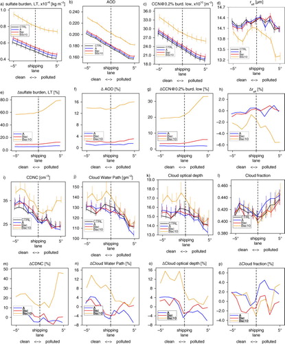
As expected, shipping emissions lead to noticeable across-corridor increases of SU in the lowermost troposphere in all shipping emission scenarios used here (Fig. 2a). However, a distinct change of across-corridor gradient in SU burden at the location of the shipping lane is only apparent in the clearly unrealistic emission scenario employed in simulation Bsc10; the other two simulations merely show an offset w.r.t. CTRL. In relative terms, the increase in SU burden at the shipping lane is also visible for simulations A and Bsc (Fig. 2e). Ultimately, that is, after physical and chemical processing of the shipping emissions in ECHAM5-HAM, the effect on AOD is an increase in all simulations compared to CTRL, giving the impression of a general offset and no distinct change at the location of the imposed shipping lane (Fig. 2b). This also holds for the unrealistic model setup in Bsc10. In relative terms, changes in AOD over the mid-Atlantic Ocean corridor show a slight change in gradient at the location of the imposed shipping lane, whereas the other two simulations show not more than an offset w.r.t. CTRL (Fig. 2f). Changes in AOD FMF, that is, that part of total AOD contributed by particles smaller than 1 µm (not shown), are similar to those for total AOD: a general increase across the whole breadth of the corridor with a slight if any noticeable change at the position of the shipping lane. These findings are similar for the SE Pacific and the mid-Indian Ocean shipping corridors, both of which show lower background values of AOD compared to the mid-Atlantic.

Although across-corridor changes in total AOD only show some indication of shipping-emission influence (Fig. 2b and f), a change in CCN as calculated from Koehler-theory should be expected from the increase in SU loading. As CCN concentrations are unlike AOD independent of ambient relative humidity, they are less influenced by meteorological variability. Indeed, CCN (0.2%) loading in the lower troposphere clearly increases downwind of the imposed shipping lane in model simulations A and Bsc (up to ≈7% for CCN (0.2%)), with this increase being higher in Bsc compared to A (Fig. 2c and g). This is because a much higher number of soluble particles is assigned to a given amount of shipping emissions in Bsc compared to A (cf. P12 for details). In simulations Bsc, the increase is also distinctly more positive in the polluted part compared to A. The ‘offset-like’ structure of across-corridor changes is also apparent. For the unrealistic case of a 10-fold increase in shipping emissions, increases in CCN (0.2%) loading in the lower troposphere are dramatic, with values >30% in the polluted part of the corridor (Fig. 2g).

The non-negligible changes in CCN (0.2%) loading integrated over the lower troposphere hint at a potential effect on water clouds in the shipping corridor of the mid-Atlantic region. However, it turns out that when considering just the across-corridor gradients of absolute values of cloud properties (Fig. 2d, i, j, k and l), it is impossible to distinguish the simulations including shipping emissions from the one not including them. The across-corridor variability (or non-monotonicity) as well as absolute values of cloud property profiles are practically identical for all simulations (except for Bsc10 which shows somewhat of an offset in accordance with AIE hypotheses and shows very large increases in CDNC in the polluted part of the corridor). As expected, CDNC is somewhat anti-correlated with r _eff and the across-corridor profiles of basically correspond to those of LWP. On a side note, this highlights the importance of improving parameterisations of autoconversion in GCMs as current formulations lead to vast overestimations of cloud lifetime effects (effect on e.g. LWP) and therefore overestimate the effect on atmospheric radiation, through the effect on (e.g. Quaas et al., 2009; Wang et al., 2012). The across-corridor profiles of cloud fraction (Fig. 2l and p) also show no statistically significant effect of shipping emissions on cloud properties.

The results of P12 already shed light on these results because they showed that zonally averaged AIEs over tropical areas are slightly negative, but spatial changes in cloud properties over tropical areas are not statistically significant at the 90% level and very similar for all model setups (their Figs. 6 and 12). These negative AIEs thus result from the overall increase in CCN over the whole breadth of the shipping corridors and the poor representation of low-clouds in ECHAM5 (Nam and Quaas, 2012; Nam et al., 2012). Most certainly, this leads to the derived high-variability in P12 and our present study. Therefore, taking into account the uncertainties as given by the error bars in Fig. 2, we confirm that changes in cloud properties over tropical oceans due to shipping emissions are insignificant in ECHAM5-HAM even when rigorous filtering of the model data is applied. Cloud radar observations show that at least regarding the water content of trade wind cumuli, subtle variations in meteorology can more than offset large changes in ambient CCN concentrations (K. Lonitz, personal communication, 2014) – ECHAM5-HAM thus phenomenologically reproduces the observed response of boundary layer clouds to aerosol perturbations.

We also show season-wise composites of the plots shown in Fig. 2 to account for changes in circulation patterns associated with shifts of the ITCZ throughout the year in the Supplementary file. Overall, the findings presented here for 5-yr annual means also hold for the season-wise composites. However, in boreal spring (March–May), the dominating north-easterly winds in the tropical Atlantic lead to an accumulation of ship emitted aerosols and aerosol precursor gases towards the southern edge of the shipping lane. This leads to relative increases of CCN (0.2%) near the surface of more than 20% (the highest of all seasons). However, an effect on cloud properties is not detectable.

Summarising this part of our analysis, we find that cloud and aerosol-population properties respond to shipping emissions over the whole breadth of the shipping corridor rather than showing a distinct change in gradient at the position of the shipping lane itself. Overall, these results are consistent with the findings of P12 who found that despite yielding globally averaged AIEs of up to −0.45±0.02 Wm⁻², AIEs from shipping emissions are not statistically significant anywhere over tropical oceans in ECHAM5-HAM when running it with prescribed SSTs and nudged model dynamics and then averaging the results over a 5-yr period. To this point, it is not entirely clear what causes this broadly spread out change in modelled aerosol- and cloud properties. In the next section, we thus analyse the spatial distribution of aerosol diagnostics obtained from HAM to close in on this issue.

4. Spatially distributed effects of shipping emissions

The results we showed in the previous section leave open the question of how shipping emissions are actually processed in ECHAM5-HAM and why it seems impossible to detect a statistically significant effect of shipping emissions at the location and downwind of main shipping corridors over tropical oceans from satellite remote sensing – despite one of the model simulations yielding an unrealistically high globally averaged AIE of −1.87±0.03 Wm⁻². In this section, we analyse annual mean spatial distributions of model diagnostics characterising the aerosol system to shed light on the processes involved. We use results from model run Bsc, that is, the simulation setup which yields AIEs from shipping emissions of −0.45±0.02 Wm⁻². We also analyse results from simulation Bsc_mAt in which we employ the same emission implementation as Bsc, but with only the emissions of the mid-Atlantic shipping corridor included.

4.1. Global shipping emissions

As in the preceding section, we focus our analysis on the shipping corridor located in the mid-Atlantic Ocean, which contains a zone of substantial shipping emissions outweighing natural emissions of sulphuric species by more than 100% (cf. Fig. 1). For that region, we show maps of 5-yr annual mean ship-emission induced changes of model diagnostics related to aerosol processing in ECHAM5-HAM in Fig. 3. Regarding the emission of aerosols and aerosol precursor gases, we only focus on emissions of sulphuric compounds, comprised of emissions of gaseous SO₂ and primary particulate SU. We do not consider the emissions of BC or OC in detail here because these have been shown nearly irrelevant for determining AIEs from shipping emissions (cf. P12). We remark that the results and conclusions presented here are based on circumstantial evidence from visual analysis. A thorough quantitative evaluation of global aerosol pathways in ECHAM5-HAM is beyond the scope of this study but is a topic of on-going work (N. Schutgens, personal communication, 2013).

Fig. 3 Ship-emission (simulation Bsc) induced 5-yr annual mean absolute and relative changes of sulphur emissions and sinks (a, e and b, f, respectively), sulphate production from gas phase chemistry at 975 and 850 hPa (c, g and d, h, respectively), sulphate production from aqueous oxidation at 975 and 850 hPa (i and j, absolute changes only), total AOD (m, n), CCN concentrations at 0.2% supersaturation at 975 and 850 hPa (k, o and l, p, respectively). Relative changes are derived after . Vectors in (a) indicate the 5-yr mean 10 m wind direction and speed. The black line in (a) shows the assumed location of the windward edge of the shipping lane. The red lines in all panels indicate the part of the shipping lane used to create Fig. 2.

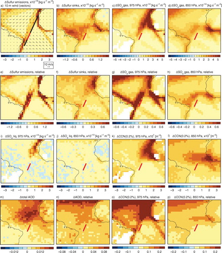
In the mid-Atlantic, the shipping emissions used in the scenario employed in simulation Bsc can locally increase the amount of emitted sulphur by more than 150% at the grid-box scale (Fig. 3e). The across-corridor profiles of sulphur emissions shown in Fig. 1 indicate lower values due to averaging along the shipping lane (black line in Fig. 3a). Dry deposition of SO₂ as calculated by HAM also increases by more than 100% (in terms of sulphur mass, not shown) at the position of the shipping lane, suggesting that much of the emitted sulphur is not available for further chemical and microphysical processing. This possibly contributes to the non-significant changes in aerosol and cloud properties we reported on earlier in this paper (Section 3). We interpret the changes in sulphur sinks (i.e. the sum of dry and wet deposition as well as sedimentation, Fig. 3b and f) and production of SU from gas phase chemistry (Fig. 3c, d, g and h) as evidence that advection of sulphuric species from other shipping corridors in the tropical Atlantic may also hamper the detection of significant AIEs. Especially the shipping emissions located off the coast of Sierra Leone and Liberia (western Africa) result in a more zonal than the expected meridional distribution of aerosol changes at the location of the considered shipping lane (Fig. 3d and h). The relative changes in sulphur sinks and SU production from gas phase chemistry (Fig. 3f, g and h), can also be interpreted as resulting from advection of sulphuric species from the west-African shipping emissions towards the considered shipping lane (black line in Fig. 3a).

The spatial pattern of SU production from liquid phase chemistry (aqueous oxidation), which is generally far more effective than SU production through the gas phase, is spatially limited to the low-level stratocumulus region off the north-west African coast (Fig. 3i and j). This is because i) sulphuric emissions are high just off the African coast, and ii) this region is known to be dominated by low-level clouds, which are captured by the host model (Nam, 2011), thus enabling efficient in-cloud production of SU. In-cloud production of SU leads to a shift of the aerosol size distribution towards larger sizes, which typically increases CCN concentrations (Roelofs et al., 2006). Therefore, aqueous oxidation cannot contribute SU mass to aerosol particles in the main area of interest, which is located further south, possibly limiting the emergence of AIEs. Where non-negligible, we find SU production rates from aqueous oxidation to be roughly one order of magnitude higher than those from gas phase chemistry in the region of interest (compare Fig. 3c, d and i).

Because SU production from aqueous oxidation can only occur in the presence of water clouds, we performed a short analysis of simulated cloud fractions at 975 and 850 hPa in control run CTRL (Supplementary file). At the vertical resolution used here (31 levels), the levels corresponding to 975 and 850 hPa are four model levels apart. Although this simple analysis does not provide information on total vertical cloud extent, it gives a good impression of low-level cloud occurrence in ECHAM5-HAM (see Nam, 2011, for a detailed analysis of cloud vertical distribution in ECHAM5). In the area of interest, 5-yr mean cloud fraction at 975 hPa is on the order of 5–15% just off the northwest African coast, coinciding with the maximum of SU production from aqueous oxidation at that level shown in Fig. 3i. Mean cloud fraction at 975 hPa is smaller than 2% for the rest of the region of interest. At 850 hPa, average cloud fractions are <5% over the entire region of interest. At the same time, the variability of simulated cloud fractions at 975 and 850 hPa in simulation CTRL (in terms of the coefficient of variation, see Supplementary file) is lowest in the region off the northwestern coast of Africa, that is, in the region of the local cloud fraction maximum, and dramatically high over the remaining area of interest. It is now well established that this unrealistic representation of low-cloud variability is not just found in ECHAM5, but in most other current generation GCMs as well (Nam et al., 2012). As this problem is considered the main contributor to uncertainties in cloud-feedback estimates (e.g. Randall et al., 2007; Dufresne and Bony, 2008; Webb et al., 2013), improvements in the representation of low clouds in general circulation models are to be expected in the near future. The simulated small and highly-variable low-level cloud fractions in our simulations then directly translate into small and highly-variable SU production rates from aqueous oxidation. We thus do not show relative changes of SU production from aqueous oxidation in model run Bsc compared to CTRL in Fig. 3 due to very heterogeneous fields showing relative changes in excess of±1000%.

Changes in CCN (0.2%) at 975 hPa are most prominent off the northwest African coast as a result from high SU production rates from aqueous oxidation (Fig. 3k and o) and the associated shift of the aerosol population towards larger sizes (Roelofs et al., 2006). This effect appears pronounced due to the probably overestimated non-convective cloud base updraft velocities [calculated after Lohmann et al., 1999, with modifications presented in Lohmann et al. (2007)] used for deriving the maximum supersaturation (Partanen et al., 2012). This leads to more and smaller particles being activated compared to situations with weaker updrafts. These numerous small particles then contribute to in-cloud SU production, increase in size and therefore increase CCN concentrations (Roelofs et al., 2006). We speculate that weaker updraft velocities would render aqueous oxidation of SU less important for the CCN budget due to fewer smaller particles being considered for activation in the first place. A quantitative assessment of these effects with respect to AIEs from shipping emissions is however beyond the scope of this study.

The mostly zonally oriented pattern of changes in aerosol population at 850 hPa (Fig. 3d and h) leads to almost zonally uniform changes in CCN (0.2%) concentrations at that level (Fig. 3l and p). Considering that the direction of the across-corridor sampling employed in Section 3 is perpendicular to the considered mid-Atlantic shipping lane, and thus almost zonal, it becomes clear why we obtain a substantial increase in CCN concentrations over the whole breadth of the shipping corridor (cf. Fig. 2c and g). The relative increase in CCN (0.2%) concentrations shown in Fig. 2g is much lower than suggested by the increases over much of the region shown in Fig. 3. This is because the data used to create the plots in Fig. 2 does not contain the large relative increases northward of 2N due to sampling constraints. The same applies to the ship-emission induced relative changes in total AOD over the tropical Atlantic as simulated by ECHAM5-HAM (Fig. 3m and n). The substantial absolute increase in AOD off the coast of northern Africa is linked to substantially enhanced SU production through in-cloud aqueous oxidation in the lowermost atmosphere (see above) and the associated particle growth, and is not captured by the sampling of across-corridor aerosol and cloud properties (Fig. 2).

We also show season-wise composites to illustrate the effect of changes in circulation patterns associated with shifts of the ITCZ throughout the year in the Supplementary file. Overall, the findings presented here for 5-yr annual means also hold for the season-wise composites. However, we do find that the effect of tropical deep convection associated with the ITCZ is especially evident in the sulphur sinks: these appear as zonally oriented patches at about 10° latitude during boreal summer and autumn (June–November). In boreal spring (March–May), persistent north-easterly winds lead to an accumulation of ship-emitted aerosol towards the southern edge of the shipping lane. This leads to a substantial relative increase of CCN (0.2%) near the surface at 975 hPa (more than in any other season). Interestingly, these increases in CCN (0.2%) at 975 hPa are mostly associated with negligible changes in AOD, indicating that the common assumption that changes in CCN are proportional to changes in AOD (Andreae, 2009) breaks down on regional scales. Note however that we are comparing CCN changes in the lowermost atmosphere to column integrated AOD.

Although we focus on the mid-Atlantic Ocean shipping corridor here, we also want to shortly comment on our findings regarding the other two corridors investigated in P11, that is, in the south-east (SE) Pacific and the Indian Ocean. As is evident from the across-corridor gradients in sulphur emissions shown in Fig. 1, shipping emissions in the two other corridors represent a far smaller perturbation to the MBL aerosol population than in the one in the mid-Atlantic. In the mid-Indian Ocean (Supplementary file), sulphuric emissions from ships can still locally increase the total emissions of sulphuric species by more than 50%. That large a change in emissions is however confined to grid boxes lying westwards of Mauritius and Reunion, thus not being representative for the analysis due to ‘land contamination’ (see P11). In the region considered for analysis, though, relative increases in sulphuric emissions due to ships are more on the order of 20–30%. Fast removal of sulphuric species very near the point of emission is also evident. Advection of shipping emissions originating to the South of the considered shipping lane plays a minor role here. Changes in CCN (0.2%) concentrations increase by up to 10% directly at the shipping lane; however, this signal is confined to the lowermost atmospheric levels, that is, up to about 850 hPa. Higher altitudes show slight increases in CCN (0.2%) concentrations, these appear however unrelated to the particular shipping corridor. Changes in AOD show an increase in meridional, that is, across-corridor, direction. These are however on the order of 0.01–0.02 and thus within the measurement uncertainty of satellite retrieval algorithms (Remer et al., 2005). In summary, shipping emissions in the mid-Indian Ocean have the potential to slightly elevate CCN (0.2%) concentrations in the MBL. However, as these changes do not appear local, they are diluted and thus remain undetected.

In the SE Pacific Ocean (Supplementary file), we find that the only systematic changes induced by shipping emissions in the simulations with realistic present-day shipping emissions at the considered shipping lane are related to emissions, dry deposition of SO₂ at the shipping lane and production of SU from gas phase chemistry. All other fields show no systematic change with respect to emissions at the shipping lane. Therefore, we conclude that shipping emissions are much too small compared to the natural background emissions in this region for them to have an observationally detectable effect on the local aerosol population and cloud properties.

4.2. Mid-Atlantic shipping emissions only

In the preceding section, we showed that changes in the aerosol population at the shipping corridor located in the mid-Atlantic are partly due to advection of shipping emissions originating upwind of the corridor which have already undergone physical and chemical ageing. Although this explains why we do not find the distinct across-corridor pattern of aerosol changes we expect, it still does not shed light onto the physical processes directly at the shipping lane. In order to isolate the effects of emission processing at the shipping lane from those due to advection, we conducted simulation Bsc_mAt. This sensitivity simulation only includes shipping emissions in the mid-Atlantic Ocean with all else being identical to model setup Bsc. We show spatial distributions of selected aerosol diagnostics in Fig. 4 (similar to Fig. 3).

Fig. 4 As Fig. 3, but for simulation Bsc_mAt.

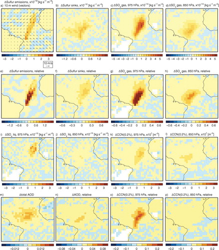
Comparison of the spatial distributions of sulphuric emissions and sinks in Fig. 4a and b confirms the findings from simulation Bsc shown in Fig. 3a and b, namely that much of the emitted aerosols and aerosol precursors are removed from the atmosphere within a few grid-boxes of the shipping corridor. Note that because ECHAM-HAM employs interactive emissions of DMS (Kettle and Andreae, 2000), the differences in sulphur emissions shown in Fig. 4a are not strictly zero anywhere in the domain. The spatial distribution of SU production from gas phase chemistry (Fig. 4c and d) indicates a non-negligible amount of SO₂ being transported downstream away from the shipping corridor, parallel to the northern coast of South America(Fig. 4d and h). Not entirely unrelated, this result supports the sampling strategy laid out in P11, namely that shipping emissions may influence the aerosol population downstream of main shipping corridors. This downstream transport is also evident when analysing the spatial distributions of SU mass mixing ratio and wet deposition fluxes (not shown). As we pointed out earlier, the lack of efficient in-cloud production of SU from aqueous oxidation in the region South of the northern tropical Atlantic stratocumulus fields is probably the main factor limiting aerosol–cloud interactions in the region of interest. If in-cloud SU production near the equator were as large as in the stratocumulus fields further north, that is, about one order of magnitude larger than production from gas phase chemistry despite fewer shipping emissions, the effect on water clouds could be substantial. As a result, we see changes in CCN (0.2%) concentrations at 975 hPa of roughly 10% at the shipping lane (due to efficient production of SU from gas phase chemistry) and changes at 850 hPa are already negligible (<5%) compared to the background concentrations. Since we are interested in comparing the modelled changes in aerosol and cloud properties to the results presented in P11, it is worthwhile noting that the changes in AOD are generally smaller than 0.01 at the shipping lane – a change much too low to be detected reliably by MODIS (Remer et al., 2005).

We do acknowledge that our assessment of the processes at work is still rather speculative at this point. A detailed analysis of aerosol pathways in HAM is beyond the scope of this study, but on-going work gives insights into global aerosol pathways as represented in HAM (N. Schutgens, personal communication, 2013) and the applied method used in that work should prove valuable for future assessments of aerosol processes even on a sector-wise basis.

5. Summary and conclusions

Recent studies employing global modelling and observational efforts suggest a disparity in large scale, climatically relevant AIEs from shipping emissions: modelling suggests substantial effects of up to −0.6 Wm⁻² globally averaged RF (Lauer et al., 2007; Righi et al., 2011; Peters et al., 2012, 2013; Partanen et al., 2013), whereas that obtained from satellite observations is either negligible or undetectable (Devasthale et al., 2006; Schreier et al., 2007; Peters et al., 2011). To bridge the gap between modelling and observational efforts, we applied one of the sampling strategies presented in the observational study of Peters et al. (2011) (P11) to fields obtained from the global modelling effort presented in Peters et al. (2012) (P12) (we used the data from Peters et al. (2013) (P13), though). We complemented the model setup of Peters et al. (2012) by two further simulations. One simulation featured a 10-fold increase in shipping emissions compared to the base case and another additional simulation featured shipping emissions in the mid-Atlantic Ocean only.

The sampling strategy presented in P11 aims at separating areas upwind (‘clean’) and downwind (‘polluted’) of a shipping corridor by sampling for wind direction, the hypothesis being that there exist statistically significant differences in large scale aerosol- and cloud properties between those two areas on climatically relevant scales. Here, we considered the same shipping corridors as in P11 (SE Pacific, mid-Atlantic and mid-Indian Oceans). Additional to the cloud- and aerosol parameters that were studied in the satellite data analysis of P11, we also investigated changes in atmospheric composition, thus eliminating two problems of studies based solely on observations: (1) simulations incorporating shipping emissions (‘sensitivity experiments’) can be compared to a ‘base-case’ and (2) changes in atmospheric composition which may lead to AIEs can also be investigated.

We found increases in aerosol species and boundary layer cloud condensation nuclei (CCN, at 0.2% supersaturation) burdens as well as in AOD across the entire breadth of the shipping corridors in every model realisation. However, the only simulation which shows a distinct relative increase in either one of those properties at the precise location of a shipping lane is the one using a 10-fold increase in shipping emissions representative for the year 2000. In that simulation, we find relative increases in lower tropospheric CCN (0.2%) burdens of more than 30% downwind of the shipping corridor, other model runs yield increases of not more than 5%. Especially the large increase in CCN (0.2%) burdens in the simulation with the 10-fold increased shipping emissions suggested a potentially substantial impact on liquid-cloud micro- and macrophysical properties.

We found that the across-corridor gradients in cloud properties are not significantly different amongst the simulations run with realistic present-day shipping emissions, that is, from visual inspection, it was not possible to determine which one of the realistic model runs was performed with or without prescribing shipping emissions. In other words, even though the simulated globally averaged AIEs from shipping emissions can be very large (up to −0.45 Wm⁻² for the realistic simulations) compared to the current best estimate of total AIEs of −0.45 (−1.2 to 0.0) Wm⁻² (Myhre et al., 2013), detection from space appears limited. We even did not find significantly different cloud properties up- and downwind of shipping lanes when we directly compared these realistic sensitivity experiments to the control simulation. We did however find substantial changes in cloud microphysical properties in the simulation using 10-fold increased shipping emissions.

We also analysed spatial distributions of aerosol diagnostics (sources and sinks of sulphur, production of SU from gas and liquid phase chemistry, CCN concentrations at 0.2% supersaturation and AOD) in the vicinity of shipping lanes over tropical oceans to shed light on the processes leading to undetectable AIEs in these regions. We found that long-range transport of aerosols and aerosol precursor gases emitted upwind of the regions we analysed leads to the changes in aerosol and cloud properties over the entire region. For observational studies of AIEs, this highlights the ever so important and often discussed aspect of correctly defining the background (‘pre-industrial’) reference state against which to gauge the present-day observations. Even in model simulations (which generally only represent nature's complexity to some extent), the effects of uncertainties associated with specifying the reference state show to dominate over those associated with anthropogenic climate forcings (Carslaw et al., 2013).

To isolate changes in aerosol and cloud properties resulting only from local emissions at the shipping lane from those attributable to advection, we masked out all shipping emissions but those corresponding to the major shipping lane in the mid-Atlantic Ocean. We found that shipping emissions indeed lead to changes in the aerosol population downwind of the shipping corridor, thereby supporting the sampling strategy employed in the observational study of P11. However, the resulting changes in CCN (0.2%) were negligible compared to background concentrations. We conjecture that this is due to i) rapid removal of emitted aerosols and aerosol precursor gases from the atmosphere, and ii) inefficient in-cloud production of SU from aqueous oxidation in the considered region. In our simulations, high values of such production rates are confined to the stratocumulus regions off the northwest African coast only. Thus, stratocumulus clouds seem not only more susceptible to anthropogenic emissions of aerosols and aerosol precursors due to their morphology and weak dynamical forcing. Our model simulations also suggest that the presence of the stratocumulus decks themselves elevates CCN concentrations to levels enabling the emergence of AIEs, the underlying process being a shift of the aerosol size distribution towards larger sizes, resulting in more aerosol particles becoming activated as cloud droplets (e.g. Roelofs et al., 2006).

As we focus solely on the influence of shipping emissions on clouds over tropical oceans here, it is worth mentioning that the simulations with ECHAM5-HAM we used here show substantial and statistically significant AIEs over the Northern Hemisphere (NH) parts of the Atlantic and Pacific Oceans (cf. P12). Surely, shipping emissions are much more spread out and substantially larger over those areas. However, the observational detection of AIEs over NH oceans using passive remote sensing is challenging due to the persistent occurrence of multi-layered cloud systems. Case studies such as that of Goren and Rosenfeld (2012) hint at the potential of AIEs from shipping emissions in these NH areas but give little insight into implications at climatically relevant scales. Our analysis however also revealed that over NH oceans, cloud variability in the lower troposphere as simulated by ECHAM5-HAM is far less compared to the tropical regions considered here and therefore allows for a stronger perturbation of the CCN-budget and changes in cloud micro- and macrophysical properties. Partly, this difference in simulated cloud variability exists because ECHAM5, as well as many other current generation GCMs, does a notoriously poor job in representing low clouds over tropical and sub-tropical oceans (Nam et al., 2012). On the other hand, this lack of realism in GCMs makes the effect of aerosol perturbations on oceanic tropical boundary layer clouds appear trumped by cloud dynamics [as found in observations (K. Lonitz, personal communication, 2014)], and thus ‘right for the wrong reason’.

Therefore, the results shown here support the conclusion drawn in P11 that high natural variability of water clouds over tropical oceans is one of the main factors hampering the detection of a signal from satellite data or even limiting the emergence of such a climate forcing (‘dynamics matters more than aerosol’). However, our results also suggest that anthropogenic aerosols may indeed have the potential to influence clouds over tropical oceans other than those located over regions of oceanic upwelling and further research efforts in that direction are warranted. Concerning attempts to quantify climate forcings, such as AIEs, from observations, our results also highlight the importance and non-triviality of adequately determining and accounting for the pre-industrial reference state which one considers as the ‘baseline’ to which observations of present-day climate are gauged.

6. Acknowledgements

We are thankful to four anonymous reviewers for their mostly constructive comments on earlier versions of this paper. We are grateful to Nick Schutgens (University of Oxford, UK) and Katrin Lonitz (MPI-M, Hamburg, Germany) for providing helpful information facilitating the interpretation of our results. The shipping emission inventory was provided in the framework of the European Union FP6 Integrated Project QUANTIFY. The model simulations were performed at the German Computing Centre for Climate and Earth System Research (Deutsches Klimarechenzentrum, DKRZ). K.P. was partly funded by the European Union FP6 Integrated Project QUANTIFY, by the European Commission under the EU Seventh Research Framework Programme (grant 218793, MACC) and by the Australian Research Council within the Centre of Excellence for Climate System Science. P.S.'s research leading to these results has received funding from the European Research Council under the European Union's Seventh Framework Programme (FP7/2007-2013)/ERC grant agreement no. 280025.

Notes

To access the supplementary material to this article, please see Supplementary files under Article Tools online.

References

- Abel S. , Boutle I . An improved representation of the raindrop size distribution for single-moment microphysics schemes. Q. J. Roy. Meterol. Soc. 2012; 138: 2151–2162.
- Andreae M. O . Correlation between cloud condensation nuclei concentration and aerosol optical thickness in remote and polluted regions. Atmos. Chem. Phys. 2009; 9: 543–556.
- Bates T. , Lamb B. , Guenther A. , Dignon J. , Stoiber R . Sulfur emissions to the atmosphere from natural sources. J. Atmos. Chem. 1992; 14: 315–337.
- Behrens H. L . Present traffic and emissions from maritime shipping. Deliverable D1.1.2.2 of the EU-IP QUANTIFY (confidential). 2006. Det Norske Veritas. Online at: http://www.pa.op.dlr.de/quantify/ .
- Bond T. , Streets D. , Yarber K. , Nelson S. , Woo J. , co-authors . A technology-based global inventory of black and organic carbon emissions from combustion. J. Geophys. Res. 2004; 109: D14 203.
- Boucher O. , Randall D. , Artaxo P. , Bretherton C. , Feingold G. , co-authors . Stocker T. , Qin D. , Plattner G.-K. , Tignor M. , Allen S. , co-authors . Clouds and aerosols. Climate Change 2013: The Physical Science Basis. Contribution of Working Group I to the Fifth Assessment Report of the Intergovernmental Panel on Climate Change. 2013; Cambridge, United Kingdom: Cambridge University Press. 571–658.
- Campmany E. , Grainger R. , Dean S. , Sayer A . Automatic detection of ship tracks in ATSR-2 satellite imagery. Atmos. Chem. Phys. 2009; 9: 1899–1905.
- Capaldo K. , Corbett J. , Kasibhatla P. , Fischbeck P. , Pandis S . Effects of ship emissions on sulphur cycling and radiative climate forcing over the ocean. Nature. 1999; 400: 743–746.
- Carslaw K. , Lee L. , Reddington C. , Pringle K. , Rap A. , co-authors . Large contribution of natural aerosols to uncertainty in indirect forcing. Nature. 2013; 503: 67–71.
- Chen Y.-C. , Christensen M. W. , Xue L. , Sorooshian A. , Stephens G. L. , co-authors . Occurrence of lower cloud albedo in ship tracks. Atmos. Chem. Phys. 2012; 12: 8223–8235.
- Christensen M. , Stephens G . Microphysical and macrophysical responses of marine stratocumulus polluted by underlying ships: evidence of cloud deepening. J. Geophys. Res.-Atmos. 2011; 116: D03 201.
- Coakley J. , Bernstein R. , Durkee P . Effect of ship-stack effluents on cloud reflectivity. Science. 1987; 237: 1020–1022.
- Coggon M. M. , Sorooshian A. , Wang Z. , Metcalf A. R. , Frossard A. A. , co-authors . Ship impacts on the marine atmosphere: insights into the contribution of shipping emissions to the properties of marine aerosol and clouds. Atmos. Chem. Phys. 2012; 12: 8439–8458.
- Conover J . Anomalous cloud lines. J. Atmos. Sci. 1966; 23: 778–785.
- Corbett J. , Koehler H . Updated emissions from ocean shipping. J. Geophys. Res. 2003; 108: 4650–64.
- Corbett J. , Koehler H . Considering alternative input parameters in an activity-based ship fuel consumption and emissions model: reply to comment by Øyvind Endresen et al. on Updated emissions from ocean shipping. J. Geophys. Res. 2004; 109: 23303.
- Dalsøren S. , Eide M. , Endresen Ø. , Mjelde A. , Gravir G. , co-authors . Update on emissions and environmental impacts from the international fleet of ships: the contribution from major ship types and ports. Atmos. Chem. Phys. 2009; 9: 2171–2194.
- Dentener F. , Kinne S. , Bond T. , Boucher O. , Cofala J. , co-authors . Emissions of primary aerosol and precursor gases in the years 2000 and 1750 prescribed data-sets for AeroCom. Atmos. Chem. Phys. 2006; 6: 4321–4344.
- Devasthale A. , Krüger O. , Grassl H . Impact of ship emissions on cloud properties over coastal areas. Geophys. Res. Lett. 2006; 33: 02811.
- Dufresne J.-L. , Bony S . An assessment of the primary sources of spread of global warming estimates from coupled atmosphere-ocean models. J. Clim. 2008; 21: 5135–5144.
- Durkee P. , Chartier R. , Brown A. , Trehubenko E. , Rogerson S. , co-authors A . Composite ship track characteristics. J. Atmos. Sci. 2000a; 57: 2542–2553.
- Durkee P. , Noone K. , Bluth R . The Monterey area ship track experiment. J. Atmos. Sci. 2000b; 57: 2523–2541.
- Endresen Ø. , Sørgård E. , Bakke J. , Isaksen I . Substantiation of a lower estimate for the bunker inventory: comment on updated emissions from ocean shipping by James J. Corbett and Horst W. Koehler. J. Geophys. Res. 2004; 109: 23 302.
- Endresen Ø. , Sørgård E. , Sundet J. , Dalsøren S. , Isaksen I. , co-authors . Emission from international sea transportation and environmental impact. J. Geophys. Res. 2003; 108: 4560.
- Eyring V. , Köhler H. , Van Aardenne J. , Lauer A . Emissions from international shipping: 1. The last 50 years. J. Geophys. Res. 2005; 110: 17305.
- Feichter J. , Kjellström E. , Rodhe H. , Dentener F. , Lelieveldi J. , co-authors . Simulation of the tropospheric sulfur cycle in a global climate model. Atmos. Environ. 1996; 30: 1693–1707.
- Franke K. , Eyring V. , Sander R. , Hendricks J. , Lauer A. , co-authors . Toward effective emissions of ships in global models. Meteorol. Z. 2008; 17: 117–129.
- Franklin C. N . A warm rain microphysics parameterization that includes the effect of turbulence. J. Atmos. Sci. 2008; 65: 1795–1816.
- Fuglestvedt J. , Berntsen T. , Eyring V. , Isaksen I. , Lee D. S. , co-authors . Shipping emissions: from cooling to warming of climate – and reducing impacts on health. Environ. Sci. Technol. 2009; 43: 9057–9062.
- Gehlot S. , Quaas J . Convection-climate feedbacks in the ECHAM5 general circulation model: evaluation of cirrus cloud life cycles with ISCCP satellite data from a Lagrangian trajectory perspective. J. Clim. 2012; 25: 5241–5259.
- Goren T. , Rosenfeld D . Satellite observations of ship emission induced transitions from broken to closed cell marine stratocumulus over large areas. J. Geophys. Res. 2012; 117: 17206.
- Grandey B. S. , Stier P. , Wagner T. M . Investigating relationships between aerosol optical depth and cloud fraction using satellite, aerosol reanalysis and general circulation model data. Atmos. Chem. Phys. 2013; 13: 3177–3184.
- Guelle W. , Schulz M. , Balkanski Y. , Dentener F . Influence of the source formulation on modelling the atmospheric global distribution of sea salt aerosol. J. Geophys. Res. 2001; 106: 27509–27524.
- Horowitz L. , Walters S. , Mauzerall D. , Emmons L. , Rasch P. , co-authors . A global simulation of tropospheric ozone and related tracers: description and evaluation of MOZART, version 2. J. Geophys. Res. 2003; 108: 4784.
- Isaksen I. , Granier C. , Myhre G. , Berntsen T. , Dalsren S. , co-authors . Atmospheric composition change: climate chemistry interactions. Atmos. Environ. 2009; 43: 5138–5192.
- Kazil J. , Lovejoy E. R . A semi-analytical method for calculating rates of new sulfate aerosol formation from the gas phase. Atmos. Chem. Phys. 2007; 7: 3447–3459.
- Kazil J. , Stier P. , Zhang K. , Quaas J. , Kinne S. , co-authors . Aerosol nucleation and its role for clouds and earth's radiative forcing in the aerosol-climate model ECHAM5-HAM. Atmos. Chem. Phys. 2010; 10: 10733–10752.
- Kettle A. , Andreae M . Flux of dimethylsulfide from the oceans- a comparison of updated data sets and flux models. J. Geophys. Res. 2000; 105: 793–808.
- Khairoutdinov M. , Kogan Y . A new cloud physics parameterization in a large-eddy simulation model of marine stratocumulus. Mon. Weather Rev. 2000; 128: 229–243.
- Kinne S. , Schulz M. , Textor C. , Guibert S. , Balkanski Y. , co-authors . An AeroCom initial assessment – optical properties in aerosol component modules of global models. Atmos. Chem. Phys. 2006; 6: 1815–1834.
- Kulmala M. , Lehtinen K. E. J. , Laaksonen A . Cluster activation theory as an explanation of the linear dependence between formation rate of 3nm particles and sulphuric acid concentration. Atmos. Chem. Phys. 2006; 6: 787–793.
- Lauer A. , Eyring V. , Hendricks J. , Jöckel P. , Lohmann U . Global model simulations of the impact of ocean-going ships on aerosols, clouds, and the radiation budget. Atmos. Chem. Phys. 2007; 7: 5061–5079.
- Lin H. , Leaitch W . Development of an in-cloud aerosol activation parameterization for climate modelling. Proceedings of the WMO Workshop on Measurement of Cloud Properties for Forecasts of Weather, Air Quality and Climate. 1997; World Meteorological Organization, Geneva 328–335.
- Lin S. , Rood R . Multidimensional flux-form semi-Lagrangian transport schemes. Mon. Weather Rev. 1996; 124: 2046–2070.
- Lohmann U. , Feichter J. , Chuang C. , Penner J . Prediction of the number of cloud droplets in the ECHAM GCM. J. Geophys. Res. 1999; 104: 9169–9198.
- Lohmann U. , Stier P. , Hoose C. , Ferrachat S. , Kloster S. , co-authors . Cloud microphysics and aerosol indirect effects in the global climate model ECHAM5-HAM. Atmos. Chem. Phys. 2007; 7: 3425–3446.
- Lund M. T. , Eyring V. , Fuglestvedt J. , Hendricks J. , Lauer A. , co-authors . Global-mean temperature change from shipping toward 2050: improved representation of the indirect aerosol effect in simple climate models. Environ. Sci. Technol. 2012; 46: 8868–8877.
- Matthias V. , Bewersdorff I. , Aulinger A. , Quante M . The contribution of ship emissions to air pollution in the North Sea regions. Environ. Pollut. 2010; 158: 2241–2250.
- Myhre G. , Shindell D. , Bréon F.-M. , Collins W. , Fuglestvedt J. , co-authors . Stocker T. , Qin D. , Plattner G.-K. , Tignor M. , Allen S. , co-authors . Anthropogenic and natural radiative forcing. Climate Change 2013: The Physical Science Basis. Contribution of Working Group I to the Fifth Assessment Report of the Intergovernmental Panel on Climate Change. 2013; Cambridge, United Kingdom: Cambridge University Press. 659–740.
- Nakajima T. , King M . Determination of the optical-thickness and effective particle radius of clouds from reflected solar-radiation measurements .1 Theory. J. Atmos. Sci. 1990; 47: 1878–1893.
- Nam C. , Bony S. , Dufresne J.-L. , Chepfer H . The ‘too few, too bright’ tropical low-cloud problem in CMIP5 models. Geophys. Res. Lett. 2012; 39: 21 801.
- Nam C. C. W . Using CALIPSO and CloudSat satellite retrievals to evaluate low-level cloud parameterizations in ECHAM5 for cloud-climate feedbacks implications. Berichte zur Erdsystemforschung.
- Nam C. C. W. , Quaas J . Evaluation of clouds and precipitation in the ECHAM5 general circulation model using CALIPSO and CloudSat satellite data. J. Clim.
- Olivier J. G. J. , Van Aardenne J. A. , Dentener F. J. , Pagliari V. , Ganzeveld L. N. , co-authors . Recent trends in global greenhouse gas emissions: regional trends 1970–2000 and spatial distribution of key sources in 2000. Environ. Sci. 2005; 2: 81–99.
- Partanen A.-I. , Kokkola H. , Romakkaniemi S. , Kerminen V.-M. , Lehtinen K. E. J. , co-authors . Direct and indirect effects of sea spray geoengineering and the role of injected particle size. J. Geophys. Res. 2012; 117
- Partanen A. I. , Laakso A. , Schmidt A. , Kokkola H. , Kuokkanen T. , co-authors . Climate and air quality trade-offs in altering ship fuel sulfur content. Atmos. Chem. Phys. 2013; 13: 12059–12071.
- Peters K. , Quaas J. , Graßl H . A search for large-scale effects of ship emissions on clouds and radiation in satellite data. J. Geophys. Res.-Atmos. 2011; 116: 24205.
- Peters K. , Stier P. , Quaas J. , Graßl H . Aerosol indirect effects from shipping emissions: sensitivity studies with the global aerosol-climate model ECHAM-HAM. Atmos. Chem. Phys. 2012; 12: 5985–6007.
- Peters K. , Stier P. , Quaas J. , Graßl H . Corrigendum to “Aerosol indirect effects from shipping emissions: sensitivity studies with the global aerosol-climate model ECHAM-HAM” published in. Atmos. Chem. Phys. 2013; 12: 5985–6007. 2012. Atmos. Chem. Phys. 13, 6429–6430.
- Pierce J. R. , Adams P. J . Uncertainty in global CCN concentrations from uncertain aerosol nucleation and primary emission rates. Atmos. Chem. Phys. 2009; 9: 1339–1356.
- Platnick S. , King M. , Ackerman S. , Menzel W. , Baum B. , co-authors . The MODIS cloud products: algorithms and examples from Terra. IEEE Trans. Geosci. Remote Sens. 2003; 41: 459–473.
- Platnick S. , Twomey S . Determining the susceptibility of cloud albedo to changes in droplet concentration with the Advanced Very High Resolution Radiometer. J. Appl. Meteorol. 1994; 33: 334–347.
- Quaas J. , Ming Y. , Menon S. , Takemura T. , Wang M. , co-authors . Aerosol indirect effects – general circulation model intercomparison and evaluation with satellite data. Atmos. Chem. Phys. 2009; 9: 8697–8717.
- Quaas J. , Stevens B. , Stier P. , Lohmann U . Interpreting the cloud cover – aerosol optical depth relationship found in satellite data using a general circulation model. Atmos. Chem. Phys. 2010; 10: 6129–6135.
- Randall D. , Wood R. , Bony S. , Colman R. , Fichefet T. , co-authors . Solomon S. , Qin D. , Manning M. , Chen Z. , Marquis M. , co-authors . Climate models and their evaluation. Climate Change 2007: The Physical Science Basis. Contribution of Working Group I to the Fourth Assessment Report of the Intergovernmental Panel on Climate Change. 2007; Cambridge, United Kingdom: Cambridge University Press. 589–662.
- Remer L. , Kaufman Y. , Tanre D. , Mattoo S. , Chu D. , co-authors . The MODIS aerosol algorithm, products, and validation. J. Atmos. Sci. 2005; 62: 947–973.
- Righi M. , Klinger C. , Eyring V. , Hendricks J. , Lauer A. , co-authors . Climate impact of biofuels in shipping: global model studies of the aerosol indirect effect. Environ. Sci. Technol. 2011; 45: 3519–3525.
- Roelofs G. J. , Stier P. , Feichter J. , Vignati E. , Wilson J . Aerosol activation and cloud processing in the global aerosol-climate model ECHAM5-HAM. Atmos. Chem. Phys. 2006; 6: 2389–2399.
- Schreier M. , Mannstein H. , Eyring V. , Bovensmann H . Global ship track distribution and radiative forcing from 1 year of AATSR data. Geophys. Res. Lett. 2007; 34: 17814.
- Simmons A. , Uppala S. , Dee D. , Kobayashi S . ERA-Interim: new ECMWF reanalysis products from 1989 onwards. ECMWF Newsletter. 2007; 110: 25–35.
- Stevens B. , Feingold G . Untangling aerosol effects on clouds and precipitation in a buffered system. Nature. 2009; 461: 607–613.
- Stevens R. G. , Pierce J. R . A parameterization of sub-grid particle formation in sulfur-rich plumes for global- and regional-scale models. Atmos. Chem. Phys. 2013; 13: 12117–12133.
- Stevens R. G. , Pierce J. R. , Brock C. A. , Reed M. K. , Crawford J. H. , co-authors . Nucleation and growth of sulfate aerosol in coal-fired power plant plumes: sensitivity to background aerosol and meteorology. Atmos. Chem. Phys. 2012; 12: 189–206.
- Stier P. , Feichter J. , Kinne S. , Kloster S. , Vignati E. , co-authors . The aerosol-climate model ECHAM5-HAM. Atmos. Chem. Phys. 2005; 5: 1125–1156.
- Sundqvist H. , Berge E. , Kristjansson J . Condensation and cloud parameterization studies with a mesoscale numerical weather prediction model. Mon. Weather Rev. 1989; 117: 1641–1657.
- Taylor K. , Williamson D. , Zwiers F . The sea surface temperature and sea-ice concentration boundary conditions for AMIP II simulations. PCMDI Rep. 2000; 60: 28.
- Tegen I. , Harrison S. , Kohfeld K. , Prentice I. , Coe M. , co-authors . Impact of vegetation and preferential source areas on global dust aerosol: results from a model study. J. Geophys. Res. 2002; 107: 4576.
- Tiedtke M . A comprehensive mass flux scheme for cumulus parameterization in large- scale models. Mon. Weather Rev. 1989; 117: 1779–1800.
- Twomey S. , Howell H. , Wojciechowski T . Comments on “anomalous cloud lines.”. J. Atmos. Sci. 1968; 25: 333–334.
- Vignati E. , Wilson J. , Stier P . M7: an efficient size-resolved aerosol microphysics module for large-scale aerosol transport models. J. Geophys. Res. 2004; 109: 22202.
- Wang H. , Feingold G . Modeling mesoscale cellular structures and drizzle in marine stratocumulus. Part II: the microphysics and dynamics of the boundary region between open and closed cells. J. Atmos. Sci. 2009; 66: 3257–3275.
- Wang M. , Ghan S. , Liu X. , L'Ecuyer T. S. , Zhang K. , co-authors . Constraining cloud lifetime effects of aerosols using A-Train satellite observations. Geophys. Res. Lett.
- Wang M. , Ghan S. , Liu X. , L'Ecuyer T. S. , Zhang K. , co-authors . 2012. Constraining cloud lifetime effects of aerosols using A-Train satellite observations. Geophys. Res. Lett.
- Weber T. , Quaas J . Incorporating the subgrid-scale variability of clouds in the autoconversion parameterization using a PDF-scheme. J. Adv. Model. Earth Syst. 2012; 4: 1103.
- Zhang K. , O'Donnell D. , Kazil J. , Stier P. , Kinne S. , co-authors . The global aerosol-climate model ECHAM-HAM, version 2: sensitivity to improvements in process representations. Atmos. Chem. Phys. 2012; 12: 8911–8949.