A model sensitivity study for the sea–air exchange of methane in the Laptev Sea, Arctic Ocean

Abstract

The ocean's sinks and sources determine the concentration of methane in the water column and by that regulating the emission of methane to the atmosphere. In this study, we investigate how sensitive the sea–air exchange of methane is to increasing/decreasing sinks and sources as well as changes of different drivers with a time-dependent biogeochemical budget model for one of the shallow shelf sea in the Siberian Arctic, the Laptev Sea. The applied changes are: increased air temperature, river discharge, wind, atmospheric methane, concentration of nutrients in the river runoff or flux of methane from the sediment. Furthermore, simulations are performed to examine how the large range in observations for methane concentration in the Lena River as well as the rate of oxidation affects the net sea–air exchange. In addition, a simulation with five of these changes applied together was carried out to simulate expected climate change at the end of this century. The result indicates that none of the simulations changed the seawater to becoming a net sink for atmospheric methane and all simulations except three increased the outgassing to the atmosphere. The three exceptions were: doubling the atmospheric methane, decreasing the rivers’ concentration of methane and increasing the oxidation rate where the latter is one of the key mechanisms controlling emission of methane to the atmosphere.

• Arctic Ocean
• Laptev Sea
• methane
• carbon
• sea–air exchange
• modelling

1. Introduction

Methane (CH₄) is an important greenhouse gas that has increased in the atmosphere from around 700 ppb in the mid-eighteenth century to about 1900 ppb at present time (Forster et al., 2007). This increase is attributed to anthropogenic sources such as enteric fermentation, rice agriculture and biomass burning, and the anthropogenic sources account for more than 60% of the total global emission (Judd et al., 2002; IPCC, 2013). However, the largest single natural source of CH₄ to the atmosphere is wetlands. The atmospheric CH₄ has a lifetime of about 8–12 yr (IPCC, 2013) with the major sink being the oxidation of CH₄ to carbon dioxide (CO₂) and water vapour through a reaction sequence initiated by a hydroxyl (OH) radical.

Another natural source of CH₄ to the atmosphere is the ocean. The concentration of CH₄ in the ocean's surface water has been widely observed as supersaturated relative to the atmosphere, the so-called ‘oceanic methane paradox’ [Reeburgh (2007) and references therein], that is, the production of CH₄ in aerobic environment. In addition to this production of CH₄ in the surface water, CH₄ is also produced in the sediment both by microbial and thermogenic methanogenesis. This results in a diffusion of CH₄ from the sediment into the water column where it is affected by horizontally and vertically transport as well as dilution, creating a spatial variability of the CH₄ concentration (Damm et al., 2005). Further, in shallow shelf seas, bubble ebullition from the sea floor to the water column has been observed (Yusupov et al., 2010; Shakhova et al., 2014). The only known process in the water column depleting the concentration of CH₄ is the bacterial oxidation of CH₄ to CO₂, which consequently decreases the flux of CH₄ to the atmosphere.

The supersaturation and a subsurface maximum have been observed in the Laptev Sea (Cramer and Franke, 2005). The Laptev Sea is one of the shallow shelf seas in the Siberian Arctic with an average depth of 48 m and an area of 498 000 km² (Jakobsson, 2002). This sea is highly impacted by the formation and melting of sea-ice as well as from the large amount of freshwater flowing into the sea, mainly from the Lena River. The annual average freshwater discharge from the Lena River is 525 km³ y⁻¹ (Gordeev and Sidorov, 1993) of which about 75–95% occurs during spring break up in late May or beginning of June, owing to the melting of ice and snow in the river and drainage basin. The rivers are an important link between the land and ocean as they transport different constituents, such as CH₄ and nutrients as well as organic matter, recently at an increasing rate as permafrost degrades (Peterson et al., 2002; Frey et al., 2007; Frey and McClelland, 2009; Rawlins et al., 2009).

In this area, the permafrost is mainly continuous both on land and below the seafloor (subsea) (Romanovskii et al., 2005). The subsea permafrost is to a great part continuous to the 50–60 m isobath, with a shift to discontinuous further to the north (Romanovskii et al., 2005). The subsea permafrost was formed during cold periods in the Quaternary when the sea level was low. Holmes and Creager (1974) determined the sea level 50–55 m lower than today about 15 000 yr B.P. with the shoreline close to the shelf edge. This subsea permafrost is proposed to exist down to about 500 m depth (Cramer and Franke, 2005) and may contain a large amount of methane hydrates (Kvenvolden et al., 1993a) as well as organic matter that can decay to CH₄ and CO₂. Methane hydrates are ice-like solids consisting of a lattice of hydrogen-bonded water molecules forming cage-like structures that contain CH₄ gas. If, or when the permafrost thaws, the CH₄ with different origin will probably escape from the seafloor up to the water column through diffusion or bubble ebullition and in this shallow sea, even further into the atmosphere.

The subsea permafrost is more vulnerable to increasing temperature than on-land permafrost because the average annual temperature of the upper 100 m subsea sediment layer is close to thawing. The water temperature close to the sediment is constantly around zero degrees and the sediment is thereby not exposed to the strong freezing in winter that the terrestrial permafrost is. Furthermore, warmer waters of Atlantic origin have been observed to heat the near-bottom Laptev Sea water up to the 20 m isobath (Dmitrenko et al., 2010). These warmer waters have the potential to thaw the subsea permafrost but according to Dmitrenko et al. (2011) this thawing is a process of centuries, but may results in eroding seafloor and release of CH₄ (Shakhova et al., 2010a). In addition to the top-down heating, there is also bottom-up heating where geothermal heat flux thaws the permafrost from beneath and creates open taliks under fault zones. This, together with the top-down heating, can trigger CH₄ release from the sediment.

To investigate how the sea–air exchange is affected by changes in sinks and sources as well as drivers, a time-dependent biogeochemical budget model following Wåhlström et al. (2012), including the carbon system and CH₄, has been applied for the Laptev Sea. Sensitivity tests have been performed to assess how the sea–air exchange of CH₄ responds to different drivers. Further, a combined idealised or ‘worst case scenario’ has been carried out. These analyses are performed to investigate how sensitive the CH₄ sea–air exchange is to changes in the environment, rather than calculating the exact quantitative effect. In this study, we focus on the fate of dissolved CH₄ in the water column. The release of CH₄ from the sediments due to ebullition (Shakhova et al., 2014) is not addressed.

2. Method

2.1. General

A time-dependent biogeochemical budget model was developed for the Laptev Sea (Wåhlström et al., 2012), which in this study has been further extended with a differential equation for CH₄. The model uses the equation solver PROBE (PROgram for Boundary layers in the Environment), a well-documented program for studies of lakes and coastal seas (Omstedt et al., 1994, 2009; Omstedt, 2011; Shaltout and Omstedt, 2012), which is based on 14 differential equations. The generic form of these differential equations is:1

where φ is the dependent variable, t time, z vertical coordinate, W (m s⁻¹) vertical water velocity, Γ _φ (m² s⁻¹) the exchange coefficient and S _φ is the source and sink term for the dependent variable. The first term on the left in eq. (1) is the change in time, the second term vertical advection and the first term to the right represents turbulent diffusion.

The 14 differential equations are divided into six equations for physics and eight for biogeochemistry, including CH₄. The physical part constitutes equations for momentum, heat, salinity and two equations for turbulence (turbulent kinetic energy and its dissipation rate). Except for CH₄, the biogeochemical part consists of equations for dissolved inorganic carbon (DIC), dissolved organic carbon (DOC), total alkalinity (TA), nitrate (NO₃), phosphate (PO₄), oxygen (O₂) and a simplified primary production with one phytoplankton. DIC is defined as the sum of H₂CO₃, HCO₃ ⁻, CO₃ ^{2 −} and CO₂ (aq).

The model covers 50 m depth and has a vertical resolution of 48 layers with the water surface and sediment as the boundary layers. The model used in this study has been improved compared to earlier versions (Wåhlström et al., 2012, 2013) with a parameterisation for the mineralization of phytoplankton in the sediment (M _sed ) according to:2

where A _M is the rate constant (0.1 d⁻¹), B _M is the constant for temperature dependence (0.05°C⁻¹), T the temperature and P the concentration of phytoplankton in the sediment. These constants are adjusted for the model.

The model is forced by meteorological data: air temperature, horizontal wind components (u and v), total cloudiness and relative humidity. These data were provided by NOAA/OAR/ESRL PSD, Boulder, Colorado, USA, and was downloaded for every sixth hour at 77.5°N, 125°E, from the website http://www.esrl.oaa.gov/psd/ (Kalnay et al., 1996).

The model has an estuarine circulation where the inflow of freshwater from the river mixes with incoming high saline deep-water. This mixed surface water flows out of the model domain by geostrophic controlled outflow and Ekman transport, where the latter is dominating and thus the circulation is mainly wind driven, which corresponds with observations (Guay et al., 2001; Dmitrenko et al., 2008). The discharge and properties of freshwater input to the Laptev Sea were taken from the Lena River, the dominating inflow to this sea. The observation data for the Lena River are restricted, and therefore the discharge were calculated as climatological monthly average for the period 1976–1994 from R-ArcticNet, http://www.r-arcticnet.r.nh.du/v3./Points/P6343.html (Lammers et al., 2001). Due to the limited number of observations, it is impossible to take interannual variations into account.

The discharge exhibits a large seasonal variation with small flow between November and May when the river is ice covered. In June, a large peak develops emerging from the melting of ice and snow in the river and drainage basin, which in the model peaks on June 1 each year. After the maximum in June, the discharge decreases almost linearly until it reaches the low winter values in November. The riverine properties considered are heat, salinity, phytoplankton, O₂, NO₃, PO₄, DIC, DOC, TA and CH₄.

2.2. Sensitivity experiments

The sensitivity experiments are compared with a hindcast simulation driven with present day forcings; the latter denoted ‘standard case’ hereafter. The purpose of this study is to assess potential changes in the net sea–air exchange of CH₄ in the Laptev Sea, caused by climate changes (‘indirect’ changes), but also to test various measurements in the Arctic Ocean described in the literature (‘direct’ changes). Finally, a ‘worst case scenario’ simulation is performed. Changes are added directly to the standard case without considering any gradual modification that may occur in reality. Hence, the importance of different drivers rather than the exact quantitative impact is assessed.

In this subsection, the different drivers are outlined. Firstly, the standard case representing present day settings (Section 2.2.1.) and secondly ‘indirect’ changes (Section 2.2.2.) including increased atmospheric temperature or CH₄, increased river discharge, increased riverine nutrient (NO₃ and PO₄) loads or increased wind speed are described. The magnitudes of the changes amount to values projected in climate change scenarios for the end of the 21st century. Third, ‘direct’ changes (Section 2.2.3.) consisting of different observed CH₄ concentration in the Lena River runoff as well as oxidation rate or increased flux from sediment are discussed. These sensitivity experiments are performed to assess how the net sea–air exchange is affected by different estimates of concentrations and fluxes in the literature. Finally, the ‘worst case scenario’ is presented (Section 2.2.4.) where the combined effects of changing drivers are studied (air temperature, wind, river discharge, concentration of CH₄ in the runoff and flux from the sediment).

2.2.1. Standard case

The concentration of CH₄ in the model is affected by oxidation, flux from the sediment, transport with the river discharge, temperature, aerobic production in the subsurface layer and sea–air exchange at the surface. The flux of CH₄ between the surface water and the atmosphere is calculated according to eq. (3) during ice-free conditions. If the sea is ice covered, the flux is reduced to 5% of that calculated by eq. (3), to account for cracks and polynyas (Wåhlström et al., 2013). The sea–air exchange of CH₄, F, is described as a function of the difference between the concentration of CH₄ in the surface water and the air, ΔC, and the transfer velocity for CH₄, k, according to Wanninkhof (1992):3

where4

The coefficient 677 is the Schmidt number for CH₄ at 20°C and salinity 35 (Wanninkhof et al., 2009). W (m s⁻¹) is the wind speed calculated from the horizontal wind components u and v (x and y directions) and Sc (non-dimensional) is the Schmidt number for CH₄ as a function of temperature (Jähne et al., 1987; Wanninkhof, 1992). These are calculated as:5 6

By definition, the sea–air flux of CH₄ from the ocean to the atmosphere is positive, that is, positive and negative values mean outgassing and uptake by the water, respectively (Wanninkhof et al., 2009).

In order to parameterise the subsurface maximum from microbial CH₄ production observed in the Laptev Sea, the formulation for growth of free bacteria from Kantha (2004) was utilised with a rate constant of 0.03 d⁻¹ for the production of CH₄ from the bacteria (Laroche et al., 1999; Lefevre et al., 2002). The constants of the formulation for bacteria growth were adjusted to get a realistic value for the subsurface maximum. The oxidation of CH₄ in the water column follows first-order kinetics (Ward and Kilpatrick, 1990; de Angelis and Scranton, 1993; Kitidis et al., 2010), which is consistent with the formulation in the model. The oxidation rate constant was applied to 4×10⁻⁴ h⁻¹ estimated by Lorenson and Kvenvolden (1995) in the Beaufort Sea, Alaska. Although the constant oxidation rate is a simplification, this approach was applied to investigate how different observed rates affect the sea–air exchange. The concentration of CH₄ in the river water was set to 20 nmol L⁻¹, which is the upper limit from observations of Semiletov et al. (2011), but the value is in the lower part observed by Bussmann (2013). The flux from the sediment was taken from Shakhova et al. (2005) and the atmospheric pCH₄ values were downloaded data from the National Oceanic and atmospheric Administration (NOAA), Point Barrow, Alaska http://www.esrl.noaa.gov/gmd/dv/iadv/graph.php?code=BRW&program=ccgg&type=ts (Dlugokencky et al., 2012).

2.2.2. ‘Indirect’ changes

Increased air temperature: The increased air temperature case represents atmospheric heating due to increased atmospheric partial pressure of CO₂ in climate model scenarios. In this study, we focus on the average result from the B2 emission scenario for this area, with a 4°C temperature increase in the atmosphere (ACIA, 2005) This 4°C rise increases the water temperature, lengthens the ice-free summer season with earlier ice-melt and later sea-ice formation in autumn as well as affects primary productivity (Markus et al., 2009; Wåhlström et al., 2013). The longer ice-free season also gives an elongated period for the sea–air exchange of CH₄ as well as reduced time for CH₄ accumulation under the ice and, consequently, less CH₄ is oxidised to CO₂. It also creates a longer period for the light to penetrate into the surface water, giving an extended growth season for the primary producers (Arrigo et al., 2008). Furthermore, the primary productivity is temperature dependent. Increasing primary production with increasing temperature enhances the subsurface maximum of CH₄ in the model. In addition, the higher water temperature decreases the solubility of CH₄, increasing the outgassing even further.

Increased river discharge: In northern latitudes, a warmer climate amplifies the hydrological cycle (precipitation minus evaporation, snowmelt, etc.) and, as a consequence, the river discharge shows a positive trend (Peterson et al., 2002; Rawlins et al., 2009). Subsequently, the flux of different chemical constituents (e.g. CH₄ and nutrients) to the sea increases with the same percentage. In addition, the halocline gets stronger with the added freshwater in the summer affecting the primary productivity. In this case, an assumption of 25% increase in river discharge is implemented, which is the upper limit of the ACIA (2005) scenarios.

Increased nutrients in river runoff: How the thawing of the permafrost will affect the Siberian rivers’ concentration of nitrate is uncertain (Frey et al., 2007) but the concentration of phosphate is assumed to increase due to mineral weathering in soil waters (Frey and McClelland, 2009). This will probably affect the primary productivity in the Laptev Sea since one of the limiting factors is phosphate (Anderson et al., 2009). To simulate the methane's sensitivity to increasing nutrient loads, a doubling of the concentration of nutrients is applied to the model. This is probably an extreme scenario but gives an idea how the net sea–air exchange of CH₄ reacts to this perturbation in the environment.

Increased wind speed: The cyclonic activity has increased north of Siberia since the mid-1960s (Maslanik et al., 1996; Serreze et al., 2000). However, future projections for the end of the 21st century do not agree in the magnitude of the changes in mean wind speed, direction or extremes (ACIA, 2005). They indicate a possible increase in storm intensity regionally, but also extremes show no consistent changes over the entire Arctic. Hence, in this sensitivity experiment we assume arbitrarily that the wind speed is increased by 10% to illustrate the impact of systematic wind changes on wind-dependent processes such as Ekman driven circulation, ice advection, vertical mixing and the sea–air exchange of gases. This increase by 10% is regarded as an upper limit in future projections.

Increased pCH ₄ in the atmosphere: In this last case for the ‘indirect’ changes, the downloaded atmospheric values for CH₄ are doubled.

2.2.3. ‘Direct’ changes

Changed concentration of CH ₄ in river runoff: The Lena River has the second largest delta in the world, which is located in the continuous permafrost region. Measured CH₄ concentrations in this area vary considerably. For instance, Bussmann (2013) observed CH₄ concentrations of up to 1854 nmol L⁻¹ in 2010 in a creek draining from the permafrost soil into the Lena River. The observed concentrations of CH₄ in the Lena River, delta and estuary vary from 5 up to over 600 nmol L⁻¹ and decrease downstream (Shakhova et al., 2007; Semiletov et al., 2011, 2012; Bussmann, 2013). To examine the effect of observed CH₄ concentration in the river discharge on the sea–air exchange as well as possible increases due to potential permafrost thaw, three cases with different concentrations in the river runoff (5, 60 and 540 nmol L⁻¹) are compared with the 20 nmol L⁻¹ in the standard case.

Increased flux of CH ₄ from sediment: Thawing and degradation of the subsea permafrost are likely to occur but whether the warming is caused by the submergence ~8000 yr B.P. or the recent Arctic climate change is under debate (Petrenko et al., 2010; Shakhova et al., 2010a; Dmitrenko et al., 2011). Observations of ebullition (Yusupov et al., 2010) and elevated bottom concentrations of CH₄ (Shakhova et al., 2010b) have been detected as possible indication of eroding seafloor resulting in increasing release from the sediments. In this study, the ebullition of CH₄ is not considered and only the fluxes of dissolved CH₄ are modelled. In an attempt to estimate the uncertainties caused by the unknown sediment-water fluxes of dissolved CH₄, a twofold increase of the flux of CH₄ from the model's lower boundary is performed.

Changed oxidation rate in the water column: Bacterial oxidation of CH₄ to CO₂ under aerobic conditions is the only known sink for CH₄ in the water column and is therefore an important factor for the sea–air exchange. With a high oxidation rate, the concentration of CH₄ is reduced and the outgassing to the atmosphere decreases and vice versa. In this attempt, two observed oxidation rate constants are compared with the chosen standard case rate constant (4×10⁻⁴ h⁻¹) from Lorenson and Kvenvolden (1995). The higher rate constant is measured by Kitidis et al. (2010) to 3.8×10⁻³ h⁻¹ in the surface water in the Baffin Bay in July 2005. The lower value, 0.02 y⁻¹ (2.3×10⁻⁶ h⁻¹), is observed by Rehder et al. (1999) in the North Atlantic and Labrador Sea in May–June 1997.

2.2.4. ‘Worst case scenario’

The ‘worst case scenario’ simulation combines several of the above-mentioned changes in drivers and is intended to study the combined effect on the Laptev Sea under increased greenhouse gas concentrations in the atmosphere. The ‘worst case scenario’ includes an increase in air temperature with 4°C, 25% increased runoff and 10% increased wind speed. The elevated atmospheric temperature also thaws the permafrost and increases coastal erosion supplying large amount of old soils containing CH₄ into the rivers and shelf seas; therefore, a threefold increase in the river runoff's concentration of CH₄ is applied. Furthermore, the flux from the seafloor is doubled to consider possible seafloor releases. The oxidation rate constant is not changed in this scenario in order to investigate how the boundary affects the concentration of CH₄ in the water column and thereby the sea–air exchange.

3. Results

In this section, the model results for the standard case (Section 3.1.) representing present day settings are presented followed by the results from simulations with ‘indirect’ (Section 3.2.) and ‘direct’ changes (Section 3.3.). Finally, the results from ‘worst case scenario’ are presented (Section 3.4.).

3.1. Standard case

3.1.1. Depth-profile of the CH₄

In Fig. 1, depth-profiles of CH₄ from observations in the Laptev Sea are compared to model output, with (Fig. 1a and c) and without (Fig. 1b and d) in situ production creating a subsurface CH₄ maximum. The observations (Fig. 1a and b) are from an area of 75.20–76.18°N and 121.36–122.17°E, downloaded from the database ‘PANGEA Data Publisher for Earth & Environmental Science’ (Damm et al., 2010). Model outputs are daily averages for July–September 2000–2009 (Fig. 1c and d). The in situ production of CH₄ in the Laptev Sea is unknown, but there are observations indicating that this process is possible in this area (Cramer and Franke, 2005), and therefore we investigate in this study the impact of a potential in situ production (Fig. 1c).

Fig. 1 (a) Observed depth-profile of CH₄ in the Laptev Sea in September 2007 from the PANGEA database, average (red line) and STD (pink area). (b) Observed depth-profile for one profile of CH₄ in the Laptev Sea, September 2007, from the PANGEA database. (c) Modelled daily average of CH₄ (blue line) with in situ production for July–September 2000–2009 and the STD (blue area). (d) The same as (c) but without in situ production. Note the different scales at the x axes.

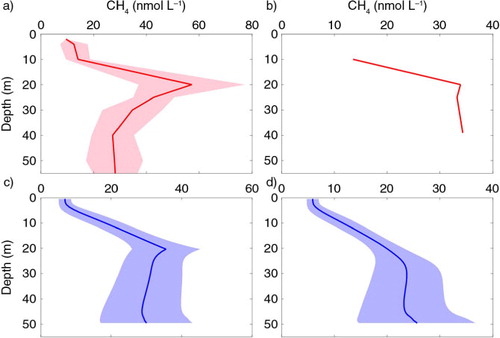
Comparing results of a model simulation with in situ production (Fig. 1c) versus observations (Fig. 1a), we found profiles with similar shape that have lower concentrations at the surface, increasing concentrations with depth down to the subsurface maximum and then decreasing concentrations further to the bottom. Subsurface maxima are present in both observations and model output, although maxima in observations are more pronounced compared to model results. Without the in situ production (Fig. 1b and d), the surface concentration is also low but increases with depth down to 20–25 m. The subsurface maximum is absent with an almost constant concentration below the halocline towards the sea floor where it is slightly increased due to the supply from the sediments.

3.1.2. Surface waters

The model output of surface water temperature, salinity and CH₄ is compared with observations (Fig. 2). The model output for the three constituents is at 4.5 m depth and the temperature and salinity are compared to observed data collected at 4–5 m depth and averaged over an area limited by 115 to 135°E and 74 to 77°N in the Laptev Sea. The observations for the CH₄ values are estimated from the literature between 121–134°E and 69–76°N (Cramer and Franke, 2005; Shakhova et al., 2005, 2009 2010a; Damm et al., 2010).

Fig. 2 Observed (red dots) and modelled surface values (blue solid line) of (a) temperature, (b) salinity, and (c) concentration of CH₄ as function of time and (d) temperature–salinity diagram. Observations for (a), (b) and (d) are horizontal averages over the depth interval 4–5 m in the area between 115 to 135°E and 74 to 77°N. In panel (c), observations are estimated from the literature, see text.

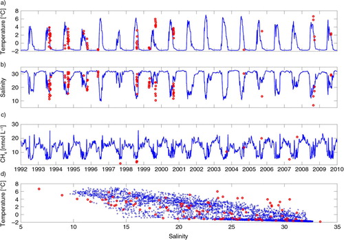
The model captures the annual cycle of the physical and chemical constituents well (Fig. 2). However, the observed variations of temperature are captured better than those of salinity in accordance to Wåhlström et al. (2012). This result is explained by the fact that salinity is much more dependent on the location relative to the freshwater source than temperature. Considering that the model represents an average (horizontal) water column represented by one depth-profile and the observations scarcity and large sampling-area, the model gives a realistic annual cycle with salinities just above 30 during winter and between 10 and 20 during summer.

Observations for CH₄ in the Laptev Sea are very few and even less are available for the research community (Fig. 2c). The model captures the observed variability of CH₄ except for the values during the late 1990s. This can be explained by the concentration of CH₄ in the model's river discharge, which may be too high during the late 1990s affecting the surface water giving the higher value for the model.

3.1.3. Time-series

The model describes a distinct seasonal variability with pronounced summer and winter periods for the surface water (Fig. 3). The stratification starts in late May or beginning of June and depends mostly on the increasing freshwater from the river discharge but also from the melting of sea-ice (Fig. 3a). This freshwater decreases the salinity and establishes a halocline at 10–25 m, which agrees with observations from Bauch et al. (2013), and this halocline hampers the vertical mixing of the water column. In September–October, the salinity increases as a combined effect of decreasing river discharge derived from the freezing of the rivers and their deltas as well as brine release from sea-ice formation that leads to convective mixing. From November to April, the water column is well mixed and the salinity is stable. The thermocline is formed at the same time as the halocline when the sea-ice disappears and the solar radiation starts to warm up the surface waters (Fig. 3b). The maximum surface temperature is in July–August and starts to decrease again, when the atmospheric cooling begins in autumn.

Fig. 3 Modelled time-series for the years 2005–2009: (a) salinity, (b) temperature and (c) concentration of CH₄ as function of depth and time.

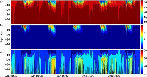
The seasonal signal is also characteristic for the concentration of CH₄ with a well-mixed water column during winter. The surface water is supersaturated relative to the atmosphere from the accumulation of CH₄ under the sea-ice (Kvenvolden et al., 1993b; Semiletov, 1999) hampering the flux of CH₄ to the atmosphere (Fig. 3c). When the ice disappears in late May or beginning of June, the supersaturation in the surface water creates an instant outgassing to the atmosphere, decreasing the concentration in the surface water. The flux of CH₄ proceeds as long as there is open water but the stratification impedes the subsurface surplus to mix up into the surface water and further into the atmosphere. The subsurface maximum of CH₄ in the model is formed at 20 m depth from the bacterial release of CH₄ as the metabolic by-product and the increased concentration mixes into adjacent water masses.

3.1.4. The sea–air exchange of CH₄

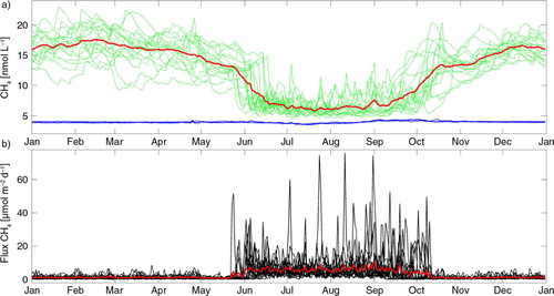
The concentration of CH₄ in the model's surface layer (Fig. 4a) has a seasonal signal and is supersaturated all year round with an average value around 16 nmol L⁻¹ from December to May and with lower, but still supersaturated, values during summer when there is open water and the sea–air exchange occurs (Fig. 4b). In late May or beginning of June, the sea-ice disappears and the concentration of CH₄ decreases rapidly due to outgassing from the supersaturated seawater to the atmosphere (Fig. 4b). In addition, the supersaturated spring flood further enhances the flux to the atmosphere. During summer, the outgassing is an ongoing process (Fig. 4b) with an average CH₄ concentration around 6 nmol L⁻¹ and increasing during autumn until it reaches its winter values in December. In autumn, the brine release from ice production leads to convective mixing, transporting the CH₄ up from deeper water, and the concentration gradient between the deep and surface water disappears. This enhancement creates an increased supersaturation and a way for the deeper CH₄ to be mixed up into the surface water and further into the atmosphere, when the seawater is ice-free.

Fig. 4 (a) Daily mean simulated concentration of CH₄ in the surface layer for the 18-yr (1992–2009) model simulation with present drivers (green line) and the average for the same period (red line). Included are the atmospheric pCH₄ dissolved in seawater for 1992 (blue solid line) and 2009 (blue dotted line) at Point Barrow, Alaska. (b) The corresponding model output of sea–air exchange of CH₄ for the same period (black lines), with the average value shown by the red line. Positive values denote fluxes from the sea to the air.

In Fig. 5, the standard case monthly average net sea–air exchange of CH₄ from May to October for the 18-yr (1992–2009) is compared with the different sensitivity experiments. In May, the net sea–air exchange for the standard case is relatively low but increases in June when the sea-ice disappears and the large spring pulse of river discharge enters the model domain. The outgassing is fairly stable during the summer month, reaching a low value in October when the ice starts to form.

Fig. 5 Modelled monthly average net sea–air exchange for CH₄ from May to October for the 18-yr (1992–2009) model run with different drivers. Standard case is dark blue in both upper and lower panel. Abbreviation to the right stands for: increased air temperature (T^air+4), increased river discharge (Runoff), nutrients in the river (Nuts^river), wind (Wind), CH₄ in the atmosphere [pCH₄(air)], increased concentration of CH₄ in river runoff (CH₄ ^river), flux from the sediment (Flux sed), oxidation rate in the water column (Oxrate) and the ‘worst case scenario’ (scenario). Note the different scales at the y-axes.

The average net sea–air exchange for the 18 yr modelled ice-free period is +6.0 (±1.4) µmol CH₄ m⁻² d⁻¹ (standard deviation in brackets) (Fig. 6 and Table 1), with a maximum of 68 µmol CH₄ m⁻² d⁻¹ (Fig. 4b). Hence, the sea is a source of CH₄ to the atmosphere. Shakhova and Semiletov (2007) calculated area weighted average sea–air exchange for the Laptev Sea and the East Siberian Arctic shelf for 90 d in 2003 to +7.3 µmol CH₄ m⁻² d⁻¹ and in 2004 to +4.5 µmol CH₄ m⁻² d⁻¹. This value is in good agreement with the modelled average net sea–air exchange for the standard case during summer. Taking all the months into account the modelled net average annual flux of CH₄ to the atmosphere, calculated with an area of 498 000 km² (Jakobsson, 2002), is estimated to +0.52 (±0.07) Gmol CH₄ y⁻¹ [+7.29 (±0.98) Gg CH₄ y⁻¹] (Table 1). This result is less than the estimation by Shakhova et al. (2010a), but theirs calculation is for the whole ESAS (the Laptev Sea, East Siberian and the Russian Chukchi Sea) while this study focus on the Laptev Sea only. Rhee et al. (2009) estimated the global oceanic emission to 37–75 Gmol CH₄ y⁻¹ (0.6–1.2 Tg CH₄ y⁻¹) based on observations from the Atlantic Ocean, whereas Bates et al. (1996) calculated it to 25 Gmol CH₄ y⁻¹ from observations in the Pacific Ocean. With respect to these estimates, the Laptev Sea contributes to an annual emission of 0.7–1.4 and 2.1%, respectively, of the global oceanic emission. Considering that, the Laptev Sea constitutes 0.1% of the global oceans area and possible ebullition is not included in this computation, it is a relative high amount of outgassing from this relatively small area.

Fig. 6 Modelled annual average net sea–air exchange (star) and STD (bars) over 18 yr (1992–2009) for the ice-free period for the different experiments. The different simulations are also listed in Table 1 with numbers. Note the two y-axes.

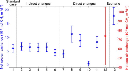
Table 1. Modelled average net seasonal (ice-free period) and annual average net sea–air exchange over 18 yr (1992–2009) for different scenarios

Drivers	No Fig. 6	Average net sea–air CH4 exchange during ice-free period (µmol CH4 m^−2 d^−1)	Average net sea–air CH4 exchange during ice-free period (mg CH4 m^−2 d^−1)	Annual average net sea–air CH4 exchange (Gmol CH4 y^−1)	Annual average net sea–air CH4 exchange (Gg CH4 y^−1)
Standard case	1	+6.0±1.4	+0.08±0.02	+0.52±0.07	+7.29±0.98
‘Indirect’ changes
T^atmosphere+4°C	2	+6.7±1.4	+0.09±0.02	+0.61±0.08	+8.56±1.12
25% increased runoff	3	+6.4±1.5	+0.09±0.02	+0.54±0.08	+7.57±1.12
Nutrients^river * 2	4	+6.3±1.5	+0.09±0.02	+0.54±0.07	+7.57±0.98
10% increased wind speed	5	+6.4±1.6	+0.09±0.02	+0.56±0.07	+7.85±0.98
pCH4 ^atmosphere * 2	6	+4.4±1.1	+0.06±0.02	+0.38±0.05	+5.33±0.70
‘Direct’ changes
CH4 ^river=5 nmol L^−1	7	+4.0±1.5	+0.06±0.02	+0.39±0.07	+5.47±0.98
CH4 ^river=60 nmol L^−1	8	+11.2±3.0	+0.16±0.04	+0.86±0.09	+12.06±1.26
CH4 ^river=540 nmol L^−1	12	+73.9±31.3	+1.04±0.44	+4.92±0.31	+69.01±4.35
Flux from sediment * 2	9	+8.8±2.2	+0.12±0.03	+0.84±0.14	+11.78±1.96
Oxidation rate=3.8×10^−3 h^−1	10	+0.4±0.8	+0.01±0.01	+0.01±0.02	+0.14±0.28
Oxidation rate=2.3×10^−6 h^−1	11	+8.3±2.0	+0.12±0.03	+0.76±0.10	+10.66±1.40
‘Worst case scenario’	13	+17.8±3.1	+0.25±0.04	+1.55±0.17	+21.74±2.38

The results are grouped in scenarios with ‘indirect’ and ‘direct’ changes. The annual average net sea–air exchange is calculated for the Laptev Sea with an area of 498 000 km² (Jakobsson, 2002). The bold numbers in column 3 are statistically significant at the 95% significance level, and blue numbers refer to decreasing values compared with the standard case.

3.2. ‘Indirect’ changes

3.2.1. Increased air temperature with 4°C

The increased temperature results in an enhanced outgassing of CH₄ to the atmosphere. The outgassing is most pronounced in May, September and October compared to the standard case (Fig. 5) when the prolonged ice-free season permits the flux of CH₄ between the atmosphere and the ocean. The average net sea–air exchange for the 120 summer days is +6.7 (±1.4) µmol CH₄ m⁻² d⁻¹ (Fig. 6 and Table 1), an increase with 0.7 (±0.8) µmol CH₄ m⁻² d⁻¹ compared to the standard case. The increase for the 120-d period is statistically significant at the 95% confidence level. Calculated on an annual basis, the net average sea–air exchange is +0.61 (±0.08) Gmol CH₄ y⁻¹ [+8.56 (±1.12) Gg CH₄ y⁻¹], an increase with 0.09 (±0.03) Gmol CH₄ y⁻¹ [+1.27 (±0.14) Gg CH₄ y⁻¹] compared to the standard case (Fig. 6 and Table 1).

3.2.2. Increased river discharge with 25%

The extra nutrient loads enhance the primary productivity increasing the CH₄ concentration in the subsurface maximum. This raise, together with the direct load of extra CH₄ in the runoff, increases the average net sea–air exchange for this case under the 120 summer days (Fig. 6 and Table 1), but the increase is not statistically significant.

3.2.3. Double nutrients in river runoff

Doubling nitrate and phosphate concentrations in the river flow results in almost the same increase in the net sea–air exchange as the increase in the river discharge. Consequently, this case is also not statistically significant (Fig. 6 and Table 1).

3.2.4. Increased wind speed by 10%

An amplified wind speed with 10% does not give a statistically significant change (Fig. 6 and Table 1). It requires a 13% increase to reach a statistically significant change giving a net outgassing of +7.2 (±2.0) µmol CH₄ m⁻² d⁻¹. The net outgassing for this case is higher in all ice-free months (Fig. 5), resulting from both an increase in the sea–air transfer velocity as well as in primary productivity. The increased primary productivity is a result of enhanced wind mixing bringing up nutrients to the surface water promoting the growth of phytoplankton. The net average annual flux for the 13% increase is calculated to +0.64 (±0.07) Gmol CH₄ y⁻¹ [+8.98 (±0.98) Gg CH₄ y⁻¹].

3.2.5. Double pCH₄ in the atmosphere

The amplified concentration of CH₄ in the atmosphere decreases the sea-to-air flux, a result from the reduced gradient between the ocean and the atmosphere. Consequently, the seawater concentration of CH₄ increases. The modelled change in average net sea–air exchange for the summer months is statistically significant, yielding a value of +4.4 (±1.1) µmol CH₄ m⁻² d⁻¹ (Fig. 6 and Table 1), a decrease with 1.6 (±0.3) µmol CH₄ m⁻² d⁻¹ compared to the standard case. As expected, the flux to the atmosphere is lower in all the summer months compared to the standard case, with the largest difference in August as the concentration of CH₄ is at is minimum (Fig. 5). Thus, the annual net average flux in this case is decreasing with 0.14 (±0.02) Gmol CH₄ y⁻¹ [+1.96 (±0.28) Gg CH₄ y⁻¹] to +0.38 (±0.05) Gmol CH₄ y⁻¹ [+5.33 (±0.70) Gg CH₄ y⁻¹] (Table 1). This sensitivity experiment is not adequate since it is not representing real conditions, because all other parameters except the atmospheric CH₄ concentration are kept constant as in the standard case. However, this simulation likely illustrates the integrated effect of the increase in the atmospheric concentration of CH₄ over a longer time and not on a daily basis.

3.3. ‘Direct’ changes

3.3.1. Changed concentration of CH₄ in river runoff

With the concentration of 5, 60 and 540 nmol L⁻¹ in the river runoff, the average net sea–air exchange for the 120 d is +4.0 (±1.5), +11.2 (±3.0) and +73.9 (±31.3) µmol CH₄ m⁻² d⁻¹, respectively. All three changes are statistically significant (Fig. 6 and Table 1). Over the 365 d, this gives a net outgassing to the atmosphere of +0.39 (±0.07), +0.86 (±0.09) and +4.92 (±0.31) Gmol CH₄ y⁻¹ [+5.47 (±0.98), +12.06 (±1.26), +69.01 (±4.35) Gg CH₄ y⁻¹], respectively. The largest deviation in the flux compared with the standard case is in June when the large spring flood enters the sea (Fig. 5). The spring flood in June emerges from the melting of ice and snow in the river and drainage basin. The river melts from south towards north and, consequently, the sea level rises as the melting propagates northwards and a strong pulse of freshwater enters the sea when the northernmost ice melts, creating a strong stratification in the sea. After the maximum in June, the runoff decreases almost linearly until it reaches its winter values. This is reflected in the outgassing for the 60 and 540 nmol L⁻¹ cases. The outgassing increases drastically in June due to the spring flood and then decreases as the discharge declined (Fig. 5), which may be an indication for the river runoff's importance on the net sea–air exchange. The 5 nmol L⁻¹ case creates reduced outgassing compared with the standard case, with highest value in August but still lower than the standard case, which is caused by the decreasing gradient between the seawater and the ocean.

3.3.2. Increased flux of CH₄ from sediment

The higher concentration supplied from the sediment is mixed up into the water column enhancing the concentration of CH₄ all the way up to the surface. This surplus of CH₄ creates a higher flux into the atmosphere in all summer months compared to the standard case (Fig. 5). In wintertime, the water column is well mixed and the CH₄ from the deep-water accumulates under the sea-ice creating a strong outgassing to the atmosphere during the ice break up in spring. The result of the modelled average net sea–air exchange for the 120 summer days is +8.8 (±2.2) µmol CH₄ m⁻² d⁻¹ (Fig. 6 and Table 1), a statistically significant increase with 2.8 (±0.9) µmol CH₄ m⁻² d⁻¹ compared to the standard case. The annual average outgassing is calculated to +0.84 (±0.14) Gmol CH₄ y⁻¹ [+11.78 (±1.96) Gg CH₄ y⁻¹], an increase by 0.33 (±0.07) Gmol CH₄ y⁻¹ [+4.49 (±0.98) Gg CH₄ y⁻¹] compared to the standard case.

3.3.3. Changed oxidation rate in the water column

Utilising the smallest chosen, first-order rate constant (2.3×10⁻⁶ h⁻¹) increases the CH₄ in the water column and, as a consequence, the net sea-to-air exchange increases with 2.3 (±0.8) µmol CH₄ m⁻² d⁻¹ to +8.3 (±2.0) µmol CH₄ m⁻² d⁻¹ compared to the standard case, a statistically significant increase. This gives an annual average value of +0.76 (±0.10) Gmol CH₄ y⁻¹ [+10.66 (±1.40) Gg CH₄ y⁻¹], an increase by 0.24 (±0.04) Gmol CH₄ y⁻¹ [+3.37 (±0.42) Gg CH₄ y⁻¹] compared to the standard case.

For the largest chosen, first-order rate constant (3.8×10⁻³ h⁻¹), the average concentration of CH₄ for the modelled 18 yr is undersaturated during the whole year except for June–July when the large spring flood flushes into the model creating supersaturated water. However, the net sea-to-air exchange is still positive with a value of +0.4 (±0.8) µmol CH₄ m⁻² d⁻¹, a statistically significant reduction with 5.6 (±1.6) µmol CH₄ m⁻² d⁻¹. The annual average net outgassing for this case is +0.01 (±0.02) µmol CH₄ y⁻¹ [+0.14 (±0.28) Gg CH₄ y⁻¹], a decrease with 0.51 (±0.07) Gmol CH₄ y⁻¹ [+7.15 (±0.70) Gg CH₄ y⁻¹].

3.4. ‘Worst case scenario’

The result for the combined future scenario simulation is statistically significant with a net sea–air exchange of +17.8 (±3.1) µmol CH₄ m⁻² d⁻¹, an increase with 11.8 (±2.4) µmol CH₄ m⁻² d⁻¹ compared with the standard case (Fig. 6 and Table 1). The highest percentage increase is calculated in May and October, originating partly from the earlier sea-ice melt, which is a consequence of the increasing air temperature, partly from the well-mixed water column transporting the surplus of CH₄ from the sediment up into the surface layer. In addition, the increased wind speed contributes to this increase as it enhances the transfer velocity (Fig. 5). However, the daily outgassing is highest in June when the large spring flood flushes into the model domain affecting both the concentration of CH₄ but also triggers the primary productivity increasing the subsurface maximum, which mixes up into to surface water. After this maximum in June, the net sea–air exchange decreases slowly to its winter value. The annually net average outgassing for the ‘worst case scenario’ increases with 1.03 (±0.10) Gmol CH₄ y⁻¹ [+14.45 (±1.40) Gg CH₄ y⁻¹] to +1.55 (±0.17) Gmol CH₄ y⁻¹ [+21.74 (±2.38) Gg CH₄ y⁻¹].

4. Discussion

The results show that the considered ‘direct’ changes have a larger impact on the net sea–air exchange of CH₄ in the Laptev Sea than the ‘indirect’ changes even if the latter changes in the atmosphere (increased temperature and CH₄) are statistical significant at the 95% confidence level and increase/decrease the outgassing from the ocean to the atmosphere. All three ‘direct’ changes (the oxidation rate, the concentration of CH₄ in the river runoff and the CH₄ flux from the sediment) are statistically significant.

With increasing air temperature, the season with open water is extended and consequently a prolonged growth season for the primary producers as well as an elongated period for the sea–air exchange of CH₄ occurs (Arrigo et al., 2008; Markus et al., 2009), increasing the net flux to the atmosphere. Furthermore, with earlier sea-ice retreat an even further increased CH₄ flux to the atmosphere is expected as the accumulation of CH₄ under the ice is limited and the time for oxidation to CO₂ is reduced, creating a positive feedback to a warming climate. The simulations reveal the importance of the oxidation rate constant and crucial necessity to do in situ measurement of the oxidation rate constant, not least for the modelling community to catch the right concentration of CH₄ in the water column. The oxidation rate constant has a large impact on how much CH₄ is oxidised to CO₂ and, consequently, how much CH₄ outgasses to the atmosphere.

Another unresolved factor for CH₄ is how the incoming river runoff's concentration of CH₄ affects the budget and net sea–air exchange of CH₄ in the Laptev Sea. The observed concentrations of CH₄ in the Lena River, delta and estuary vary considerably in magnitude and are observed to decrease from the river towards the open sea, probably due to outgassing from the supersaturated river water to the atmosphere (Shakhova et al., 2007; Semiletov et al., 2011, 2012; Bussmann, 2013). Hence, the role of riverine CH₄ loads for the CH₄ concentration in the Laptev Sea is unsolved, in particular if the permafrost in the catchment area of the Lena River thaws and large amounts of carbon reach the coastal zone. To estimate the uncertainties of our study, the concentration of CH₄ in the river runoff was increased by a factor three or 27 as well as decreased by a factor four in an attempt to simulate how river loads influence the net sea–air exchange of CH₄. If CH₄ in the inflowing river water decreases from 20 to 5 nmol L⁻¹, the flux to the atmosphere will be reduced by 33% during the ice-free season. However, if concentrations in the river are elevated to 60 or 540 nmol L⁻¹, the net sea–air fluxes will increase by 87 or 1130%, respectively. In this sensitivity study, the latter is the largest increase for the outgassing to the atmosphere. These changes in concentration may provide an indication for the rivers’ role for the CH₄ budget and for the net sea–air exchange.

The third uncertainty factor is the supply of CH₄ from the sediment. Since the mid-1980s, a warming of 2.1° in summer has been recorded in the bottom water of the Laptev Sea inner shelf with depths in the range of 0–10 m (Dmitrenko et al., 2011). It is not clear whether it is this recent increase in temperature or if it is the warming initiated by submerging ˜8000 yr B.P. that cause the observed ebullition (Shakhova et al., 2014) and elevated bottom concentration of CH₄. This topic is out of the scope of the present study. Here, we focus on the slower diffusion of dissolved CH₄ released from the sediment and its impact on the net sea–air exchange. The bubble plume from the sediment originating from degrading permafrost is not considered in this study. We assume that in case of ebullition a substantial amount of the bubble flux from the shallow sea bottom reaches the atmosphere unaffected within a short time. This latter assumption depends on the specific features of the bubbles as well as on environmental conditions (Judd et al., 1997; Leifer and Patro, 2002). To test the sensitivity on the net sea–air exchange, the flux from the sediment into the bottom layer is doubled. We found that the concentration of CH₄ in the whole water column increases due to vertical mixing. Consequently, the flux to the atmosphere during the ice-free season increases by 47%.

Cramer and Franke (2005) observed a subsurface maximum of CH₄ in the Laptev Sea generated from microbial production in 1997, which to our knowledge is the only published study of δ¹³C_CH4 in the water column for this area determining the CH₄ sources. These observations indicate the possibility of bacterial in situ production of CH₄ in this area. However, the in situ produced CH₄ has a lower concentration than the CH₄ supplied from the sediment and is therefore often overshadowed by the higher concentration from the sediment. In situ CH₄ production was suggested by Karl and Tilbrook (1994) where methanogens within particulate biogenic materials produce CH₄. This production occurs in the depth of the pycnocline where the organic material sinks and accumulates. Furthermore, aerobic in situ production of CH₄ is proposed as the metabolic by-product from bacteria utilising methylphosphonate (MPn) or dimethylsulfoniopropionate (DMSP) as a phosphate or carbon source, respectively (Karl et al., 2008; Damm et al., 2010; Metcalf et al., 2012; Kamat et al., 2013). The in situ CH₄ production in the surface water was also described by Damm et al. (2008) from observations in Storfjorden in the Svalbard Archipelago. In this study, we investigate the impact of the hypothetical in situ CH₄ production with the help of an additional experiment where the bacterial production was removed from the standard case (Fig. 1d). The results show that the bacterial production in the standard case accounts for 36 and 27% of the net air–sea exchange for the ice-free and annual periods, respectively.

For the ‘indirect’ changes, we found statistically significant changes in the net sea–air exchange for the 4°C rise in air temperature and for the twofold pCH₄ in the atmosphere. The other three experiments (increased river discharge, increased riverine nutrient loads and increased wind speed) did not result in statistically significant changes. However, the wind speed is important for the sea–air exchange (Shakhova et al., 2014), especially for ebullition. According to our model results, an increase in wind speed by 13% is required to obtain a significant increase at the 95% confidence level for the net sea–air exchange. This increase would be accomplished after about 30 yr assuming a trend in wind speed as estimated by Spreen et al. (2011) for the Arctic Basin during the period 2000–2009. For this trend analysis, Spreen et al. (2011) used four different reanalysis datasets.

A simulation for a ‘worst case’ future scenario resulted in an increased outgassing to the atmosphere by almost three times for the 120 ice-free days. Overall, the different changes in this simulation contribute to an increased outgassing to the atmosphere due to the increased water column's concentration of CH₄. The largest single contribution to this increase is the threefold increase in the river concentration of CH₄. However, the annual average outgassing would have been 27% higher if the oxidation of CH₄ to CO₂ had not acted as a sink on the CH₄ concentration.

This is, to our knowledge, the first attempt to investigate how the net sea–air exchange of CH₄ is affected by environmental changes or by different parameterisations of processes. In the future, in situ measurements and model improvement will provide us with even further understanding on how the different sources and sinks as well as internal feedbacks influence the flux of CH₄ to the atmosphere. One important modification in the model is to incorporate an oxidation rate constant that depends on temperature and added supply, both from the river runoff and sediment.

5. Conclusions

The Laptev Sea is one of the shallow shelf seas in the Siberian Arctic, which act as a source of CH₄ to the atmosphere. By utilising a time-dependent biogeochemical budget model, the sensitivity of the net sea–air exchange of CH₄ forced by different drivers is studied as well as a future scenario. A validation show that the model reproduces realistic value of the CH₄ concentrations in the water column, the sources and sinks as well as the sea–air exchange of CH₄ in the Laptev Sea. The results indicate that the rivers’ concentration of CH₄ and the supply from the sediment affect the sea–air exchange of CH₄ and can be important factors for this process as well as the oxidation of CH₄ to CO₂ in the water column. However, the estimations of CH₄ in the literature contain large uncertainties, especially for the oxidation rate constant, which points to the importance of additional in situ measurements of these processes. The ‘worst case’ future scenario simulation revealed an increasing outgassing of CH₄ to the atmosphere by almost three times compared to present forcing. This increase was mainly due to increasing CH₄ concentration in the river runoff.

6. Acknowledgements

Funding from the Nordic Council of Ministers within the Top-level Research Initiative (TRI) program ‘Biogeochemistry in a changing cryosphere – depicting ecosystem-climate feedbacks as affected by changes in permafrost, snow and ice distribution’ (DEFROST); from the Swedish Research Council for Environment, Agricultural Sciences and Spatial Planning (FORMAS) within the strategic research area ‘Advanced Simulation of Arctic climate change and impact on Northern regions’ (ADSIMNOR, reference 214-2009-389); and from Stockholm University's Strategic Marine Environmental Research Funds ‘Baltic Ecosystem Adaptive Management (BEAM)’ is gratefully acknowledged. We thank two anonymous reviewers for their helpful suggestions to improve the manuscript.

References

- ACIA. Arctic Climate Impact Assessment.
- Anderson L. G. , Jutterstrom S. , Hjalmarsson S. , Wahlstrom I. , Semiletov I. P . Out-gassing of CO2 from Siberian Shelf seas by terrestrial organic matter decomposition. Geophys. Res. Lett. 2009; 36: 6–9.
- Arrigo K. R. , van Dijken G. , Pabi S . Impact of a shrinking Arctic ice cover on marine primary production. Geophys. Res. Lett. 2008; 35: L19603.
- Bates T. S. , Kelly K. C. , Johnson J. E. , Gammon R. H . A reevaluation of the open ocean source of methane to the atmosphere. J. Geophys. Res. Atmos. 1996; 101: 6953–6961.
- Bauch D. , Torres-Valdes S. , Polyakov I. , Novikhin A. , Dmitrenko I. , co-authors . Halocline water modification and along slope advection at the Laptev Sea continental margin. Ocean Sci. 2013; 10: 1581–1617.
- Bussmann I . Distribution of methane in the Lena Delta and Buor-Khaya Bay, Russia. Biogeosciences. 2013; 10: 4641–4652.
- Cramer B. , Franke D . Indications for an active petroleum system in the Laptev Sea, NE Siberia. J. Petrol. Geol. 2005; 28: 369–383.
- Damm E. , Helmke E. , Thoms S. , Schauer U. , Nothig E. , co-authors . Methane production in aerobic oligotrophic surface water in the central Arctic Ocean. Biogeosciences. 2010; 7: 1099–1108.
- Damm E. , Kiene R. P. , Schwarz J. , Falck E. , Dieckmann G . Methane cycling in Arctic shelf water and its relationship with phytoplankton biomass and DMSP. Mar. Chem. 2008; 109: 45–59.
- Damm E. , Mackensen A. , Budeus G. , Faber E. , Hanfland C . Pathways of methane in seawater: plume spreading in an Arctic shelf environment (SW-Spitsbergen). Continent. Shelf. Res. 2005; 25: 1453–1472.
- de Angelis M. A. , Scranton M. I . Fate of methane in the Hudson river and estuary. Global. Biogeochem. Cycles. 1993; 7: 509–523.
- Dlugokencky E. J. , Lang P. M. , Crotwell A. M. , Masarie K. A . Atmospheric Methane Dry Air Mole Fractions from the NOAA ESRL Carbon Cycle Cooperative Global Air Sampling Network, 1983–2011. 2012. Version: 2012-09-24, ESRL Carbon Cycle, Boulder, CO.
- Dmitrenko I. A. , Kirillov S. A. , Tremblay L. B . The long-term and interannual variability of summer fresh water storage over the eastern Siberian shelf: implication for climatic change. J. Geophys. Res. Oceans. 2008; 113: C03007.
- Dmitrenko I. A. , Kirillov S. A. , Tremblay L. B. , Bauch D. , Holemann J. A. , co-authors . Impact of the Arctic Ocean Atlantic water layer on Siberian shelf hydrography. J. Geophys. Res. Oceans. 2010; 115: 17.
- Dmitrenko I. A. , Kirillov S. A. , Tremblay L. B. , Kassens H. , Anisimov O. A. , co-authors . Recent changes in shelf hydrography in the Siberian Arctic: potential for subsea permafrost instability. J. Geophys. Res. Oceans. 2011; 116: C10027.
- Forster P. , Ramaswamy V. , Artaxo P. , Berntsen T. , Betts R. , co-authors . Solomon S. , Qin D. , Manning M. , Chen Z. , Marquis M. , co-authors . Changes in atmospheric constituents and in radiative forcing. Climate Change 2007: The Physical Science Basis. 2007; Cambridge, United Kingdom: Cambridge University Press. 129–234. Contribution of Working Group I to the Fourth Assessment Report of the Intergovernmental Panel on Climate Change.
- Frey K. E. , McClelland J. W . Impacts of permafrost degradation on arctic river biogeochemistry. Hydrolog. Process. 2009; 23: 169–182.
- Frey K. E. , McClelland J. W. , Holmes R. M. , Smith L. C . Impacts of climate warming and permafrost thaw on the riverine transport of nitrogen and phosphorus to the Kara Sea. J. Geophys. Res. Oceans. Biogeosciences. 2007; 112: 10.
- Gordeev V. V. , Sidorov I. S . Concentrations of major elements and their outflow into the Laptev Sea by the Lena River. Mar. Chem. 1993; 43: 33–45.
- Guay C. K. H. , Falkner K. K. , Muench R. D. , Mensch M. , Frank M. , co-authors . Wind-driven transport pathways for Eurasian Arctic river discharge. J. Geophys. Res. Oceans. 2001; 106: 11469–11480.
- Holmes M. L. , Creager J. S . Herman Y . Holocene history of the Laptev Sea continental shelf. Marine Geology and Oceanography of the Arctic Seas. 1974; New York: Springer-Verlag. 211–229.
- IPCC. Stocker T. F. , Qin D. , Plattner G.-K. , Tignor M. , Allen S. K. , co-authors . Climate change 2013: the physical science basis. Contribution of Working Group I to the Fifth Assessment Report of the Intergovernmental Panel on Climate Change.
- Jakobsson M . Hypsometry and volume of the Arctic Ocean and its constituent seas. Geochem. Geophys. Geosys. 2002; 3
- Judd A. , Davies G. , Wilson J. , Holmes R. , Baron G. , co-authors . Contributions to atmospheric methane by natural seepages on the UK continental shelf. Mar. Geol. 1997; 138: 165–189.
- Judd A. G. , Hovland M. , Dimitrov L. I. , Garcia-Gil S. , Jukes V . The geological methane budget at Continental Margins and its influence on climate change. Geofluids. 2002; 2: 109–126.
- Kalnay E. , Kanamitsu M. , Kistler R. , Collins W. , Deaven D. , co-authors . The NCEP/NCAR 40-year reanalysis project. Bull. Am. Meteorol. Soc. 1996; 77: 437–471.
- Kamat S. S. , Williams H. J. , Dangott L. J. , Chakrabarti M. , Raushel F. M . The catalytic mechanism for aerobic formation of methane by bacteria. Nature. 2013; 497: 132–136.
- Kantha L. H . A general ecosystem model for applications to primary productivity and carbon cycle studies in the global oceans. Ocean Model. 2004; 6: 285–334.
- Karl D. M. , Beversdorf L. , Bjorkman K. M. , Church M. J. , Martinez A. , co-authors . Aerobic production of methane in the sea. Nat. Geosci. 2008; 1: 473–478.
- Karl D. M. , Tilbrook B. D . Production and transport of methane in oceanic particulate organic-matter. Nature. 1994; 368: 732–734.
- Kitidis V. , Upstill-Goddard R. C. , Anderson L. G . Methane and nitrous oxide in surface water along the North-West Passage, Arctic Ocean. Mar. Chem. 2010; 121: 80–86.
- Kvenvolden K. A. , Ginsburg G. D. , Soloviev V. A . Worldwide distribution of subaquatic gas hydrates. Geo Mar. Lett. 1993a; 13: 32–40.
- Kvenvolden K. A. , Lilley M. D. , Lorenson T. D. , Barnes P. W. , Mclaughlin E . The Beaufort Sea Continental-Shelf as a seasonal source of atmospheric methane. Geophys. Res. Lett. 1993b; 20: 2459–2462.
- Lammers R. B. , Shiklomanov A. I. , Vorosmarty C. J. , Fekete B. M. , Peterson B. J . Assessment of contemporary Arctic river runoff based on observational discharge records. J. Geophys. Res. Atmos. 2001; 106: 3321–3334.
- Laroche D. , Vezina A. F. , Levasseur M. , Gosselin M. , Stefels J. , co-authors . DMSP synthesis and exudation in phytoplankton: a modeling approach. Mar. Ecol. Prog. Ser. 1999; 180: 37–49.
- Lefevre M. , Vezina A. , Levasseur M. , Dacey J. W. H . A model of dimethyl sulfide dynamics for the subtropical North Atlantic. Deep. Sea. Res. Oceanogr. Res. Paper. 2002; 49: 2221–2239.
- Leifer I. , Patro R. K . The bubble mechanism for methane transport from the shallow sea bed to the surface: a review and sensitivity study. Continent. Shelf. Res. 2002; 22: 2409–2428.
- Lorenson T. D. , Kvenvolden K. A . Methane in Coastal Water, Sea Ice, and Bottom Sediments, Beaufort Sea, Alaska. 1995. Open-File Report 95–70, U.S. Department of the Interior, U.S. Geological Survey, Menlo Park, California.
- Markus T. , Stroeve J. C. , Miller J . Recent changes in Arctic sea ice melt onset, freeze up, and melt season length. J. Geophys. Res. Oceans. 2009; 114: C12024.
- Maslanik J. A. , Serreze M. C. , Barry R. G . Recent decreases in Arctic summer ice cover and linkages to atmospheric circulation anomalies. Geophys. Res. Lett. 1996; 23: 1677–1680.
- Metcalf W. W. , Griffin B. M. , Cicchillo R. M. , Gao J. T. , Janga S. C. , co-authors . Synthesis of methylphosphonic acid by marine microbes: a source for methane in the Aerobic Ocean. Science. 2012; 337: 1104–1107.
- Omstedt A . Guide to Process Based Modelling of Lakes and Coastal Seas. 2011; Springer-Praxis books in Geophysical Sciences, Springer-Verlag Berlin, Heidelberg.
- Omstedt A. , Carmack E. C. , Macdonald R. W . Modeling the seasonal cycle of salinity in the MacKenzie shelf estuary. J. Geophys. Res. Oceans. 1994; 99: 10011–10021.
- Omstedt A. , Gustafsson E. , Wesslander K . Modelling the uptake and release of carbon dioxide in the Baltic Sea surface water. Continent. Shelf. Res. 2009; 29: 870–885.
- Peterson B. J. , Holmes R. M. , McClelland J. W. , Vorosmarty C. J. , Lammers R. B. , co-authors . Increasing river discharge to the Arctic Ocean. Science. 2002; 298: 2171–2173.
- Petrenko V. V. , Etheridge D. M. , Weiss R. F. , Brook E. J. , Schaefer H. , co-authors . Methane from the East Siberian Arctic Shelf. Science. 2010; 329: 1146–1147.
- Rawlins M. A. , Serreze M. C. , Schroeder R. , Zhang X. D. , McDonald K. C . Diagnosis of the record discharge of Arctic-draining Eurasian rivers in 2007. Environ. Res. Lett. 2009; 4: 045011.
- Reeburgh W. S . Oceanic methane biogeochemistry. Chem. Rev. 2007; 107: 486–513.
- Rehder G. , Keir R. S. , Suess E. , Rhein M . Methane in the northern Atlantic controlled by microbial oxidation and atmospheric history. Geophys. Res. Lett. 1999; 26: 587–590.
- Rhee T. S. , Kettle A. J. , Andreae M. O . Methane and nitrous oxide emissions from the ocean: a reassessment using basin-wide observations in the Atlantic. J. Geophys. Res. Atmos. 2009; 114: D12304.
- Romanovskii N. N. , Hubberten H. W. , Gavrilov A. V. , Eliseeva A. A. , Tipenko G. S . Offshore permafrost and gas hydrate stability zone on the shelf of East Siberian Seas. Geo-Mar. Lett. 2005; 25: 167–182.
- Semiletov I. P . Aquatic sources and sinks of CO(2) and CH(4) in the polar regions. J. Atmos. Sci. 1999; 56: 286–306.
- Semiletov I. P. , Pipko I. I. , Shakhova N. E. , Dudarev O. V. , Pugach S. P. , co-authors . Carbon transport by the Lena River from its headwaters to the Arctic Ocean, with emphasis on fluvial input of terrestrial particulate organic carbon vs. carbon transport by coastal erosion. Biogeosciences. 2011; 8: 2407–2426.
- Semiletov I. P. , Shakhova N. E. , Sergienko V. I. , Pipko I. I. , Dudarev O. V . On carbon transport and fate in the East Siberian Arctic land-shelf-atmosphere system. Environ. Res. Lett. 2012; 7: 015201.
- Serreze M. C. , Walsh J. E. , Chapin F. S. , Osterkamp T. , Dyurgerov M. , co-authors . Observational evidence of recent change in the northern high-latitude environment. Clim. Change. 2000; 46: 159–207.
- Shakhova N. , Semiletov I . Methane release and coastal environment in the East Siberian Arctic shelf. J. Mar. Syst. 2007; 66: 227–243.
- Shakhova N. , Semiletov I. , Leifer I. , Salyuk A. , Rekant P. , co-authors . Geochemical and geophysical evidence of methane release over the East Siberian Arctic Shelf. J. Geophys. Res. Oceans. 2010b; 115: C08007.
- Shakhova N. , Semiletov I. , Leifer I. , Sergienko V. , Salyuk A. , co-authors . Ebullition and storm-induced methane release from the East Siberian Arctic Shelf. Nat Geosci. 2014; 7: 64–70.
- Shakhova N. , Semiletov I. , Panteleev G . The distribution of methane on the Siberian Arctic shelves: implications for the marine methane cycle. Geophys. Res. Lett. 2005; 32: L09601.
- Shakhova N. , Semiletov I. , Salyuk A. , Yusupov V. , Kosmach D. , co-authors . Extensive methane venting to the atmosphere from sediments of the East Siberian Arctic Shelf. Science. 2010a; 327: 1246–1250.
- Shakhova N. E. , Semiletov I. P. , Bel'cheva N. N . The great Siberian rivers as a source of methane on the Russian Arctic shelf. Doklady Earth Sci. 2007; 415: 734–736.
- Shakhova N. E. , Sergienko V. I. , Semiletov I. P . The contribution of the East Siberian shelf to the modern methane cycle. Her. Russ. Acad. Sci. 2009; 79: 237–246.
- Shaltout M. , Omstedt A . Calculating the water and heat balances of the Eastern Mediterranean Basin using ocean modelling and available meteorological, hydrological and ocean data. Oceanologia. 2012; 54: 199–232.
- Spreen G. , Kwok R. , Menemenlis D . Trends in Arctic sea ice drift and role of wind forcing: 1992–2009. Geophys. Res. Lett. 2011; 38: L19501.
- Wanninkhof R . Relationship between wind-speed and gas-exchange over the ocean. J. Geophys. Res. Oceans. 1992; 97: 7373–7382.
- Wanninkhof R. , Asher W. E. , Ho D. T. , Sweeney C. , McGillis W. R . Advances in quantifying air-sea gas exchange and environmental forcing. Ann Rev Mar Sci. 2009; 1: 213–244.
- Wåhlström I. , Omstedt A. , Bjork G. , Anderson L. G . Modelling the CO2 dynamics in the Laptev Sea, Arctic Ocean: part I. J. Mar. Syst. 2012; 102: 29–38.
- Wåhlström I. , Omstedt A. , Bjork G. , Anderson L. G . Modeling the CO2 dynamics in the Laptev Sea, Arctic Ocean: part II. Sensitivity of fluxes to changes in the forcing. J. Mar. Syst. 2013; 111: 1–10.
- Ward B. B. , Kilpatrick K. A . Relationship between substrate concentration and oxidation of ammonium and methane in a stratified water column. Continent. Shelf. Res. 1990; 10: 1193–1208.
- Yusupov V. I. , Salyuk A. N. , Karnaukh V. N. , Semiletov I. P. , Shakhova N. E . Detection of methane ebullition in shelf waters of the Laptev Sea in the Eastern Arctic Region. Doklady Earth Sci. 2010; 430: 261–264.