Sensitivity of aerosol direct radiative forcing to aerosol vertical profile

Abstract

Aerosol vertical profile significantly affects the aerosol direct radiative forcing at the TOA level. The degree to which the aerosol profile impacts the aerosol forcing depends on many factors such as presence of cloud, surface albedo and aerosol single scattering albedo (SSA). Using a radiation model, we show that for absorbing aerosols (with an SSA of 0.7–0.8) whether aerosols are located above cloud or below induces at least one order of magnitude larger changes of the aerosol forcing than how aerosols are vertically distributed in clear skies, above cloud or below cloud. To see if this finding also holds for the global average aerosol direct radiative effect, we use realistic AOD distribution by integrating MODIS, MISR and AERONET observations, SSA from AERONET and cloud data from various satellite observations. It is found that whether aerosols are above cloud or below controls about 70–80% of the effect of aerosol vertical profile on the global aerosol radiative effect. Aerosols below cloud contribute as much to the global aerosol radiative effect as aerosols above cloud.

• Aerosol
• radiative forcing
• vertical profile
• cloud

1. Introduction

Atmospheric aerosols absorb and scatter solar radiation and act as cloud condensation nuclei, thus affecting cloud albedo and lifetime. The climatic effect of aerosols is usually quantified in terms of radiative forcing, defined as the net radiative flux perturbation at the top of the atmosphere (TOA) owing to aerosol changes since pre-industrial time to the present. The magnitude of aerosol radiative forcing is recognised as the most uncertain component of estimated total radiative forcing (Myhre et al., 2013a). The magnitude of the global aerosol direct radiative forcing (due to absorption and scattering) has been estimated to range from −0.85 to +0.15 W m⁻² (Myhre et al., 2013a). Most of the global aerosol direct radiative forcing estimates are based exclusively on global aerosol simulation models, and these estimates are referred to here as model based estimates. Model based estimates from the AEROCOM (Aerosol Comparisons between Observations and Models) Phase II range from −0.6 to −0.0 W m⁻² (Myhre et al., 2013b).

The aerosol direct forcing uncertainty of 1.0 W m⁻² (i.e. −0.85–+0.15), or the model-based aerosol forcing estimate uncertainty of 0.6 W m⁻² might underestimate the true uncertainty. For instance, Ma et al. (2012) showed that the uncertainty in aerosol mixing state, size and density alone can contribute more than 0.5 W m⁻² to aerosol forcing uncertainty. Also, Chung et al. (2005) demonstrated that the uncertainty in the aerosol vertical profile alone can contribute as much as 0.5 W m⁻² to global aerosol forcing uncertainty. If we put together these two studies and consider uncertainties in other parameters, the aerosol direct forcing uncertainty should exceed 1.0 W m⁻². The range of the reported aerosol forcing estimate is smaller than this, probably because each forcing estimate contains an underestimation in some aspects and an overestimation in other aspects, leading to a large cancelation between negative and positive biases.

The present study aims at better understanding the global aerosol forcing uncertainty due to the aerosol vertical profile. There exist plenty of past studies addressing the impact of vertical profile on local aerosol forcing (e.g. Haywood and Shine, 1997; Meloni et al., 2005; Zarzycki and Bond, 2010; Samset and Myhre, 2011). These studies provided two main findings. First, the effect of aerosol vertical profile on aerosol forcing is generally stronger for absorbing aerosols than for non-absorbing aerosols (Meloni et al., 2005; Samset and Myhre, 2011). Second, for absorbing aerosols, the sensitivity of aerosol forcing to the vertical profile arises mainly as a consequence of the location of absorbing particles relative to cloud (Haywood and Shine, 1997; Zarzycki and Bond, 2010; Samset and Myhre, 2011). Taken together, we can conclude that the impact of aerosol vertical profile on aerosol forcing is mainly through whether absorbing aerosols are above cloud or not. Absorbing aerosols over cloud absorb both downward solar radiation and that reflected upward from the cloud, giving stronger absorption and more positive forcing than in the absence of cloud or if the aerosols are located below cloud.

Although absorbing aerosols above cloud significantly enhances the aerosol forcing, it is not certain if aerosol vertical profile affects the global-average aerosol forcing mainly by whether aerosols are above cloud or not. This criticism is valid, given that aerosols are not absorbing everywhere and cloud is nearly absent over many parts of the globe. Zarzycki and Bond (2010) addressed the impact of vertical profile on global forcing by using model simulated aerosol and satellite-derived cloud over the globe. Vuolo et al. (2014) used simulated aerosol and cloud, and came to a conclusion similar to that of Zarzycki and Bond (2010). These two studies focused on black carbon aerosols. The novelty of the present study lies in using observation-based aerosol and cloud distribution and addressing the impact of vertical profile on global aerosol forcing (instead of global black carbon forcing). To do that, we will use the single scattering albedo (SSA) data from observations to realistically represent the absorbing efficiency of aerosols.

How the aerosol vertical profile affects the global aerosol forcing is a very important question to ask in terms of allocating a limited amount of resources to vertical profile observations. So far, ground-based lidars (e.g. Müller et al., 2013; Noh et al., 2013), a space-borne lidar (CALIOP; Winker et al., 2010), stacked multi UAVs (Ramana et al., 2010), among others have been used to measure the vertical distribution of aerosol. Each instrument has its advantages and disadvantages. For instance, ground-based lidars are not adequate to retrieve aerosol vertical profile above cloud. CALIOP gives a global coverage of aerosol vertical profile but gives no data for the aerosols below optically thick clouds. Thus, the finding of our study will be very useful in deploying measurement instruments.

We organise the paper in five sections. Section 2 describes the radiation model used in the study. In Section 3, we discuss local aerosol forcing results while we discuss the global forcing results in Section 4. Conclusion and discussion follow in Section 5.

2. Radiation model

We use the Monte-Carlo Aerosol Cloud Radiation (MACR) model as in Chung et al. (2005). This model, which accounts for multi-layer clouds from satellite observations, has undergone comprehensive validation of the simulated fluxes at the TOA and at the surface over 100 land and island stations (agreement with observations is within a few W m⁻²) (Kim and Ramanathan, 2008). Satellites cannot normally detect multi-layer clouds, and, as a result, the presence of low-level cloud is derived normally in the absence of overlying clouds. To construct multi-layer clouds, a random overlap scheme (Kim and Ramanathan, 2008) was incorporated into the MACR model (Chung et al., 2005). Only short-wave radiation is considered here.

The input variables for the MACR model include the aerosol extinction coefficient [or Aerosol Optical Depth (AOD) and aerosol vertical profile], the aerosol absorption coefficient, surface albedo and the cloud extinction coefficient. As such, the model does not deal with aerosol size distribution, particle shape, refractive index, or BC-sulphate internal mixture. Such quantities (e.g. aerosol size distribution) are needed for computing the aerosol extinction coefficient, etc. from the simulated aerosol mass, etc. Therefore, we bypass uncertainties related to estimating the refractive index, etc. The output of the MACR model is radiative flux.

For the present study, the following non-aerosol input variables for the MACR model are updated.

1. The precipitable water is from the 2001–2010 average of the ERA-Interim Reanalyses (Dee et al., 2011). The 2001–2010 average is an average for each calendar month, giving a climatological seasonal cycle.

2. Surface albedo and stratosphere column ozone are replaced by the 2001–2010 averages from the monthly CERES SYN product. Surface albedo was derived from clear sky shortwave fluxes at the surface. Column ozone data from the CERES SYN product is from Yang et al. (2006) analysis, which is based primarily on the operational SBUV/2 measurements.

3. The MACR model as in Chung et al. (2005) used the ISCCP (International Satellite Cloud Climatology Project) D2 cloud data (Rossow and Schiffer, 1999) as the cloud input. The ISCCP data were derived from weather satellite (GMS, GOES, INSAT, METEOSAT, MTS, FY-2C, NOAA) measurements. The ISCCP D2 cloud describes diurnal and monthly average values. In Chung et al. (2005), the ISCCP clouds were combined into four types: low, mid, high and convective clouds. Between the four types, a random overlap scheme was applied (Kim and Ramanathan, 2008). While keeping the data processing and cloud scheme, the ISCCP cloud data were replaced by the 2001–2010 averages of the CERES ISCCP-D2-like product (Sun et al., 2010) in this study. In the ISCCP-like product, we use the merged product, which combined geostationary cloud retrievals with the cloud retrievals from Terra/Aqua MODIS. We downloaded daytime monthly-mean values. Using daytime cloud data is an improvement over using diurnal averages as in Chung et al. (2005), because we compute only shortwave radiation here. In Fig. 1, we compare the low cloud fraction as in Chung et al. (2005) to that in the current study. Compared to the ISCCP product, the CERES ISCCP-D2-like product shows more low-level cloud over the equatorial subsidence areas such as the equatorial eastern Atlantic and less low-level cloud over deserts area such as the Sahara (Fig. 1).

Fig. 1 Annual-mean low-level cloud fraction.

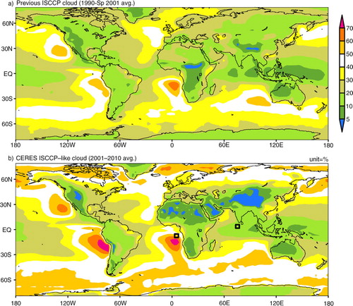
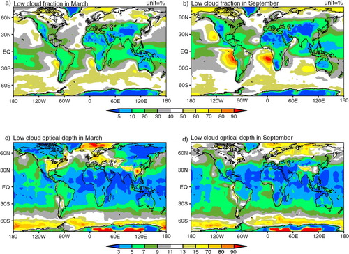
As in Chung et al. (2005), the optical depth and fraction of low, mid, high and convective clouds go into the MACR model in the present study. Figure 2 shows the CERES ISCCP-D2-like low cloud. As Fig. 2 demonstrates, both low cloud fraction and optical depth have strong spatial variability. Low cloud fraction also shows very large seasonal fluctuation.

Fig. 2 CERES ISCCP-like cloud (2001–2010 average).

3. Aerosol radiative forcing at a fixed local point

Haywood and Shine (1997), Meloni et al. (2005), Zarzycki and Bond (2010) and Samset and Myhre (2011) among others addressed local aerosol forcing (i.e. forcing at a fixed spatial point) in relation to the vertical location of aerosols. Here, we revisit the effect of aerosol vertical profile on local aerosol forcing in order to ensure consistency between local forcing and global forcing results. To do that, we look at the difference between the direct radiative effect of aerosols above low cloud heights and that of aerosols below low cloud heights, denoted as ΔRF, locally and also globally. In the local forcing computations (as shown in Figs. 3 and 4), the direct radiative effect (which refers to the forcing due to total aerosols and not aerosol change over time) is computed at two spatially different locations using the MACR model (as described in Section 2) and its annual mean value is presented. These two locations, as shown in Fig. 1b, represent aerosol downstream areas with a significant amount of low cloud in the background. One location is just south of the Indian subcontinent and has a frequent occurrence of low cloud in the winter monsoon season, when man-made aerosols from South Asia are transported southward. The other location is west of the biomass burning regions in Africa. Biomass burning aerosols are transported westward to the equatorial eastern Atlantic, where low cloud often prevails, especially in August and September (in view of the CERES ISCCP-D2-like product).

Fig. 3 Aerosol radiative forcing difference: ΔRF=RF_{2.5–3.5 km} − RF_{0.0–1.0 km}, where RF_{2.5–3.5 km} refers to the forcing with aerosols between 2.5 and 3.5 km in height. The aerosol forcing is computed with the MACR model at two different locations: 5.63°E, 6.98°S and 75.94°E, 4.19°N (see Fig. 1b for the visual illustration of the locations), and the computed forcing represents the annual mean values at the TOA level. In (a), the overcast sky refers to a 100% cloud fraction by low-level cloud. The low cloud here is assumed to extend from 1.0 to 2.0 km in height. In (c), the surface is assumed to be land with an albedo of 0.9. In (d), the overcast sky refers to a 100% cloud fraction by mid-level cloud, which is set to extend from 4.0 to 6.0 km in height.

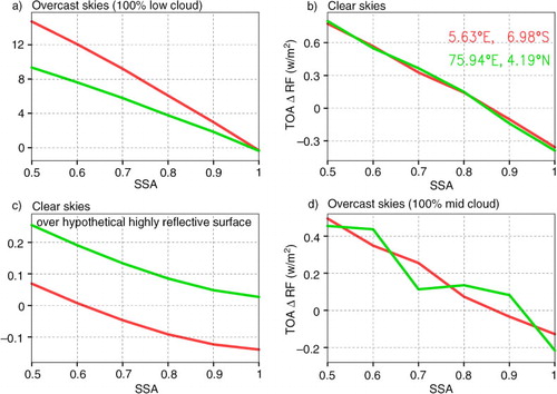
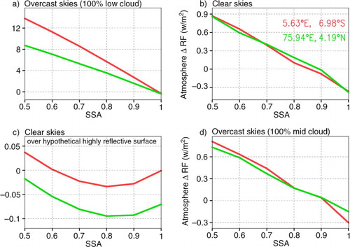
Fig. 4 Same as Fig. 3 except for the aerosol forcing in the atmosphere.

In all the forcing computations in Figs. 3 and 4, the AOD is set to 0.1 at 550 nm, the AOD Ångström Exponent 0.7, the asymmetry parameter 0.7 at 550 nm and SSA is set as wavelength independent. Non-aerosol variables, such as cloud optical depth, surface albedo, air temperature, ozone concentration and so on, are from the MACR model, and thus different between the two chosen locations. The low cloud optical depth, which is a function of calendar month in our study, ranges from 2.6 to 9.8 over the Atlantic point and ranges from 1.9 to 3.6 over the Indian point. In clear-sky experiments (Fig. 3b and 4b), cloud fraction is set to zero, while in overcast sky experiments (Fig. 3a and 4a) the low-level cloud fraction is set to 100% and the fraction of other type clouds is set to zero. In this way, we look at the effect of low cloud on aerosol forcing. When aerosols are above cloud, these aerosols are mostly above low-level cloud, and so our experiments are realistic. Low cloud is set to extend from 1.0 to 2.0 km in height. Aerosols below low cloud heights are set to extend from the surface to 1.0 km, and the aerosols above low cloud heights are set to extend from 2.5 to 3.5 km in height.

We use the TOA aerosol forcing difference between the aerosols above low cloud heights and the aerosols below low cloud heights, denoted as ΔRF, to quantify the impact of aerosol vertical profile on aerosol forcing. Please note that we apply the same AOD (i.e. 0.1) for each aerosol layer and the TOA aerosol forcing here represents the forcing due to an AOD of 0.1. Figure 3 shows that ΔRF increases as the SSA decreases. Except when the SSA is near 1.0, ΔRF is much larger in overcast skies than in clear skies, demonstrating that cloud greatly amplifies the effect of aerosol vertical profile. When the SSA is 0.8, ΔRF is 3.8–6.1 W m⁻² in overcast skies and 0.14–0.15 W m⁻² in clear skies, in which case, whether aerosols are above cloud or below induces 25–43 times as large changes of the aerosol forcing as how aerosols are vertically distributed in clear skies. In an additional set of experiments where the surface is assumed to be highly reflective with an albedo of 0.9 (Fig. 3c and 4c), ΔRF is even smaller than in clear skies. With an SSA of 0.8, ΔRF is −0.1–0.1 W m⁻². This experiment (Fig. 3c and 4c) helps to quantify the importance of aerosol vertical profile above cloud or desert. In Fig. 3d, both low-layer aerosols and upper-layer aerosols are under mid-level cloud. In this experiment, mid-cloud is the only cloud. With an SSA of 0.8, ΔRF is near 0.1 W m⁻², which is as small as ΔRF in Fig. 3c. Thus, we see that how aerosols are vertically distributed above cloud or below cloud makes very little difference in the aerosol forcing at the TOA level.

The great amplification of aerosol forcing by cloud, as demonstrated in Fig. 3a and 3b, is consistent with the previous studies such as Haywood and Shine (1997), Zarzycki and Bond (2010), Samset and Myhre (2011) and Vuolo et al. (2014). Also, Zarzycki and Bond (2010) pointed out that black carbon aerosol forcing does not change with height significantly when the aerosols are above cloud. Their finding is consistent with what we demonstrated in Fig. 3c. The uniqueness of our calculation though lies in using ΔRF instead of quantifying contribution from a single layer of aerosols as done in previous studies. Our study more directly focuses on the vertical redistribution of aerosols than previous studies. In addition, we test the effect of varying SSA instead of dealing with a specific species of aerosols such as black carbon and sulphate aerosols as in Samset and Myhre (2011). Addressing varying SSA is to address aerosol radiative forcing, as opposed to the radiative forcing of a specific aerosol species.

The sign of ΔRF is also interesting to notice. In low-cloud overcast skies, the upper-layer aerosols have a more positive forcing than the lower-layer aerosols, in view of the sign of ΔRF. In clear skies, however, ΔRF is only positive when the SSA is less than about 0.85 (Fig. 3b), which means that the upper-layer aerosols have a more positive forcing than the lower-layer aerosols for significantly absorbing aerosols (and not for scattering aerosols). A similar feature is present in mid-cloud overcast skies (Fig. 3d). In case of clear skies with a highly reflective surface, the overall magnitude of ΔRF is very small, and so we do not discuss the sign of ΔRF in depth in this case.

The aerosol forcing difference in the atmosphere gives additional insights into the TOA forcing difference. As Fig. 4a, 4b, 4d demonstrate, the TOA aerosol forcing difference between the aerosols above low cloud heights and the aerosols below low cloud heights is due mainly to the forcing difference in the atmosphere, that is, the atmospheric absorption difference. Absorbing aerosols over cloud have much stronger absorption than below cloud, because the aerosols above cloud absorb both downward solar radiation and that reflected upward from the cloud. In clear skies and mid-cloud overcast skies, ΔRF in the atmosphere becomes negative for scattering aerosols (Fig. 4b and 4d), meaning that the upper-layer aerosols have less absorption than the lower-layer aerosols. This is because the atmospheric absorption by scattering aerosols (even 100% scattering aerosols) is greater than 0 and is due to increased scattering in the atmosphere. More scattering leads to greater absorption, and lower-layer aerosols produce more scattering in the column atmosphere and greater absorption (though the magnitude of the absorption is fairly small).

4. Global aerosol radiative effect

In Section 3, we have demonstrated that whether absorbing aerosols are above cloud or below induces much larger changes of the TOA aerosol forcing than how aerosols are vertically distributed in clear skies, above cloud or below cloud. This, however, does not necessarily mean that whether absorbing aerosols are above cloud or below is also the dominating factor in determining the effect of aerosol vertical profile on global aerosol forcing, because cloud is not present everywhere and aerosols are not absorbing everywhere.

To see if the findings derived from local aerosol forcing experiments hold also for the global aerosol forcing, we use realistic AOD and SSA distributions over the globe. For AOD at 550 nm, we apply the approach in Lee and Chung (2013) who integrated monthly-mean MODIS, MISR and AERONET data. Lee and Chung (2013) nudged or adjusted combined satellite AOD towards AERONET AOD. We compute the 2001–2010 average for each calendar month at the T42 resolution. In this dataset, the observation gaps are filled by the GOCART simulation (Chin et al., 2002) as in Lee and Chung (2013). These observation data gaps are predominantly confined to the polar regions and are even fewer in polar summer.

For SSA at 550 nm, the following equation is used:where N_SSA _j is the adjusted new value of SSA at grid j; AERONET _j,i is an AERONET SSA at station location i near grid j; d _j,i is the distance between j and i; and G_SSA _j,i is the GOCART SSA at the grid box containing AERONET _j,i . Here, the AERONET data and the GOCART simulation are on the T42 grids. Through the above equation, the GOCART SSA is nudged or adjusted towards the AERONET SSA. The above equation is applied for each grid and each calendar month.

Before combining the GOCART simulation and AERONET SSAs, the 2001–2010 AERONET data average was calculated from the monthly level 2.0 data for each calendar month. The average of the AERONET SSA was AOD-weighted. Then, 550 nm SSA was obtained from the neighbouring wavelength values through linear interpolation. Please note that AERONET only gives level 2 quality SSA when AOD at 440 nm>0.4 and, therefore, many regions of the earth do not have AERONET SSA data. The T42 grid version of AERONET data was created by AOD-weighted averaging SSA data on each grid.

The GOCART SSAs were prepared as follows. We used sea salt AOD from Chin et al. (2002), and BC (black carbon), OA (Organic Aerosol), dust and sulphate AODs from the Giovanni website (http://gdata1.sci.gsfc.nasa.gov/daac-bin/G3/gui.cgi?instance_id=neespi) (GES-DISC data, 2013), which contains GOCART model output from 2000 to 2007. These AODs are monthly means at 550 nm. Then, the climatological seasonal cycle for the available data period was computed. We used these simulated AOD values to compute the simulated SSA. Before generating the SSA, we first adjusted the magnitude of the simulated AOD as follows.: BC AOD=BC AOD×1.9; OA AOD=OA AOD×0.67; and dust AOD=dust AOD×0.74. We made this adjustment in order to match the global averages in Chung et al. (2012), who constrained BC, OA and dust AODs by AERONET observations. Then, the GOCART SSA at 550 nm was computed using the following equation:BC here refers to the GOCART BC AOD. This computation was done for each grid and for each calendar month.

Even if the GOCART SSA is nudged towards the AERONET SSA, the GOCART simulation must have sizable impacts on the final SSA. To quantify the model influence in determining the effect of aerosol vertical profile on global aerosol forcing, two sets of additional GOCART SSA simulations were generated, representing lower and upper limits of absorption. These two sets were again nudged towards the AERONET SSA. In the most absorbing case, BC AOD=BC AOD×1.74; OA AOD=OA AOD×0.49; and dust AOD=dust AOD×0.74. The GOCART SSA at 550 nm was computed using the following equation: GOCART SSA=(0.14×BC+0.8×OA+1.0×sulfate+1.0×sea salt+0.96×dust)/total_AOD. The coefficients used to develop the most absorbing case, such as 0.14 (for BC SSA) are again from Chung et al. (2012) who gave the best estimates and their uncertainties. From the uncertainty range, we took the most absorbing extreme. The most absorbing case will be used in a sensitivity experiment (i.e. Exp. 1 of Table 1). In the least absorbing case (i.e. Exp. 2 of Table 1), we did not adjust the magnitude of the GOCART AOD. The GOCART SSA at 550 nm was computed using the following equation:The OA SSA of 0.98 is a common value used in climate modelling, which does not account for brown carbon sufficiently.

Table 1. The global sum of annual mean ∣ΔRF∣=∣RF_upper-RF_lower∣

	Baseline run	Exp. 1	Exp. 2	Exp. 3	Exp. 4
Range of upper aerosol layer (in km)		2.5–3.0		2.0–2.5	3.0–3.5
Range of lower aerosol layer (in km)			0.0–0.5
Global sum of ∣ΔRF∣ in clear sky portions (in W)	7.1×10^14	7.2×10^14	7.1×10^14	5.8×10^14	8.4×10^14
Global sum of ∣ΔRF∣ in low cloud only portions	4.2×10^15	4.1×10^15	4.1×10^15	3.9×10^15	4.1×10^15
Global sum of ∣ΔRF∣ below cloud (other than low cloud)	4.0×10^14	4.0×10^14	3.9×10^14	3.6×10^14	4.9×10^14

See Fig. 3 for the detailed definition of ΔRF.

The 2001–2010 average AAOD (Aerosol Absorption Optical Depth) at 550 nm is shown in Fig. 5a. This AAOD is based on our baseline SSA calculation, which lies between the most absorbing and least absorbing cases. The largest AAOD values are realised over the biomass burning regions of Africa and associated downstream areas, and also over eastern China. For AAOD to be large, AOD needs to be large and SSA needs to be small. Please note that the global AOD and SSA we have generated describes total aerosols and not anthropogenic aerosols. Aerosol forcing is due to anthropogenic aerosols and so we compute aerosol direct effect (which includes the effect of natural aerosols) hereafter. AOD and SSA observations do not distinguish natural aerosols from anthropogenic aerosols.

Fig. 5 AAOD (Absorption Aerosol Optical Depth) at 550 nm in (a). Aerosol radiative forcing difference: ΔRF=RF_{2.5–3.0 km} − RF_{0.0–0.5 km}, in (b) and (c). The aerosol forcing is computed with the MACR model, and the computed forcing represents the 2001–2010 mean values at the TOA level. Realistic 3D clouds from satellite observations are used in (c). These clouds are removed in (b).

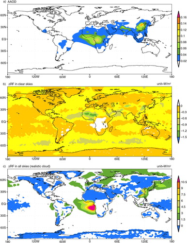
Figure 5b shows the global distribution of ΔRF in clear skies. The baseline SSA is used here. Note that the lower-layer aerosols are set to extend from the surface to 0.5 km, and the upper-layer aerosols are set to extend from 2.5 to 3.0 km in height here. This aerosol layer thickness is realistic, given the finding by Devasthale and Thomas . (2011), who showed aerosol layers to be less than 1-km thick in most cases. The clear-sky experiment is conducted by removing all of the clouds in the model. As the figure shows, ΔRF is mostly negative and its amplitude rarely exceeds 1.0 W m⁻². ΔRF is slightly positive over the biomass burning regions of Africa because the associated SSA is quite low in these regions.

Figure 5c displays the global distribution of ΔRF in all skies (i.e. skies with realistic clouds). The global cloud data is as described in Section 2. Here, low cloud is set to extend from 0.5 to 2.0 km in height and mid cloud from 3.5 to 6.0 km as in Chung et al. (2005). Thus, low-layer aerosols are below the low cloud and upper-layer aerosols are between the low cloud and the mid cloud. ΔRF is positive and large over the outflow of the African biomass burning aerosols off the coast, while slightly negative over the deserts, North America and the Eastern Siberia. ΔRF in all skies includes ΔRF in clear-sky pixel/times. The real contrast of clear-sky ΔRF is ΔRF in overcast skies, as shown in Fig. 6.

Fig. 6 Aerosol radiative forcing difference: ΔRF=RF_{2.5–3.0 km} − RF_{0.0–0.5 km}. Realistic 3D clouds as in Fig. 5c are expanded in fraction to have a 100% cloud fraction collectively in a). In b), the fraction of low cloud is set to 100% while other clouds are zeroed. In c), the low cloud is zeroed and other clouds are expanded in fraction to have a 100% cloud fraction collectively.

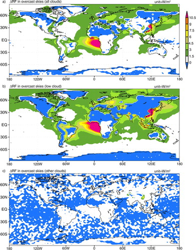
First, as shown in Fig. 6a, we generate the overcast sky by increasing the fractions of all cloud types while maintaining the ratio of the fraction of a cloud type to that of another cloud type in each grid cell. In Fig. 6b, the low cloud fraction is increased to a 100% while the other cloud types are zeroed. In contrast, the low cloud is set to zero while the other cloud types collectively make an overcast sky in Fig. 6c. Figure 6a is similar to Fig. 6b overall, whereas Fig. 6c differs greatly from Fig. 6a and 6b. These results indicate that the effect of cloud is mainly through that of low cloud. The most salient feature of ΔRF in the low-cloud overcast skies (Fig. 6b) is large values over East Asian outflow, as well as over the outflow of the African biomass burning aerosols off the coast.

In Table 1, we quantify the contribution of four aspects of the aerosol vertical profile to the global aerosol direct effect. These four aspects are: (a) vertical profile in clear sky, (b) vertical profile above low cloud, (c) vertical profile below cloud (other than low cloud) and (d) whether cloud is above low cloud or below. These four aspects collectively describe most realistic aerosol vertical profile scenarios since aerosols rarely reach mid-cloud heights or higher (especially for man-made aerosols). For instance, aerosols from South Asia are normally below 3.5 km (Ramanathan et al., 2001), and smoke pollution from central-west Africa was observed to be primarily below 4 km (de Graaf et al., 2012). An extensive analysis of CALIPSO data (Devasthale and Thomas, 2011) also shows that aerosols are in the low layers.

Table 1 demonstrates that whether aerosols are above cloud or below controls 70–80% of the effect of aerosol vertical profile on the global aerosol radiative effect. In the baseline run, the global sum of ∣ΔRF∣ just in the low-cloud only portion (i.e. low cloud without other clouds) is 4.2×10¹⁵ W, which quantifies the uncertainty of the global aerosol direct effect due to the uncertainty in whether aerosols are above cloud or below. This is compared to 7.1×10¹⁴ W in the clear sky portions, and 4.0×10¹⁴ W below cloud (below mid or high cloud, or below convective cloud top). The effect of aerosol vertical distribution above cloud (and no additional cloud above the aerosols) can be estimated by the variation of ∣ΔRF∣ in the low-cloud only portions from the baseline run to Exp. 3 and Exp.4, which is about 3.0×10¹⁴ W. Thus, whether aerosols are above low cloud (and not below other clouds) or below makes up (i.e. 75%). In the case of Exp. 3, whether aerosols are above low cloud or below makes up 77%, and this percentage goes down to 73% in the case of Exp. 4. In Exp. 1 and Exp. 2 (experiments about GOCART SSA uncertainty), the results are very similar to those of the baseline run. Thus, we conclude that whether aerosols are above cloud or below controls about 70–80% of the effect of aerosol vertical profile on the global aerosol radiative effect.

The contribution of whether aerosols are above cloud or below to the global aerosol direct effect comes almost equally from the below-cloud aerosols and from the above-cloud aerosols (not shown). In contrast, Zarzycki and Bond (2010) and Vuolo et al. (2014) demonstrated that black carbon aerosol forcing efficiency increases significantly from the below-cloud height to the above-cloud height. Our study uses realistic SSA values for total aerosols as opposed to just treating black carbon, and this causes the difference between our study and the previous studies. Our study shows that accurately estimating the global aerosol direct effect relies on accurately quantifying the amount of aerosols below and above cloud (instead of just dealing with above-cloud aerosols).

5. Conclusion and discussion

In the present study, we have demonstrated that whether aerosols are above low cloud or below determines 70–80% of the effect of aerosol vertical profile on the global aerosol radiative effect. The remaining 20–30% comes from how aerosols are vertically distributed in clear skies, above cloud or below cloud. The order of influence is as follows: whether aerosols are above low cloud or below >> how aerosols are vertically distributed in clear skies > how aerosols are vertically distributed below cloud > how aerosols are vertically distributed above cloud. In the computations, we did not consider aerosols at the height of mid cloud or above, since such elevated aerosols are not common, especially for anthropogenic particles. We did not account for aerosol vertical distribution within low cloud either, because low clouds are typically shallow.

We have also shown that the contribution from whether aerosols are above low cloud or below is mainly over East Asian outflow, and the outflow of the African biomass burning aerosols off the coast. Thus, accurately determining the fraction of aerosol amount above low cloud is particularly important over these regions, if one attempts to estimate the global aerosol direct effect. The CALIOP lidar is a very effective instrument to retrieve aerosol amount over cloud, while ground-based lidars can be used to determine the aerosol amount below cloud. Thus, we advise scientists to combine CALIOP lidar data and ground-based lidar data to observationally constrain the fraction of aerosol amount above low cloud and that below low cloud, especially over these regions. Note that aerosols below low cloud contribute as much to the global aerosol effect as aerosols above low cloud. Thus, one should not overlook aerosols below low cloud.

While we have demonstrated that whether aerosols are above low cloud or below is an important issue to the global aerosol radiative effect, this issue is likely even more important to the global aerosol direct radiative forcing (i.e. aerosol direct forcing due to anthropogenic aerosols). This is because the effect of aerosol vertical distribution in clear skies is very large over the deserts (Fig. 5b). Dust can be considered natural, and so the uncertainty in clear-sky aerosol vertical distribution plays a lesser role in uncertainty in the global aerosol direct radiative forcing than in uncertainty in the global aerosol direct radiative effect.

6. Acknowledgement

The National Research Foundation of Korea (NRF-2013R1A1A2005855) supported this research.

References

- Chin M. , Ginoux P. , Kinne S. , Torres O. , Holben B. N. , co-authors . Tropospheric aerosol optical thickness from the GOCART model and comparisons with satellite and sun photometer measurements. J. Atmos. Sci. 2002; 59: 461–483.
- Chung C. E. , Ramanathan V. , Decremer D . Observationally constrained estimates of carbonaceous aerosol radiative forcing. Proc. Nat. Acad. Sci. 2012; 109: 11624–11629.
- Chung C. E. , Ramanathan V. , Kim D. , Podgorny I. A . Global anthropogenic aerosol direct forcing derived from satellite and ground-based observations. J. Geophys. Res. 2005; 110: D24207.
- Dee D. P. , Uppala S. M. , Simmons A. J. , Berrisford P. , Poli P. , co-authors . The ERA-Interim reanalysis: configuration and performance of the data assimilation system. Q. J. Roy. Meteorol. Soc. 2011; 137: 553–597.
- de Graaf M. , Tilstra L. G. , Wang P. , Stammes P . Retrieval of the aerosol direct radiative effect over clouds from spaceborne spectrometry. J. Geophys. Res. Atmos. 2012; 117: D07207.
- Devasthale A. , Thomas M. A . A global survey of aerosol–liquid water cloud overlap based on four years of CALIPSO–CALIOP data. Atmos. Chem. Phys. 2011; 11: 1143–1154.
- GES-DISC data. Giovanni—GES-DISC Interactive Online Visualization Analysis Infrastructure. 2013. GES DISC: Goddard Earth Sciences, Data and Information Services Center.
- Haywood J. M. , Shine K. P . Multi-spectral calculations of the direct radiative forcing of tropospheric sulphate and soot aerosols using a column model. Q. J. Roy. Meteorol. Soc. 1997; 123: 1907–1930.
- Kim D. , Ramanathan V . Solar radiation budget and radiative forcing due to aerosols and clouds. J. Geophys. Res. 2008; 113: D02203.
- Lee K. , Chung C. E . Observationally-constrained estimates of global fine-mode AOD. Atmos. Chem. Phys. 2013; 13: 2907–2921.
- Ma X. , Yu F. , Luo G . Aerosol direct radiative forcing based on GEOS-Chem-APM and uncertainties. Atmos. Chem. Phys. 2012; 12: 5563–5581.
- Meloni D. , di Sarra A. , Di Iorio T. , Fiocco G . Influence of the vertical profile of Saharan dust on the visible direct radiative forcing. J. Quant. Spectrosc. Radiat. Transfer. 2005; 93: 397–413.
- Müller D. , Veselovskii I. , Kolgotin A. , Tesche M. , Ansmann A. , co-authors . Vertical profiles of pure dust and mixed smoke-dust plumes inferred from inversion of multiwavelength Raman/polarization lidar data and comparison to AERONET retrievals and in situ observations. Appl. Opt. 2013; 52: 3178–3202.
- Myhre G. , Samset B. H. , Schulz M. , Balkanski Y. , Bauer S. , co-authors . Radiative forcing of the direct aerosol effect from AeroCom Phase II simulations. Atmos. Chem. Phys. 2013b; 13: 1853–1877.
- Myhre G. , Shindell D. , Bréon F.-M. , Collins W. , Fuglestvedt J. , co-authors . Stocker T. F. , Qin D. , Plattner G.-K. , Tignor M. , Allen S. K. , Boschung J. , co-authors . Anthropogenic and natural radiative forcing. Climate Change 2013: The Physical Science Basis. Contribution of Working Group I to the Fifth Assessment Report of the Intergovernmental Panel on Climate Change. 2013a; Cambridge, United Kingdom: Cambridge University Press. 659–740.
- Noh Y. M. , Lee H. , Mueller D. , Lee K. , Shin D. , co-authors . Investigation of the diurnal pattern of the vertical distribution of pollen in the lower troposphere using LIDAR. Atmos. Chem. Phys. 2013; 13: 7619–7629.
- Ramana M. V. , Ramanathan V. , Feng Y. , Yoon S. C. , Kim S. W. , co-authors . Warming influenced by the ratio of black carbon to sulphate and the black-carbon source. Nat. Geosci. 2010; 3: 542–545.
- Ramanathan V. , Crutzen P. J. , Lelieveld J. , Mitra A. P. , Althausen D. , co-authors . Indian ocean experiment: an integrated analysis of the climate forcing and effects of the great Indo-Asian haze. J. Geophys. Res. 2001; 106: 28371–28398.
- Rossow W. B. , Schiffer R. A . Advances in Understanding Clouds from ISCCP. Bull. Am. Meteorol. Soc. 1999; 80: 2261–2287.
- Samset B. H. , Myhre G . Vertical dependence of black carbon, sulphate and biomass burning aerosol radiative forcing. Geophys. Res. Lett. 2011; 38: L24802.
- Sun M. , Doelling D. R. , Raju R. I. , Nguyen L. C. , Loeb N. G . The CERES ISCCP-D2 like cloud and radiative property data product. AGU Fall Meeting Abstracts. 2010; 893.
- Vuolo M. R. , Schulz M. , Balkanski Y. , Takemura T . A new method for evaluating the impact of vertical distribution on aerosol radiative forcing in general circulation models. Atmos. Chem. Phys. 2014; 14: 877–897.
- Winker D. M. , Pelon J. , Coakley J. A. , Ackerman S. A. , Charlson R. J. , co-authors . The CALIPSO mission: a global 3D view of aerosols and clouds. Bull. Am. Meteorol. Soc. 2010; 91: 1211–1229.
- Yang S.-K. , Zhou S. , Miller A. J . SMOBA: a 3-dimensional daily ozone analysis using SBUV/2 & TOVS measurements. 2006; Washington: National Oceanic and Atmospheric Administration.
- Zarzycki C. M. , Bond T. C . How much can the vertical distribution of black carbon affect its global direct radiative forcing?. Geophys. Res. Lett. 2010; 37: L20807.