Impacts of land use and land cover changes on biogenic emissions of volatile organic compounds in China from the late 1980s to the mid-2000s: implications for tropospheric ozone and secondary organic aerosol

Abstract

Based on the MEGAN (Model of Emissions of Gases and Aerosols from Nature) module embedded within the global chemical transport model (GEOS-Chem), we estimate the changes in emissions of biogenic volatile organic compounds (BVOCs) and their impacts on surface-layer O₃ and secondary organic aerosols (SOA) in China between the late 1980s and the mid-2000s by using the land cover dataset derived from remote sensing images and land use survey. The land cover change in China from the late 1980s to the mid-2000s can be characterised by an expansion of urban areas (the total urban area in the mid-2000s was four times that in the late 1980s) and a reduction in total vegetation coverage by 4%. Regionally, the fractions of land covered by forests exhibited increases in southeastern and northeastern China by 10–30 and 5–15%, respectively, those covered by cropland decreased in most regions except that the farming–pastoral zone in northern China increased by 5–20%, and the factions of grassland in northern China showed a large reduction of 5–30%. With changes in both land cover and meteorological fields, annual BVOC emission in China is estimated to increase by 11.4% in the mid-2000s relative to the late 1980s. With anthropogenic emissions of O₃ precursors, aerosol precursors and aerosols fixed at year 2005 levels, the changes in land cover and meteorological parameters from the late 1980s to the mid-2000s are simulated to change the seasonal mean surface-layer O₃ concentrations by −4 to +6 ppbv (−10 to +20%) and to change the seasonal mean surface-layer SOA concentrations by −0.4 to +0.6 µg m⁻³ (−20 to +30%) over China. We find that the decadal changes in meteorological parameters had larger collective effects on BVOC emissions and surface-layer concentrations of O₃ and SOA than those in land cover and land use alone. We also perform a sensitivity simulation to compare the impacts of changes in anthropogenic emissions on concentrations of O₃ and SOA with those of the changes in meteorological parameters and land cover.

• biogenic emissions
• land cover and land use
• tropospheric O₃
• secondary organic aerosol

1. Introduction

Volatile organic compounds (VOCs) in the atmosphere are important for air quality and climate. Biogenic isoprene (C₅H₈) is an important precursor of tropospheric O₃ (Arneth et al., 2011), and biogenic isoprene and monoterpenes (C₁₀H₁₆) are major sources of secondary organic aerosol (SOA) (Carslaw et al., 2010). Ozone and SOA are both air pollutants that can influence the Earth's radiation budget (IPCC, 2007). Present-day emissions of biogenic volatile organic compounds (BVOCs) are found to be comparable in magnitude to anthropogenic emissions on the global scale (Guenther et al., 1995, 2006). Quantification of changes in BVOCs on different time scales is important for understanding changes in air quality and climate.

Changes in BVOC emissions are influenced by changes in meteorological conditions (e.g. temperature, radiation and soil moisture) as well as the changes in land cover and land use (LCLU). On decadal time scale, changes in LCLU result from both climate change (e.g. changes in temperature, precipitation and CO₂ concentration) and human activities such as agriculture expansion, deforestation or afforestation, and urbanisation. The commonly used tools to account for climate-driven changes in vegetation are dynamic vegetation models (Sanderson et al., 2003; Wu et al., 2012). To account for the impacts of both climate change and human activities, previous studies usually combined changes in natural vegetation calculated by dynamic vegetation models with those in crops, pastures and urban land use based on satellite retrieval and historical statistic data, or with projected future anthropogenic land use changes compiled by the Intergovernmental Panel on Climate Change (IPCC) (Ganzeveld et al., 2010; Lathiere et al., 2010; Hurtt et al., 2011; Wu et al., 2012). Ganzeveld et al. (2010) estimated 2000–2050 changes in natural vegetation and anthropogenic land use with the Integrated Model to Assess the Global Environment (IMAGE) and reported that the simulated annual global isoprene emission would decrease by 12% over 2000–2050. Lathiere et al. (2010) combined the natural vegetation distribution derived from the dynamic vegetation model (SDGVM) with the crop map based on satellite retrieval and historical statistic data to study the changes in BVOC emissions over 1901–2002. They found that anthropogenic land use was very influential on simulated biogenic emissions; relative to the annual global isoprene emission simulated with natural vegetation alone, consideration of both natural vegetation and anthropogenic croplands led to a reduction in global isoprene emission by 8% in 1901 and by 16% in 2002. Wu et al. (2012) reported that the annual global isoprene emission was simulated to decrease by 5% over 2000–2050 with both climate-driven vegetation change and the agricultural land use under the IPCC A1B scenario.

Since the simulated land cover changes exhibited large differences in different dynamic vegetation models (Cramer et al., 2001), a growing number of studies on BVOC emissions used LCLU datasets derived from satellite observation and land survey (Gulden et al., 2008; Smiatek et al., 2009; Leung et al., 2010; Zemankova and Brechler, 2010; Zheng et al., 2010; Wang et al., 2011a). Gulden et al. (2008) compared simulated 1993–1998 biogenic emissions over Texas, USA, using survey-derived plant functional type (PFT) with those using satellite-derived PFT, and found that the statewide mean monthly BVOC emission from the former approach was three times the value from the latter one. Smiatek et al. (2009) simulated the BVOC emissions in an extended European area for 4 yr (1997, 2000, 2001 and 2003) by using a satellite-derived land use map and leaf area index in a semi-empirical BVOC model (SeBVOC), and reported that the monthly BVOC emissions in May to September exhibited interannual variation of about ±10% in forest areas. Zheng et al. (2010) utilised high-resolution (3 km×3 km) land cover dataset developed on the basis of the vegetation map of Guangdong and the land use database provided by the Domestic Land Use Information Center of Guangdong Province in the Global Biosphere Emissions and Interactions System model (GloBEIS) to estimate the spatial distribution and seasonal variation of BVOCs in the Pearl River Delta region of China for 2006. Leung et al. (2010) used satellite-based land cover maps from the Hong Kong Special Administrative Region government report to calculate BVOC emissions in Hong Kong, and found that annual BVOC emission increased by 7% over 1995–2006 as a result of the increases in areas covered by forests. These studies, however, were mostly focused on BVOC emissions on seasonal to interannual time scales.

The changes in BVOC emissions on different time scales have been shown to influence tropospheric O₃ and SOA concentrations in China. By using the Weather Research and Forecasting coupled with Chemistry (WRF-Chem)/Model of Emissions of Gases and Aerosols from Nature (MEGAN) model, Situ et al. (2013) estimated the impacts of seasonal variations in BVOCs on surface-layer O₃ over the Pearl River Delta region for year 2010 and reported that the impact of BVOC emissions on the surface ozone peak was about 10 ppbv (3 ppbv) on average with a maximum value of 34 ppbv (24.8 ppbv) in summer (autumn), as the concentrations simulated with BVOC emissions were compared with those simulated without BVOC emissions. By using the GEOS-Chem/MEGAN model, Fu and Liao (2012) reported that the interannual variations in BVOCs over 2001–2006 led to differences in simulated summertime surface-layer O₃ and SOA concentrations in China by 2–5%. Wu et al. (2012) predicted that the changes in natural vegetation and anthropogenic land use over 2000–2050 would change summertime afternoon-averaged surface-layer O₃ concentrations by ±5 ppbv over China and would increase the summertime surface-layer SOA concentrations by about 0.5 µg m⁻³ in Eurasia. Tai et al. (2013) also showed that the projected changes in cropland over 2000–2050 following the IPCC A1B scenario would lead to changes in summertime surface-layer O₃ concentration by ±4 ppbv over East Asia.

The purpose of our study is to quantify the changes in BVOC emissions in China between the late 1980s and the mid-2000s and the impacts of such changes in BVOCs on concentrations of surface-layer O₃ and SOA, using the global chemical transport model GEOS-Chem/MEGAN together with the investigated and satellite-derived land cover datasets. We also compare the impacts of changes in anthropogenic emissions on concentrations of O₃ and SOA with those of the changes in meteorological parameters and land cover over the studied time period. This study is an extension of our previous work (Fu and Liao, 2012), in which we investigated the interannual variations in BVOC emissions in China as a result of the interannual variations in meteorological parameters and land cover over 2001–2006.

Section 2 describes the model and simulations, including the LCLU datasets used in simulations. In Section 3, we present changes in LCLU in China from the late 1980s to the mid-2000s. Section 4 shows the simulated changes in biogenic emissions in China during the studied time period and discusses the roles of decadal changes in meteorology and/or land cover in simulated changes in biogenic emissions. The simulated decadal changes in surface-layer concentrations of O₃ and SOA are examined in Section 5. Section 6 compares, over the studied time period, the simulated impacts on concentrations O₃ and SOA as a result of the changes in anthropogenic emissions alone with those caused by changes in meteorological parameters and land cover.

2. Methods

2.1. Model description

We simulate BVOC emissions using the global three-dimensional chemical transport model GEOS-Chem (v8-03-02, http://acmg.seas.harvard.edu/geos/) driven by the GEOS-4 assimilated meteorological fields from the Goddard Earth Observing System (GEOS) of the NASA Global Modeling and Assimilation Office (GMAO). The version of the model we use has a horizontal resolution of 2° latitude by 2.5° longitude and 30 vertical layers up to 0.01 hPa. The GEOS-Chem model has fully coupled simulation of ozone–NO_x–hydrocarbon chemistry (Bey et al., 2001) and aerosols (Park et al., 2003, 2004; Alexander et al., 2005; Fairlie et al., 2007) including sulphate (), nitrate (), ammonium (), organic carbon (OC), black carbon (BC), sea salt and mineral dust. SOA formation considers the oxidation of isoprene (Henze and Seinfeld, 2006), monoterpenes and other reactive VOCs (ORVOCs) (Liao et al., 2007), and aromatics (Henze et al., 2008). Wet deposition scheme in GEOS-Chem follows that in Liu et al. (2001). The dry deposition velocities are calculated locally dependent on species properties, surface type and meteorological conditions. To see the impacts of biogenic emissions on simulated O₃ and SOA, the Olson land cover classes (Olson, 1992) are used to calculate dry deposition and are assumed not to change in this study.

Biogenic VOC emissions in GEOS-Chem are calculated using the MEGAN module (Guenther et al., 2006), which was implemented into the GEOS-Chem by Barkley et al. (2011). Biogenic emissions of 12 chemical species are simulated, including isoprene, monoterpenes, α-pinene, β-pinene, limonene, myrcene, sabinene, 3-carene, ocimene, methylbutenol (MBO), acetone and the lumped≥C3 alkenes.

2.2. Land cover datasets

The National Land Cover Dataset (NLCD) used in this study was produced by Chinese Academy of Science and was obtained from the Data Sharing Infrastructure of Earth System Science (http://www.geodata.cn/Portal/index.jsp). The NLCD was derived from the Landsat Thematic Mapper (TM) and Enhanced Thematic Mapper (ETM) images, mainly through visual interpretation based on the experiences of experts from disciplines of agriculture, forestry and geography. The information used for interpretation included spectral reflectance, texture, terrain and digital elevation model (DEM) (Liu, 1996; Liu and Buhe, 2000; Liu et al., 2001, 2002 2003, 2005a 2005b). The dataset is available for four time periods of the late 1980s, mid-1990s, late 1990s and mid-2000s, which has been validated by extensive field surveys (Liu, 1996; Liu et al., 2005a, 2005b 2006, 2010; Wu et al., 2008). We chose to use datasets of the late 1980s and mid-2000s to examine decadal changes in land cover and BVOCs. The overall accuracy of datasets for the late 1980s was reported to be 92.9% for land cover classification and 97.6% for land cover change detection; for forest, grassland, cropland and built-up areas, the accuracies were 90.1, 88.1, 94.9 and 96.3%, respectively (Liu et al., 2005a, 2005b). The overall interpretation accuracy of NLCD datasets in mid-2000s was reported to be over 95%, in which the accuracy was 99% for cropland and 98% for grassland, forest and built-up area (Liu et al., 2010).

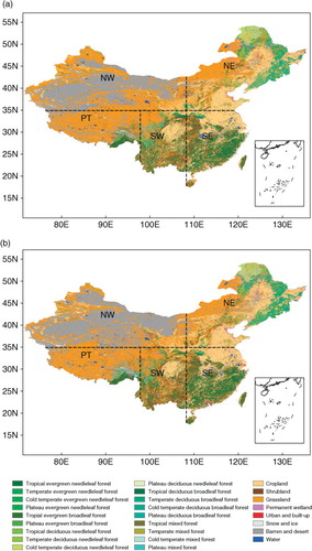
The NLCD used a hierarchical classification system, consisting of six land cover classes at Level I and 25 land cover classes at Level II. We aggregate the 25 land cover classes of Level II datasets into nine land cover types including forest, crop, shrub, grass, wetland, urban, barren land and desert, snow and ice, and water. Then we classify the forest as evergreen broadleaf trees, deciduous broadleaf trees, evergreen needleleaf trees, deciduous needleleaf trees and mixed forest according to the 1:1 000000 vegetation map of China (Hou, 2001; Zhang, 2007). The classification of forest also considers the four typical climatic zones (tropical, temperate, cold-temperate, plateau climatic zones) in China, which are obtained based on the observed temperature and precipitation datasets at 752 weather stations in China over 1971–2000 (http://cdc.cma.gov.cn/), following the standards of regionalisation in China-climatic zones and climatic regions (CNIS, 1998) [See Fu and Liao (2012) for more details]. As a result, a new land cover map with 26 land cover types is developed, which includes 18 types of forest, shrub, grass, crop, wetland, as well as four non-vegetated land types (barren land and desert, snow and ice, urban, and water). The distributions of 26 land cover types in China in the late 1980s and mid-2000s based on the NLCD dataset are shown in Fig. 1.

Fig. 1 Distributions of land cover and land use types in China in (a) the late 1980s and (b) the mid-2000s. The regions of China examined in this study are also shown, including northeastern (NE, 35.00°–53.00°N, 108.75°–136.25°E), southeastern (SE, 17.00°–35.00°N, 108.75°–123.75°E), northwestern (NW, 35.00°–49.00°N, 73.75°–108.75°E), southwestern (SW, 21.00°–35.00°N, 96.25°–108.75°E), and plateau (PT, 27.00°–35.00°N, 76.25°–96.25°E) regions.

The datasets of leaf area index LAI (m² m⁻²) in China are obtained from the Moderate Resolution Imaging Spectroradiometer (MODIS) products (MOD15A2 version 5, https://lpdaac.usgs.gov/products/modis_products_table/) of monthly mean LAI with resolutions of 8-d and 1 km. The MODIS LAI datasets are available from 2001 to present. The monthly mean LAI is then averaged over the fraction of land area covered by vegetation within each grid cell (referred to as LAIv) following the approach of Guenther et al. (2006) and Müller et al. (2008).

2.3. Calculation of biogenic emissions

The biogenic emissions (E) are calculated as1 where E ₀ (µg C m⁻² h⁻¹) is the emission factor representing the emission of a compound into the canopy at standard conditions (air temperature=303 K, photosynthetic active radiation (PAR)=1500 µmol m⁻² s⁻¹, LAI=5 m² m⁻²), which is multiplied by emission activity factors to represent changes in the emission rate attributing to changes in canopy environment γ_CE, leaf age γ_age, and soil moisture γ_SM. We do not consider the effect of soil moisture and the extra production or loss of BVOCs in the vegetation canopy in this work by setting γ _SM=1 and ρ=1. γ _CE is a function of temperature, PAR, and LAI, which is parameterised differently for different biogenic species (Guenther et al., 2006).

The emission factor E ₀ of a biogenic compound (for example, isoprene or monoterpenes) in each gird cell is calculated as2 where E _fi (µg C gdm⁻¹ h⁻¹) is the specific emission factor prescribed for the ith PFT in the grid cell under standard conditions, s _i (gdm m⁻², dm represents dry matter) is the specific leaf weight of the ith PFT, and ω _i is the fraction of the grid area covered by the ith PFT. The values of E _fi and s _i for isoprene and monoterpenes used in our study are compiled from previous studies (Guenther et al., 1995; Levis et al., 2003; Bai et al., 2006; Lathiere et al., 2006) and are listed in Table 1. For other species of BVOCs, we use the emission factors given by Guenther et al. (2006). Note that we assume that the vegetation composition (in terms of biogenic emission rates) for each PFT remained unchanged from the late 1980s to the mid-2000s since the MEGAN scheme resolves the PFTs but not detailed plant species. The model's performance in simulating the biogenic VOC emissions in China has been evaluated in Fu and Liao (2012) by comparisons with other studies.

Table 1. Isoprene and monoterpene emission factors and specific leaf weight (SLW) used in this study

		Emission factors (E fi, µg C gdm^−1 h^−1)
Climatic zones	Land cover types	isoprene	monoterpenes	SLW^a (s)(gdm m^−2)	References^b
Cold-temperate zone	Cold-temperate Evergreen Needleleaf trees (CoTeEN)	8	2.4	150	1,2
	Cold-temperate Deciduous Needleleaf trees (CoTeDN)	8	2.4	150	1,2
	Cold-temperate Deciduous Broadleaf trees (CoTeDB)	8	2.4	150	1,2
	Cold-temperate Mixed forest (CoTeMixed)	8	1.2	125	1,2
Temperate zone	Temperate Evergreen Needleleaf trees (TeEN)	16	2.4	150	1,2
	Temperate Deciduous Needleleaf trees (TeDN)	16	2.4	150	1,2
	Temperate Deciduous Broadleaf trees (TeDB)	45	1.2	100	1,2
	Temperate Mixed forest (TeMixed)	24	0.8	100	1,2
Tropical zone	Tropical Evergreen Needleleaf trees (TrEN)	24	0.8	125	1,2
	Tropical Deciduous Needleleaf trees (TrDN)	24	0.8	125	1,2
	Tropical Deciduous Broadleaf trees (TrDB)	24	0.8	125	3
	Tropical Evergreen Broadleaf trees (TrEB)	24	0.8	125	3
	Tropical Mixed forest (TrMixed)	24	0.8	125	1,2
Plateau zone	Plateau Evergreen Needleleaf trees (PlEN)	16	2.4	150	1,2
	Plateau Evergreen Broadleaf trees (PlEB)	16	0.8	125	1,2
	Plateau Deciduous Broadleaf trees (PlDB)	45	0.8	100	1,2
	Plateau Deciduous Needleleaf trees (PlDN)	16	2.4	150	1,2
	Plateau Mixed forest (PlMixed)	24	0.8	100	1,2
	Shrubland	20	0.8	125	1,2
	Grassland	5	0.8	125	2,4
	Cropland	5	0.2	125	1,2
	Permanent wetland	8	0.4	150	1
	Snow and ice	0	0	0
	Urban and built-up	0	0	0
	Barren and desert	0	0	0
	Water	0	0	0

^aSLW: leaf dry weight per unit leaf area (gdm m⁻²), which is the inverse of specific leaf area (SLA, m⁻² gdm).

^b1. Guenther et al. (1995); 2. Lathiere et al. (2006); 3. Levis et al. (2003); 4. Bai et al. (2006).

2.4. Numerical experiments

We perform the following simulations using the GEOS-Chem/MEGAN, focusing on the changes in BVOC emissions and concentrations of tropospheric O₃ and SOA between the late 1980s and the mid-2000s. The simulations are designed to quantify the roles of changes in LCLU and/or meteorological parameters in simulated changes in BVOC emissions and concentrations of tropospheric O₃ and SOA (Table 2):

1. CTRL_1980s: Control simulation for the late 1980s driven by the GEOS-4 assimilated meteorological fields of 1986–1988. Distributions of PFTs are those in the late 1980s. Anthropogenic emissions of O₃ precursors, aerosol precursors, and aerosols are fixed at the year 2005 levels.

2. CTRL_2000s: Control simulation for the mid-2000s driven by the GEOS-4 assimilated meteorological fields of 2004–2006. Distributions of PFTs are those in the mid-2000s. Anthropogenic emissions of O₃ precursors, aerosol precursors, and aerosols are fixed at the year 2005 levels.

3. SENS_LCLU: Sensitivity simulation to examine the impacts of decadal land cover change on BVOC emissions and concentrations of O₃ and SOA by comparing with simulation CTRL_1980s. Meteorological fields are the same as those in simulation CTRL_1980s, but the distributions of PFTs are set to those in the mid-2000s. Anthropogenic emissions of O₃ precursors, aerosol precursors, and aerosols are fixed at the year 2005 levels.

4. SENS_MET: Sensitivity simulation to examine the role of changes in meteorological parameters in simulated decadal changes in BVOC emissions and concentrations of O₃ and SOA by comparing with simulation CTRL_1980s. The distributions of PFTs are the same as those in simulation CTRL_1980s, but this simulation is driven by meteorological fields of 2004–2006. Anthropogenic emissions of O₃ precursors, aerosol precursors, and aerosols are fixed at the year 2005 levels.

5. SENS_ANTH: Sensitivity simulation to examine the role of changes in anthropogenic emissions in simulated decadal changes in concentrations of O₃ and SOA by comparing with simulation CTRL_2000s. The distributions of PFTs and meteorological fields are the same as those in simulation CTRL_2000s, but the anthropogenic emissions of O₃ precursors, aerosol precursors, and aerosols are set to year 1985 values.

Table 2. Summary of the simulations in this study

		Vegetation parameters
Simulations	GEOS4 Meteorology	Land cover	Leaf area index	Anthropogenic emissions
(1) CTRL_1980s	1986–1988	Late 1980s	Averaged over 2001–2006	2005
(2) CTRL_2000s	2004–2006	Mid-2000s	Averaged over 2001–2006	2005
(3) SENS_LCLU	1986–1988	Mid-2000s	Averaged over 2001–2006	2005
(4) SENS_MET	2004–2006	Late 1980s	Averaged over 2001–2006	2005
(5) SENS_ANTH	2004–2006	Mid-2000s	Averaged over 2001–2006	1985

It should be noted that the LAI datasets from MODIS product are not available for the late 1980s. The averaged LAI from MODIS over 2001–2006 are used in all the simulations listed above. To isolate the effect of changes in biogenic emissions on simulated O₃ and SOA, anthropogenic emissions of O₃ precursors, aerosol precursors, and aerosols are fixed at the year 2005 levels in simulations (1)–(4). Global emissions of ozone precursors, aerosol precursors, and aerosols in the GEOS-Chem model are taken from the EDGAR 3.2 global inventory for 2000 (Olivier and Berdowski, 2001), while anthropogenic emissions of non-methane VOCs are from the GEIA inventory for 1985 (Piccot et al., 1992). These default inventories are scaled for years 1985 and 2005 on the basis of economic data (Yang et al., 2014). The anthropogenic emissions in Asia domain are taken from David Streets’ emission inventory (Streets et al., 2003, 2006) and are scaled to years 1985 and 2005.

For presentation of model results, the China domain is divided into five regions, including northeastern (NE, 35.00°–53.00°N, 108.75°–136.25°E), southeastern (SE, 17.00°–35.00°N, 108.75°–123.75°E), northwestern (NW, 35.00°–49.00°N, 73.75°–108.75°E), southwestern (SW, 21.00°–35.00°N, 96.25°–108.75°E), and plateau regions (PT, 27.00°–35.00°N, 76.25°–96.25°E), which are also shown in Fig. 1.

3. Changes in land cover and land use from the late 1980s to the mid-2000s

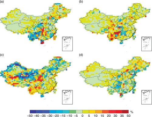
Changes in LCLU from the 1980s to the mid-2000s reflected the rapid urbanisation over the past decades. Based on the datasets we use, the total urban area in the mid-2000s was about four times that in the late 1980s, which was consistent with the change of urban area surveyed by National Bureau of Statistics of China (Qiu, 2006). Simultaneously, the total area covered by vegetation exhibited a reduction of 4%, and the area of desert and bare land increased by 11%. Such changes in desert areas between those two time periods were also reported in Wang et al. (2008a). Here we analyse the decadal changes in the four major vegetation types. Figure 2 shows the changes in fractions of each 1°×1° grid cell covered by forests, shrubs, grass, and crops from the late 1980s to the mid-2000s. The areas covered by forests increased in the temperate regions of China; the fractions of forests in NE increased by 5–15% and those over Tsinling and Nanling Mountains increased by 10–30% (Fig. 2a), corresponding to the land use polices of Chinese government since year 2000 such as ‘the ecological restoration policy’ in western China and the ‘Grain for Green’ project (Liu et al., 2010). However, the areas of tropical forests in Yunnan province in SW showed decreases of 15–35% (Fig. 2a). Some fractions of forests over the SW region changed to shrub and grassland. Such decline in forests was mainly caused by the active logging industry during that period, and the increased grassland, mainly at the expense of cultivation land, resulted from the increasing dependence on livestock by the rural communities in SW (Willson, 2006). The fractions of shrubs exhibited increases of 10–50% in SW and PT regions from the late 1980s to the mid-2000s (Fig. 2b). Over NE and NW, fractions of grassland in the mid-2000s decreased by 5–30 and 30–50%, respectively, relative to those in the late 1980s (Fig. 2c), which can be attributed partly to the conversion of grassland to cropland (Liu et al., 2005a). Climatic aridity and overgrazing with increasing livestock population in 1985–2000 also contributed to the decrease in grassland in northern China (Chen and Tang, 2005). The fractions of crops showed decreases of 2–10% in a large fraction of eastern China and increases of 5–20% in the farming–pastoral zone of northeastern China (Fig. 2d). Urbanisation during 1990–2000 contributed largely to the reduction in cropland eastern China, and the increases in cropland in NE and NW China were primarily due to the reclamation of grassland and deforestation (Liu et al., 2005b; Liu and Tian, 2010). In summary, the major features in vegetation changes from the late 1980s to the mid-2000s were the increases in forest areas in SE and NE, increases in shrub areas in SW, reductions in grassland in northern China, and reductions in cropland areas in eastern China.

Fig. 2 The changes in fractions of each 1°×1° grid cell covered by (a) forests, (b) shrubs, (c) grass, and (d) crops from the late 1980s to the mid-2000s.

4. Simulated changes in BVOCs from the late 1980s to the mid-2000s

4.1. Combined effects of meteorology and land cover on BVOCs

Emissions of BVOCs are dependent on meteorological conditions and vegetation distributions. The total BVOC emission over China in the late 1980s is estimated to be 15.1 Tg C yr⁻¹ in simulation CTRL_1980s, in which emissions of isoprene, monoterpenes, and OVOC account for 74.9, 17.6, and 7.5%, respectively (Table 3). The total BVOC emission in China in the mid-2000s is simulated to be 16.8 Tg C yr⁻¹ in simulation CTRL_2000s, which is an increase of 11.4% relative to the late 1980s. The percentage changes in biogenic emissions of isoprene, monoterpenes, and OVOCs are simulated to be +13.1, +4.6, and +10.8%, respectively, from the late 1980s to the mid-2000s. Our simulated annual isoprene emission for the mid-2000s is within the range of 4.1–20.7 Tg C yr⁻¹ reported for China in previous studies (Guenther et al., 1995; Klinger et al., 2002; Tie et al., 2006; Li et al., 2013). Compared with the result of Li et al. (2013), our simulated annual emissions of isoprene and monoterpenes in the mid-2000s were lower by 38 and 43%, respectively. Li et al. (2013) used different land cover/land use datasets [obtained from the Vegetation Atlas of China (1:1000000)], and assigned higher emission factors as well as leaf biomass density to each type of forest relative to our study. Using the MEGAN module coupled with the MOHYCAN (MOdel of HYdrocarbon emissions by the CANopy) canopy model, Stavrakou et al. (2014) reported that annual mean isoprene emission in China increased by 15.7% from years 1986–1988 to years 2003–2005 when the replacement of cropland by tree plantations and meteorological changes were considered. Our simulated changes in annual isoprene emission in China was +11.4% from the late 1980s (1986–1988) to the mid-2000s (2004–2006) with the combined effect of changes in meteorological and land cover, lower than the simulated decadal increases reported in Stavrakou et al. (2014). Our simulated annual monoterpene emission for the mid-2000s is lower than the value of 3.2 Tg C yr⁻¹ reported by Tie et al. (2006) and the 4.9 Tg C yr⁻¹ reported by Li et al. (2013). The discrepancies in biogenic emissions in different studies result from the differences in calculation algorithms, emission factors, vegetation distribution, and meteorological fields.

Table 3. Simulated BVOC emissions in the late 1980s and the absolute and percentage changes in BVOCs from the late 1980s to the mid-2000s owing to changes in both land use and meteorological conditions (referred to as combined effect), changes in land cover and land use alone (referred to as LCLU effect), and changes in meteorological parameters alone (referred to as Met effect)

		Emissions
Species		1980s^a (Tg C yr^−1)	Combined effect^b (change,%)	LCLU effect^c (change,%)	Met effect^d (change,%)
Total BVOC	China	15.11	+1.72 (+11.4%)	−0.50 (−3.3%)	+2.29 (+15.2%)
	SE	7.21	+0.87 (+12.1%)	−0.033 (−0.5%)	+0.89 (+12.4%)
	SW	3.71	+0.20 (+5.3%)	−0.41 (−11.0%)	+0.69 (+18.5%)
	NE	3.21	+0.63 (+19.6%)	+0.0001 (+0.02%)	+0.62 (+19.4%)
	NW	0.65	−0.015 (−2.4%)	−0.060 (−9.2%)	+0.050 (+7.7%)
	PT	0.35	+0.038 (+11.1%)	+0.0006 (+0.2%)	+0.039 (+11.2%)
Isoprene	China	11.32	+1.48 (+13.1%)	−0.39 (−3.5%)	+1.93 (+17.0%)
	SE	5.67	+0.74 (+13.1%)	−0.030 (−0.5%)	+0.76 (+13.4%)
	SW	2.75	+0.18 (+6.4%)	−0.34 (−12.5%)	+0.59 (+21.5%)
	NE	2.29	+0.53 (+23.0%)	+0.015 (+0.6%)	+0.51 (+22.1%)
	NW	0.42	+0.001 (+0.32%)	−0.031 (−7.5%)	+0.038 (+9.1%)
	PT	0.20	+0.032 (+16.3%)	+0.0004 (+0.2%)	+0.033 (+16.5%)
Monoterpenes	China	2.66	+0.12 (+4.6%)	−0.083 (−3.1%)	+0.21 (+7.9%)
	SE	1.00	+0.074 (+7.4%)	−0.0008 (−0.1%)	+0.074 (+7.4%)
	SW	0.69	+0.004 (+0.5%)	−0.043 (−6.2%)	+0.049 (+7.1%)
	NE	0.68	+0.060 (+8.7%)	−0.015 (−2.1%)	+0.076 (+11.1%)
	NW	0.17	−0.019 (−10.8%)	−0.026 (−14.9%)	+0.009 (+5.0%)
	PT	0.12	+0.003 (+2.8%)	+0.0002 (+0.2%)	+0.003 (+2.8%)
Other VOCs	China	1.13	+0.12 (+10.8%)	−0.025 (−2.3%)	+0.15 (+13.3%)
	SE	0.55	+0.057 (+10.5%)	−0.0018 (−0.3%)	+0.059 (+10.7%)
	SW	0.27	+0.018 (+6.6%)	−0.022 (−8.1%)	+0.045 (+16.9%)
	NE	0.23	+0.042 (+18.1%)	+0.0004 (+0.2%)	+0.042 (+17.8%)
	NW	0.05	+0.002 (+3.2%)	−0.0023 (−4.3%)	+0.003 (+5.1%)
	PT	0.03	+0.002 (+8.3%)	+0.00002 (+0.1%)	+0.003 (+8.4%)

The absolute changes are in unit of Tg C yr⁻¹. See Fig. 1 for definitions of regions of SE, SW, NE, NW, and PT in China.

^aBiogenic emission simulated in CTRL_1980s.

^bDifferences between simulations CTRL_2000s and CTRL_1980s (CTRL_2000s minus CTRL_1980s).

^cDifferences between simulation SENS_LCLU and CTRL_1980s (SENS_LCLU minus CTRL_1980s).

^dDifferences between simulation SENS_MET and CTRL_1980s (SENS_MET minus CTRL_1980s).

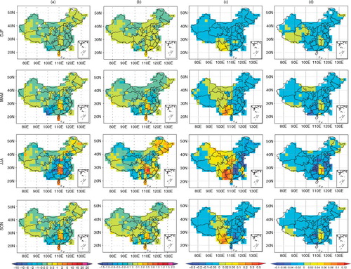
Figure 3a shows the distributions of simulated changes in seasonal mean isoprene emission from the late 1980s to the mid-2000s with the changes in both meteorological parameters and land cover (CTRL_2000s minus CTRL_1980s). Simulated changes in isoprene emission are small in December–January–February (DJF). Large increases in isoprene emissions of about 2–10×10⁶ kg C month⁻¹ (or 60–120% relative to CTRL_1980s) are found in March–April–May (MAM) over SE, especially in the middle and lower reaches of the Yangtze River, as a result of the relatively higher temperatures in the mid-2000s. The most significant absolute changes in isoprene emissions are found in June–July–August (JJA); relative to the late 1980s, isoprene emissions in the mid-2000s are simulated to increase largely by 10–25×10⁶ kg C month⁻¹ (30–90%) in the middleand lower reaches of the Yangtze River and by 5–10×10⁶ kg C month⁻¹ (20–80%) over NE, but to decrease by 1–5×10⁶ kg C month⁻¹ (10–40%) along the southeast coast of China, in Yunnan province in SW, and in Henan province in NE. Isoprene emissions in September–October–November (SON) are estimated to have large increases of 1–2×10⁶ kg C month⁻¹ (50–120%) in most places of NE and of 2–5×10⁶ kg C month⁻¹ (20–70%) over SE because of higher temperatures and the increased coverage of forests in those regions in the mid-2000s. The distributions of simulated changes in seasonal mean monoterpene emissions are shown in Fig. 3b. The changes in monoterpene emissions due to the changes in both land cover and meteorology from the late 1980s to the mid-2000s are generally one order of magnitude smaller than those in isoprene emissions, but the distribution of changes in monoterpene emissions is similar to that of isoprene in each of the four seasons.

Fig. 3 Simulated seasonal mean changes from the late 1980s to the mid-2000s as a result of changes in both land cover and meteorological parameters (CTRL_2000s minus CTRL_1980s): (a) isoprene emissions (unit: 10⁶ kg C month⁻¹), (b) monoterpene emissions (unit: 10⁶ kg C month⁻¹), (c) surface-layer O₃ (unit: ppbv), and (d) SOA concentrations (unit: µg m⁻³).

Simulated changes in annual BVOC emissions in different regions are summarised in Table 3. From the late 1980s to the mid-2000s, the annual isoprene emissions exhibited increases in all regions as a result of the changes in meteorology and land cover; isoprene emissions in regions of SE, SW, and NE are simulated to increase by 13.1, 6.4, and 23.0%, respectively, but the absolute changes in isoprene emissions over the NW and PT regions are found to be very small. Simulated annual monoterpene emissions exhibited increases of 7.4% in SE and 8.7% in NE whereas a decrease by 10.8% in NW over the time period.

4.2. The impact of changes in land cover and land use on biogenic emissions

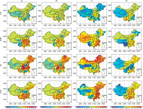
As a result of the changes in LCLU alone (SENS_LCLU minus CTRL_1980s), annual emissions of isoprene, monoterpenes and other VOC in China are simulated to change by −3.5, −3.1 and −2.3%, respectively (Table 3). The seasonal mean isoprene emissions are simulated to decrease by 0.5–1.0×10⁶ kg C month⁻¹ (or 5–30%) in many places of SE, SW and NW China, with maximum decreases of 2–5×10⁶ kg C month⁻¹ (10–40%) in JJA (Fig. 4a). The decreases in isoprene emissions in SE and SW regions were caused by the reductions in the coverage of tropical forests such as Elaeis guineensis, Cyclobalanopsis glauca, Eucalyptus globulus, Ficus auriculata Lour, Flueggea virosa, which were replaced by shrubs and grass (Fig. 2) that emitted less isoprene than those forest species (Kesselmeier and Staudt, 1999; Klinger et al., 2002; Guenther et al., 2006; Li et al., 2013). The reduction of annual isoprene emission in NW resulted from the reduced areas of grassland and the desertification process over that region (Fig. 2). Isoprene emissions in NE and in Hunan and Hubei provinces in SE region are simulated to increase by 2–10×10⁶ kg C month⁻¹ (10–20%) in JJA and by 1–2×10⁶ kg C month⁻¹ (10%) in other seasons (Fig. 4a), as a result of the increases in the coverage of temperate forests and crops. Klinger et al. (2002) reported that plant species such as Populus, Quercus mongolica, Quercus liaotungensis, Salix viminalis, Robinia pseudoacacia, Maackia amurensis distributed in these regions were of high isoprene emission capacity. With changes in LCLU alone, emissions of monoterpenes are simulated to decrease by 0.2–0.8×10⁶ kg C month⁻¹ (10–30%) in SW and NW China owing to the reductions in vegetation cover in western China (e.g. Hevea brasiliensis, Pometia tomentosa, Pinus armandi), but to increase by up to 0.5–1.2×10⁶ kg C month⁻¹ (10–20%) in JJA in SE and NE China (Fig. 4b) as a result of the increases in coverage of temperate forests (e.g. Betula platyphylla, Pinus, Abies, Picea, Cupressus) and shrub (e.g. Ledum palustre, Alchornea trewioides) (Klinger et al., 2002; Li et al., 2013).

Fig. 4 Simulated seasonal mean changes from the late 1980s to the mid-2000s as a result of the changes in land cover alone (SENS_LCLU minus CTRL_1980s): (a) isoprene emissions (unit: 10⁶ kg C month⁻¹), (b) monoterpene emissions (unit: 10⁶ kg C month⁻¹), (c) surface-layer O₃ (unit: ppbv), and (d) SOA concentrations (unit: µg m⁻³). Note that the magnitudes of changes in O₃ and SOA are different from those in Fig. 3.

From the late 1980s to the mid-2000s, the annual isoprene emissions exhibited decreases in most regions as a result of the changes in LCLU alone (Table 3). Isoprene emission in SW showed the largest change of −12.5% and the absolute decreases in isoprene emissions in other regions are at least one order of magnitude smaller than the change in SW. Simulated annual monoterpene emissions exhibited changes of −6.2% in SW, −2.1% in NE, and −14.9% in NW.

4.3. The impact of changes in meteorological conditions on biogenic emissions

As a result of the changes in meteorological conditions alone (SENS-MET minus CTRL_1980s), annual emissions of isoprene, monoterpenes, and other VOCs over China are simulated to change by +17.0, +7.9 and +13.3%, respectively. For the isoprene emissions, the increases of 0.5×10⁶ kg C month⁻¹ (or 30–120%) occurred in most places of NE and NW in DJF. Large increases in isoprene emission were over a large fraction of SE in MAM and SON, with the maximum increases in the range of 2–10×10⁶ kg C month⁻¹ (60–100%). Isoprene emissions in NE and the middle and lower reaches of the Yangtze River in SE showed largest increases of 10–25×10⁶ kg C month⁻¹ (60–90%) in JJA (Fig. 5a). As shown in Fig. 5b, changes in monoterpene emissions were within the range of −0.8 to +2.0×10⁶ kg C month⁻¹ (–10 to +60%) and exhibited similar spatial patterns in all seasons as those of changes in isoprene emissions.

From the late 1980s to the mid-2000s, the changes in meteorological fields generally had larger impacts on annual isoprene and monoterpene emissions than the changes in LCLU alone (Table 3), except that in the SW and NW regions the percentage changes in isoprene and monoterpene emissions resulted from the changes in LCLU were comparable to those resulted from changes in meteorological parameters, indicating that LCLU changes played an important role in influencing biogenic emissions on decadal time scale. While the changes in meteorological parameters from the late 1980s to the mid-2000s led to increases in annual BVOC emissions, the LCLU changes over the same time period induced decreases in annual BVOC emissions.

5. Simulated changes in concentrations of surface-layer O₃ and SOA

The performance of the GEOS-Chem model in simulating the temporal and spatial distribution of O₃ in China has been evaluated in previous studies for China (Wang et al., 2008b, 2011b; Jeong and Park, 2013; Lou et al., 2014). They have demonstrated that the GEOS-Chem model captures well the magnitude and seasonal variation of surface-layer O₃ concentrations in China. The simulated changes in seasonal mean surface-layer O₃ concentrations from the late 1980s to the mid-2000s due to the combined effects of changes in meteorological fields and LCLU are shown in Fig. 3c (CTRL_2000s minus CTRL_1980s). With anthropogenic emissions fixed at year 2005 levels, increases in O₃ concentration of 0.5–2.0 ppbv are simulated in DJF in the middle and lower reaches of the Yangtze River in SE and in the Huabei plain in NE. These increases in O₃ over SE and NE in winter were caused by the increases in temperature and enhanced biogenic emissions in those VOCs-limited regions (Chou et al., 2009; Tang et al., 2012). In MAM, with the combined effects of changes in meteorological parameters and LCLU, O₃ concentrations increased by 0.5–4 ppbv in a large fraction of China, and the concentrations in SW decreased by 0.5–3 ppbv. In JJA and SON, concentrations of O₃ in NE, SE and SW China exhibited increases of about 1–6 ppbv, whereas those in the plateau region decreased by 1–4 ppbv. Note that, in JJA, simulated O₃ decreased from the late 1980s to the mid-2000s in central China (centred around 30°N, 105°E) where simulated increases in isoprene and monoterpene emissions are large. These decreases in O₃ can be explained by the VOC/NO_x ratio. Because central China is NO_x-limited in summer, increases in isoprene emissions reduce O₃ concentration by sequestering NO_x as isoprene nitrates (Fiore et al., 2005).

Comparisons of Fig. 4c (simulated changes in O₃ as a results of the changes in LCLU alone, SENS_LCLU minus CTRL_1980s) and Fig. 5c (simulated changes in O₃ as a results of the changes in meteorological parameters alone, SENS_MET minus CTRL_1980s) indicate that the changes in surface-layer O₃ concentrations were mainly driven by the changes in meteorological fields and the associated changes in BVOC emissions from the late 1980s to the mid-2000s. The changes in O₃ concentrations from the late 1980s to the mid-2000s resulted from the decadal changes in LCLU alone were within ±0.5 ppbv over China (Fig. 5c).

Fig. 5 Simulated seasonal mean changes from the late 1980s to the mid-2000s a result of changes in meteorological parameters alone (SENS_MET minus CTRL_1980s): (a) isoprene emissions (unit: 10⁶ kg C month⁻¹), (b) monoterpene emissions (unit: 10⁶ kg C month⁻¹), (c) surface-layer O₃ (unit: ppbv), and (d) SOA concentrations (unit: µg m⁻³).

The simulated changes in SOA concentrations from the late 1980s to the mid-2000s are shown in Fig. 3d. With anthropogenic emissions fixed at the year 2005 values, the changes in SOA concentrations from the late 1980s to the mid-2000s ranged from −0.4 to +0.6 µg m⁻³, as a result of changes in both meteorological parameters and LCLU. Simulated SOA concentrations decreased from the late 1980s to the mid-2000s in central China (centred around 30°N, 105°E), although simulated isoprene and monoterpene emissions increased in this region. These decreases in SOA can be explained by the changes in meteorological conditions in summer. While the increases in temperature enhance biogenic emissions, higher temperatures shift the gas-particle partitioning of volatile oxidation products toward the gas-phase (Liao et al., 2006). The decadal changes in LCLU alone led to prevailing decreases in surface-layer SOA concentrations over China (Fig. 5c), with the maximum reductions in SOA concentrations by 0.1 µg m⁻³.

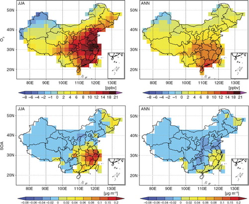
Fig. 6 Simulated changes in summer (JJA) and annual mean surface-layer concentrations of O₃ and SOA as a result of changes in anthropogenic emissions over 1985–2005 (CTRL_2000s minus SENS_ANTH). Unit is ppbv for O₃ and µg m⁻³ for SOA.

6. Comparison with the impact of changes in anthropogenic emissions

We also perform a sensitivity simulation SENS_ANTH (described in Section 2.4) to quantify the impact of changes in anthropogenic emissions from 1985 to 2005 on concentrations of O₃ and SOA with the meteorological field and vegetation parameters fixed at year 2005 values. Relative to year 1985, anthropogenic emissions of NO_x, CO, and non-methane hydrocarbons over China in year 2005 increased by 117, 150, and 89%, respectively. As a result, surface-layer O₃ concentrations is enhanced in most places of China(Fig. 6). Simulated maximum increases in JJA O₃ reached 21 ppbv in eastern China. Such changes in JJA surface-layer O₃ concentration owing to the changes in anthropogenic emissions between 1985 and 2005 were larger than the changes simulated with combined changes in meteorological conditions and LCLU (Fig. 3c). While the changes in anthropogenic emissions generally increased O₃ concentrations in China, the changes in meteorological parameters and LCLU led to reductions in O₃ concentrations in some places (e.g. central China). The effect of changes in meteorological and LCLU offset the increases caused by anthropogenic emissions by about 5–10% in central China.

The changes in anthropogenic emissions from 1985 to 2005 are simulated to increase JJA surface-layer SOA concentrations by as much as 0.2 µg m⁻³ in southeastern China (Fig. 6). Compared to the changes in JJA SOA concentration owing to the combined effect of meteorological and LCLU changes (Fig. 3d), the magnitude of changes in JJA SOA concentrations due to the changes in anthropogenic emissions was smaller in places of SE China (regions around 30°N) but in the opposite sign. In the coastal regions of SE China, the effects of changes in anthropogenic emissions were comparable with changes in meteorological conditions and LCLU.

7. Conclusions and discussions

We use the biogenic emission module MEGAN embedded within the global chemical transport model GEOS-Chem to estimate the changes in BVOC emissions and hence in surface-layer concentrations of O₃ and SOA over China from the late 1980s to the mid-2000s. LCLU datasets in China in this time period are based on satellite retrieval and land use survey. From the late 1980s to the mid-2000s, total area of vegetation coverage in China decreased by 4%. The fractions of land covered by forests exhibited increases of 10–30 and 5–15%, respectively, in SE and NE China and decreases of 15–35% in SW China. The fractions of cropland decreased in most regions except for in the farming–pastoral zone in northern China where cropland increased by 5–20%. The factions of grassland in northern China showed large reductions of 5–30%.

From the late 1980s to the mid-2000s, the annual biogenic emissions of isoprene, monoterpenes, and OVOCs in China are simulated to increase by +13.1, +4.6, and +10.8%, respectively, as changes in both meteorological fields and LCLU are considered. The changes in meteorological parameters are simulated to have a larger effect on BVOC emissions than the changes in LCLU alone. As a result of the changes in meteorological fields (LCLU) alone, the annual total BVOC emission in china is simulated to change by +15.2% (−3.3%) from the late 1980s to the mid-2000s. Note that locally, in the SW and NW regions, the percentage changes in isoprene and monoterpene emissions resulted from the changes in LCLU were comparable to those resulting from changes in meteorological parameters.

With anthropogenic emissions of O₃ precursors, aerosol precursors, and aerosols fixed at year 2005 levels, the changes in meteorological parameters and in LCLU from the late 1980s to the mid-2000s are simulated to change the seasonal mean surface-layer O₃ concentrations by −4 to +6 ppbv and to change the seasonal mean surface-layer SOA concentrations by −0.4 to +0.6 µg m⁻³ over China. We also perform a sensitivity simulation SENS_ANTH to compare the impacts of changes in anthropogenic emissions on concentrations of O₃ and SOA with those of the changes in meteorological parameters and land cover. Results show that changes in anthropogenic emissions over 1985–2005 alone enhanced JJA surface-layer O₃ concentrations by 10–21 ppbv and increased JJA surface-layer SOA concentrations by as much as 0.2 µg m⁻³ in southeastern China. Compare with the impact of anthropogenic emissions, the changes induced by meteorological and vegetation changes are significant, considering that the present-day seasonal mean O₃ concentrations in China are in the range of 20–60 ppbv (Lou et al., 2014; Yang et al., 2014) and that the simulated present-day seasonal mean SOA concentrations in China have maximum concentrations of about 2.0–2.5 µg m⁻³ (Fu and Liao, 2012; Fu et al., 2012). The changes in meteorological fields influence O₃ and SOA concentrations in two ways. First, the emissions of BVOCs vary with meteorological fields. Second, the changes in meteorological parameters influence chemical reactions, transport, and deposition of O₃ and SOA.

There are some sources of uncertainties in our simulations that need to be improved in future studies. The emission factor is one of the key sources of uncertainties for estimating biogenic emissions. We assume that the vegetation composition (in terms of biogenic emission rates) for each PFT remain unchanged from the late 1980s to the mid-2000s since the MEGAN scheme resolves the PFTs but not detailed plant species. A few previous studies have tried to use plant species level emission factors from local measurements for estimating biogenic emissions in China (Klinger et al., 2002; Zhao et al., 2004; Tsui et al., 2009; Wang et al., 2011a). Wang et al. (2011a) assessed the impacts of PFTs, surface meteorological variables, and EFs on BVOC emissions in PRD region. They found that the total isoprene emission obtained using the globally averaged EFs was 2.5 times higher than that estimated using regional EFs, whereas the total emission of monoterpenes or sesquiterpene was lower by about 42% as emission estimated using the globally averaged EFs was compared with that estimated using the local EFs. Guenther et al. (2012) reported that the uncertainties associated with the global annual emission are about a factor of two for isoprene and about a factor of three or higher for monoterpenes and other compounds. Compared to the EFs in Guenther et al. (2012), the isoprene EFs in our study are lower for broadleaf trees and shrubs (the PFTs with large isoprene emissions) whereas higher for temperate evergreen needleleaf trees and crops. As a result, the estimated isoprene emissions in our study are likely lower than those estimated for China in Guenther et al. (2012). However, the distributions of PFTs in our study are different from those in Guenther et al. (2012), so it's hard for us to quantify the differences in estimated BVOC emissions between our work and other studies on the basis of the differences in EFs alone. Another source of uncertainties arise from our assumption about LAI; because LAI datasets from the MODIS product are not available for the late 1980s, the averaged LAI from MODIS over 2001–2006 are used in our simulations. Hence, more measurements are needed to reduce uncertainties in estimated biogenic emissions.

Furthermore, the impacts of land cover change on dry deposition of O₃ and SOA and on soil emissions of nitrogen oxide (NO_x) are not considered here, which have been shown to be important in Wu et al. (2012) and Tai et al. (2013). Finally, the GEOS-Chem model underestimates SOA in China (Fu et al., 2008, 2012), which is undergoing continuing improvement based on recent laboratory chamber studies. These issues suggest avenues for improvement in our future research.

Acknowledgements

This work was supported by the National Basic Research Program of China (973 program, Grant No. 2014CB441202), the Chinese Academy of Sciences Strategic Priority Research Program (Grant No. XDA05100503), the National Natural Science Foundation of China under grants 41475137 and 41321064, as well as the National High Technology Research and Development Program of China (Grant No. 2013AA122002). We acknowledge the MODIS LAI product provided by Land Processes Distributed Active Archive Center (LP DAAC).

References

- Alexander B. , Park R. J. , Jacob D. J. , Li Q. B. , Yantosca R. M. , co-authors . Sulfate formation in sea-salt aerosols: constraints from oxygen isotopes. J. Geophys. Res. 2005; 110: 10307.
- Arneth A. , Schurgers G. , Lathiere J. , Duhl T. , Beerling D. J. , co-authors . Global terrestrial isoprene emission models: sensitivity to variability in climate and vegetation. Atmos. Chem. Phys. 2011; 11: 8037–8052.
- Bai J. H. , Baker B. , Liang B. S. , Greenberg J. , Guenther A . Isoprene and monoterpene emissions from an inner Mongolia grassland. Atmos. Environ. 2006; 40: 5753–5758.
- Barkley M. P. , Palmer P. I. , Ganzeveld L. , Arneth A. , Hagberg D. , co-authors . Can a “state of the art” chemistry transport model simulate Amazonian tropospheric chemistry?. J. Geophys. Res. 2011; 116: 16302.
- Bey I. , Jacob D. J. , Yantosca R. M. , Logan J. A. , Field B. D. , co-authors . Global modeling of tropospheric chemistry with assimilated meteorology: model description and evaluation. J. Geophys. Res. 2001; 106: 23073–23095.
- Carslaw K. S. , Boucher O. , Spracklen D. V. , Mann G. W. , Rae J. G. L. , co-authors . A review of natural aerosol interactions and feedbacks within the Earth system. Atmos. Chem. Phys. 2010; 10: 1701–1737.
- Chen Y. , Tang H . Desertification in north China: background, anthropogenic impacts and failures in combating it. Land Degrad. Dev. 2005; 16: 367–376.
- Chou C. C. K. , Tsai C.-Y. , Shiu C.-J. , Liu S. C. , Zhu T . Measurement of NOy during Campaign of Air Quality Research in Beijing 2006 (CAREBeijing-2006): implications for the ozone production efficiency of NOx. J. Geophys. Res. 2009; 114: 00G01.
- CNIS. Names and Codes for Climate Regionalization in China-Climatic Zones and Climatic Regions (GB/T 17297-1998). 1998. Standardization Administration of China, Beijing. (in Chinese)..
- Cramer W. , Bondeau A. , Woodward F. I. , Prentice I. C. , Betts R. A. , co-authors . Global response of terrestrial ecosystem structure and function to CO2 and climate change: results from six dynamic global vegetation models. Global Change Biol. 2001; 7: 357–373.
- Fairlie T. D. , Jacob D. J. , Park R. J . The impact of transpacific transport of mineral dust in the United States. Atmos. Environ. 2007; 41: 1251–1266.
- Fiore A. M. , Horowitz L. W. , Purves D. W. , Levy H. , Evans M. J. , co-authors . Evaluating the contribution of changes in isoprene emissions to surface ozone trends over the eastern United States. J. Geophys. Res. 2005; 110: D12303.
- Fu T. M. , Cao J. J. , Zhang X. Y. , Lee S. C. , Zhang Q. , co-authors . Carbonaceous aerosols in China: top-down constraints on primary sources and estimation of secondary contribution. Atmos. Chem. Phys. 2012; 12: 2725–2746.
- Fu T. M. , Jacob D. J. , Wittrock F. , Burrows J. P. , Vrekoussis M. , Henze D. K . Global budgets of atmospheric glyoxal and methylglyoxal, and implications for formation of secondary organic aerosols. J. Geophys. Res. 2008; 113: D15303.
- Fu Y. , Liao H . Simulation of the interannual variations of biogenic emissions of volatile organic compounds in China: impacts on tropospheric ozone and secondary organic aerosol. Atmos. Environ. 2012; 59: 170–185.
- Ganzeveld L. , Bouwman L. , Stehfest E. , van Vuuren D. P. , Eickhout B. , co-authors . Impact of future land use and land cover changes on atmospheric chemistry-climate interactions. J. Geophys. Res. 2010; 115: 23301.
- Guenther A. , Hewitt C. N. , Erickson D. , Fall R. , Geron C. , co-authors . A global model of natural volatile organic compound emissions. J. Geophys. Res. 1995; 100: 8873–8892.
- Guenther A. , Karl T. , Harley P. , Wiedinmyer C. , Palmer P. I. , co-authors . Estimates of global terrestrial isoprene emissions using MEGAN (Model of Emissions of Gases and Aerosols from Nature). Atmos. Chem. Phys. 2006; 6: 3181–3210.
- Guenther A. B. , Jiang X. , Heald C. L. , Sakulyanontvittaya T. , Duhl T. , co-authors . The Model of Emissions of Gases and Aerosols from Nature version 2.1 (MEGAN2.1): an extended and updated framework for modeling biogenic emissions. Geosci. Model Dev. 2012; 5: 1471–1492.
- Gulden L. E. , Yang Z. L. , Niu G. Y . Sensitivity of biogenic emissions simulated by a land-surface model to land-cover representations. Atmos. Environ. 2008; 42: 4185–4197.
- Henze D. K. , Seinfeld J. H . Global secondary organic aerosol from isoprene oxidation. Geophys. Res. Lett. 2006; 33: 09812.
- Henze D. K. , Seinfeld J. H. , Ng N. L. , Kroll J. H. , Fu T. M. , co-authors . Global modeling of secondary organic aerosol formation from aromatic hydrocarbons: high- vs. low-yield pathways. Atmos. Chem. Phys. 2008; 8: 2405–2420.
- Hurtt G. C. , Chini L. P. , Frolking S. , Betts R. A. , Feddema J. , co-authors . Harmonization of land-use scenarios for the period 1500–2100: 600 years of global gridded annual land-use transitions, wood harvest, and resulting secondary lands. Clim. Change. 2011; 109: 117–161.
- Hou X. Y . Vegetation Atlas of China (1:1000000). 2001; Beijing: Science Press. (in Chinese).
- IPCC. Solomon S. , co-editors . Contribution of working group I to the fourth assessment report of the intergovernmental panel on climate change. Climate Change 2007: The Physical Science Basis. 2007; Cambridge,, UK: Cambridge University Press. 1–996.
- Jeong J. I. , Park R. J . Effects of the meteorological variability on regional air quality in East Asia. Atmos. Environ. 2013; 69: 46–55.
- Kesselmeier J. , Staudt M . Biogenic volatile organic compounds (VOC): an overview on emission, physiology and ecology. J. Atmos. Chem. 1999; 33: 23–88.
- Klinger L. F. , Li Q. J. , Guenther A. B. , Greenberg J. P. , Baker B. , co-authors . Assessment of volatile organic compound emissions from ecosystems of China. J. Geophys. Res. 2002; 107: 4603.
- Lathiere J. , Hauglustaine D. A. , Friend A. D. , De Noblet-Ducoudre N. , Viovy N. , co-authors . Impact of climate variability and land use changes on global biogenic volatile organic compound emissions. Atmos. Chem. Phys. 2006; 6: 2129–2146.
- Lathiere J. , Hewitt C. N. , Beerling D. J . Sensitivity of isoprene emissions from the terrestrial biosphere to 20th century changes in atmospheric CO2 concentration, climate, and land use. Global Biogeochem. Cy. 2010; 24: 1004.
- Leung D. Y. C. , Wong P. , Cheung B. K. H. , Guenther A . Improved land cover and emission factors for modeling biogenic volatile organic compounds emissions from Hong Kong. Atmos. Environ. 2010; 44: 1456–1468.
- Levis S. , Wiedinmyer C. , Bonan G. B. , Guenther A . Simulating biogenic volatile organic compound emissions in the Community Climate System Model. J. Geophys. Res. 2003; 108(D21): 4659.
- Li L. Y. , Chen Y. , Xie S. D . Spatio-temporal variation of biogenic volatile organic compounds emissions in China. Environ. Pollut. 2013; 182: 157–168.
- Liao H. , Chen W. T. , Seinfeld J. H . Role of climate change in global predictions of future tropospheric ozone and aerosols. J. Geophys. Res. 2006; 111: 12304.
- Liao H. , Henze D. K. , Seinfeld J. H. , Wu S. L. , Mickley L. J . Biogenic secondary organic aerosol over the United States: comparison of climatological simulations with observations. J. Geophys. Res. 2007; 112: 06201.
- Liu J . Macro-scale survey and dynamic study of natural resources and environment of Chinese by remote sensing. 1996; Chinese Science and Technology Press, Beijing.
- Liu J. , Buhe A . Study on spatial-temporal feature of modern land -use change in China: using remote sensing techniques. Quaternary Sci. 2000; 20: 229–239.
- Liu J. , Liu M. , Deng X. , Zhuang D. , Zhang Z. , co-authors . The land use and land cover change database and its relative studies in China. J. Geophys. Res. 2002; 12: 275–282.
- Liu J. , Liu M. , Tian H. , Zhuang D. , Zhang Z. , co-authors . Spatial and temporal patterns of China's cropland during 1990–2000: an analysis based on Landsat TM data. Rem. Sens. Environ. 2005b; 98: 442–456.
- Liu J. , Tian H. , Liu M. , Zhuang D. , Melillo J. M. , co-authors . China's changing landscape during the 1990s: large-scale land transformations estimated with satellite data. Geophys. Res. Lett. 2005a; 32: L02405.
- Liu J. , Zhang Z. , Xu X. , Kuang W. , Zhou W. , co-authors . Spatial patterns and driving forces of land use change in China during the early 21st century. J. Geogr. Sci. 2010; 20: 483–494.
- Liu J. , Zhuang D. F. , Luo D. , Xiao X . Land-cover classification of China: integrated analysis of AVHRR imagery and geophysical data. Int. J. Rem. Sens. 2003; 24: 2485–2500.
- Liu M. , Tang X. , Liu J. , Zhuang D . Research on scaling effect based on 1 km grid cell data. J. Rem. Sens. 2001; 5: 10.
- Liu M. L. , Tian H. Q . China's land cover and land use change from 1700 to 2005: estimations from high-resolution satellite data and historical archives. Global Biogeochem. Cy. 2010; 24: GB3003.
- Liu R. , Liang S. , Liu J. , Zhuang D . Continuous tree distribution in China: a comparison of two estimates from Moderate-Resolution Imaging Spectroradiometer and Landsat data. J. Geophys. Res. 2006; 111: D08101.
- Lou S. , Liao H. , Zhu B . Impacts of aerosols on surface-layer ozone concentrations in China through heterogeneous reactions and changes in photolysis rates. Atmos. Environ. 2014; 85: 123–138.
- Müller J. F. , Stavrakou T. , Wallens S. , De Smedt I. , Van Roozendael M. , co-authors . Global isoprene emissions estimated using MEGAN, ECMWF analyses and a detailed canopy environment model. Atmos. Chem. Phys. 2008; 1329–1341. 8 .
- Olivier J. G. J. , Berdowski J. J. M . Berdowski J. , Guicherit R. , Heij B. J . Global emissions sources and sinks. The Climate System. 2001; Lisse, The Netherlands: A. A. Balkema Publishers/Swets & Zeitlinger Publishers. 33–78.
- Olson J . World Ecosystems (WE1.4): digital raster data on a 10 minute geographic 1080×2160 grid. Global Ecosystems Database, Version 1.0: Disc A. 1992; edited by NOAA National Geophysical Data Center, Boulder, Colorado.
- Park R. J. , Jacob D. J. , Chin M. , Martin R. V . Sources of carbonaceous aerosols over the United States and implications for natural visibility. J. Geophys. Res. 2003; 108: 4355.
- Park R. J. , Jacob D. J. , Field B. D. , Yantosca R. M. , Chin M . Natural and transboundary pollution influences on sulfate–nitrate–ammonium aerosols in the United States: implications for policy. J. Geophys. Res. 2004; 109: D15204.
- Piccot S. D. , Watson J. J. , Jones J. W . A global inventory of volatile organic compound emissions from anthropogenic sources. J. Geophys. Res. 1992; 97: 9897–9912.
- Qiu X . Lin X. , co-editors . Chapter 11: General survey of cities. China Statistical Yearbook 2006. 2006; National Bureau of Statistics of China, China: China Statistics Press. 11–15.
- Sanderson M. G. , Jones C. D. , Collins W. J. , Johnson C. E. , Derwent R. G . Effect of climate change on isoprene emissions and surface ozone levels. Geophys. Res. Lett. 2003; 30(18): 1936.
- Situ S. , Guenther A. , Wang X. , Jiang X. , Turnipseed A. , co-authors . Impacts of seasonal and regional variability in biogenic VOC emissions on surface ozone in the Pearl River delta region, China. Atmos. Chem. Phys. 2013; 13: 11803–11817.
- Smiatek G. , Steinbrecher R. , Koble R. , Seufert G. , Theloke J. , co-authors . Intra- and inter-annual variability of VOC emissions from natural and semi-natural vegetation in Europe and neighbouring countries. Atmos. Environ. 2009; 43: 1380–1391.
- Stavrakou T. , Müller J. F. , Bauwens M. , De Smedt I. , Van Roozendael M. , co-authors . Isoprene emissions over Asia 1979–2012: impact of climate and land-use changes. Atmos. Chem. Phys. 2014; 14: 4587–4605.
- Streets D. G. , Bond T. C. , Carmichael G. R. , Fernandes S. D. , Fu Q. , co-authors . An inventory of gaseous and primary aerosol emissions in Asia in the year 2000. J. Geophys. Res. 2003; 108: 21.
- Streets D. G. , Zhang Q. , Wang L. , He K. , Hao J. , co-authors . Revisiting China's CO emissions after the transport and chemical evolution over the Pacific (TRACE-P) mission: synthesis of inventories, atmospheric modeling, and observations. J. Geophys. Res. 2006; 111: D14306.
- Tai A. P. K. , Mickley L. J. , Heald C. L. , Wu S . Effect of CO2 inhibition on biogenic isoprene emission: implications for air quality under 2000 to 2050 changes in climate, vegetation and land use. Geophys. Res. Lett. 2013; 40: 3479–3483.
- Tang G. , Wang Y. , Li X. , Ji D. , Hsu S. , co-authors . Spatial-temporal variations in surface ozone in Northern China as observed during 2009–2010 and possible implications for future air quality control strategies. Atmos. Chem. Phys. 2012; 12: 2757–2776.
- Tie X. , Li G. , Ying Z. , Guenther A. , Madronich S . Biogenic emissions of isoprenoids and NO in China and comparison to anthropogenic emissions. Sci. Total Environ. 2006; 371: 238–251.
- Tsui J. K. Y. , Guenther A. , Yip W. K. , Chen F . A biogenic volatile organic compound emission inventory for Hong Kong. Atmospheric Environment. 2009; 43: 6442–6448.
- Wang X. , Chen F. , Hasi E. , Li J . Desertification in China: an assessment. Earth Sci. Rev. 2008a; 88: 188–206.
- Wang X. M. , Situ S. P. , Guenther A. , Chen F. , Wu Z. Y. , co-authors . Spatiotemporal variability of biogenic terpenoid emissions in Pearl River Delta, China, with high-resolution land-cover and meteorological data. Tellus B. 2011a; 63: 241–254.
- Wang Y. , McElroy M. B. , Munger J. W. , Hao J. , Ma H. , co-authors . Variations of O3 and CO in summertime at a rural site near Beijing. Atmos. Chem. Phys. 2008b; 8: 6355–6363.
- Wang Y. , Zhang Y. , Hao J. , Luo M . Seasonal and spatial variability of surface ozone over China: contributions from background and domestic pollution. Atmos. Chem. Phys. 2011b; 11: 3511–3525.
- Willson A . Forest conversion and land use change in rural northwest Yunnan, China. Mt. Res. Dev. 2006; 26: 227–236.
- Wu S. , Mickley L. J. , Kaplan J. O. , Jacob D. J . Impacts of changes in land use and land cover on atmospheric chemistry and air quality over the 21st century. Atmos. Chem. Phys. 2012; 12: 1597–1609.
- Wu W. , Shibasaki R. , Yang P. , Ongaro L. , Zhou Q. , co-authors . Validation and comparison of 1 km global land cover products in China. Int. J. Rem. Sens. 2008; 29: 3769–3785.
- Yang Y. , Liao H. , Li J . Impacts of the East Asian summer monsoon on interannual variations of summertime surface-layer ozone concentrations over China. Atmos. Chem. Phys. 2014; 14: 3269–3300.
- Zemankova K. , Brechler J . Emissions of biogenic VOC from forest ecosystems in central Europe: estimation and comparison with anthropogenic emission inventory. Environ. Pollut. 2010; 158: 462–469.
- Zhang X. S . Vegetation map of the People's Republic of China (1:1000000). 2007; Beijing: Geological Publishing House. (in Chinese).
- Zhao J. , Bai Y. , Wang Z. , Zhang S . Studies on the emission rates of plants VOCs in China. China Environmental Science. 2004; 24: 654–657. (in Chinese).
- Zhao J. , Zheng Z. , Yu Y. , Zhong L . Temporal, spatial characteristics and uncertainty of biogenic VOC emissions in the Pearl River Delta region, China. Atmos. Environ. 2010; 44: 1960–1969.