One-year measurement of size-resolved particle fluxes in an urban area

Abstract

Size-resolved particle flux measurements were carried out in an urban area from April 2012 to April 2013. Together with a standard eddy covariance system, two fast optical particle counters have been employed on a 65-meter-high tower in Münster, Germany. Particle number fluxes were directly calculated for particles with diameters from 0.06 to 10 µm within 16 individual size-bins. Whereas particle number concentrations show a distinct yearly pattern with maxima in winter and minima in summer, the flux time series is more multifaceted. Average daily maxima of 3.0e+07 particles m⁻² s⁻¹ occurred during winter while minima of 2.0e+06 particles m⁻² s⁻¹ were observed in fall. The size-resolved measurements revealed that during spring and summer a considerable number of accumulation mode particles deposits while a simultaneous net particle emission occurred, which is mostly driven by particles smaller than 0.12 µm. These bi-directional fluxes lead to a net mass deposition of up to 13.5 µg m⁻² d⁻¹. The tipping-point between the emission and deposition lay between 0.16 and 0.19 µm. In a comprehensive analysis of the flux and concentration time series, the degree of atmospheric stability, the seasons, and the type of source region have been identified as key influences for particle fluxes. Different responses between particle fluxes and concentrations have been found along these drivers.

• eddy covariance
• aerosol particle
• size segregated
• flux
• urban

1. Introduction

Urban areas exhibit a variety of well-known particle sources, such as products from traffic exhaust, re-suspension of road dust, emission from industrial combustion, and, not least, domestic emissions from heating, cooking and wood burning. The exchange of aerosol particles between a city and the atmosphere is of importance since, in contrast to highly reactive trace gases, particles are relatively long-lived substances and can be transported over long distances. In the past, different methodologies (reviewed in, e.g. Gallagher et al., 1997b; Nicholson, 1988; Pryor et al., 2008) were used to study the transfer of particles to different surfaces (dry deposition). With an increasing development of fast particle sizing and detection instrumentation over the last 15 yr it became possible to apply the ‘Eddy Covariance’ (EC) technique to particle number concentrations. To the current date, EC is the most direct method to estimate the turbulent vertical exchange of a scalar above a surface. First particle EC-measurements were conducted in the 1980s (e.g. Hicks et al., 1982; Katen and Hubbe, 1985), but didn't become popular before the late 1990s after publications from Gallagher et al. (1997) and Buzorius et al. (1998). While these early studies focused on natural environments, the first flux studies in an urban area were performed by Nemitz et al. (2000) and Dorsey et al. (2002). The authors found pronounced daily patterns of aerosol fluxes above Edinburgh (Scotland), with emissions that were correlated to traffic activity and the boundary layer stability. As a result, a first empirical equation was derived to parameterise aerosol concentrations determined by traffic flow rate and stability. In this course, Martin et al. (2009) summarised results from ultrafine particle flux measurement from four major European cities and present a parameterised model which predicts ultrafine particle fluxes based on traffic activity, sensible heat (SH) and friction velocity. Vogt et al. (2011a) developed a further parameterisation, which predicts sub-micrometre aerosol emissions from traffic sources as a function of the friction velocity and the CO₂ emission flux.

Besides these first flux studies, substantial research effort was spent on identifying urban particle size distributions and on characterising sampled urban aerosol in terms of its chemical composition and origin. It was found that physical properties, chemical reactivity, age and origin of urban particles vary notably as a function of particle size. Despite these previous findings, knowledge about size- and chemical-resolved fluxes and exchange velocities (which is the flux normalised by the respective particle number concentration) of particles is still lacking, as pointed out in the most recent review on particle atmosphere–surface exchange by Pryor et al. (2008). First approaches on chemical-resolved particle fluxes using aerosol mass spectroscopy (AMS) are described in Held et al. (2003), and a first application in an urban environment is presented in Nemitz et al. (2008), whereas Nemitz et al. (2000), Noone et al. (2003), Longley et al. (2004) and Schmidt and Klemm (2008) published first results on size-resolved particle fluxes and exchange velocities in urban areas. The authors commonly found that ultrafine particle fluxes govern total particle fluxes and show spatial and temporal variation which is closely linked to traffic activity, whereas accumulation mode particles (0.1–1 µm) proved to be less directly affected by urban sources and anthropogenic activities. On the other hand, super micrometre particles were found to be linked to high wind speeds, re-suspension and mechanical sources. Schmidt and Klemm (2008) found that particle number fluxes in the city of Münster Germany, generally decreased with particle diameter and inverted to negative fluxes and transfer velocities for accumulation mode particles larger than 0.32 µm. These bi-directional fluxes resulted in a net deposition of particle mass, while simultaneously particle number fluxes were strictly positive (emission). This seemingly contradictory observation was confirmed in a subsequent study with a much higher size resolution as presented in Deventer et al. (2013). The most recent reports on size-segregated particle flux measurements in urban areas are commonly campaign-based (Harrison et al., 2012; Deventer et al., 2013), whereas results from long term studies of size-resolved fluxes were only presented once for the city of Stockholm, Sweden, in Vogt et al. (2011b) and two times for bulk fluxes at the suburban SMEAR III site in Helsinki, Finland, by Järvi et al. (2009) and subsequently by Ripamonti et al. (2013). Therefore a size-resolved particle flux setup was employed in the city of Münster and operated for a sampling period of 1 yr. The aim was to detect seasonal variations of the highly resolved particles fluxes over this urban conglomeration in Central Europe.

2. Materials and methods

2.1. Study site and instrumentation

Measurements were made from April 2012 until April 2013 in the city of Münster (NW Germany, 51.9N, 7.6E, urban flux network: Mu06). Alongside traffic, industrial combustion, power generation, long range transport (e.g. of ammonium nitrate out of agricultural emissions), and sea salt emissions are well known particle sources for the study area (Gietl et al., 2008; Gietl and Klemm, 2009). Further, wood burning is a common practice during the winter season (BRMS.NRW, 2009).

For this study, we added the Passive Cavity Aerosol Spectrometer Probe (PCASP-X2, Droplet Measurement Technologies, Boulder, CO, USA) to the existing OPC (Ultra-High Sensitivity Aerosol Spectrometer, UHSAS) flux setup completed by a sonic anemometer and a fast CO₂/H₂O analyser as described in Deventer et al. (2013). Both OPCs combined detect particles with diameters from 0.55 up to 10 µm and classify them into 140 size channels. All sensor inlets were mounted 65 m above ground level (4.3 times the mean building height (z _h)=16.25 m). Air was aspirated through TYGON tubing of 2.7/2.5 m (UHSAS/PCASP-X2) length and 1/16 inch (about 1.6 mm) inner diameter with a sample flow rate of 0.83/0.1 cm³ s⁻¹, resulting in particle Reynolds numbers of 0.002<Re<0.02/0.004<Re<0.1 [eq. (4–1); Baron and Willeke, 2005]. The OPCs were placed perpendicularly to the sonic anemometer to ensure vertical alignment of the sampling lines with the exception of the one inlet bend (ca. 160°) to prevent direct rain entrainment. Additionally a small funnel of 1 cm diameter was used as a coating of the final part of the inlet line, to prevent the absorption of condensed water droplets.

Previous studied showed that the tower's height, structure and location are suitable for EC measurements with averaging intervals of 30 minutes and that the sampled air is representative for the urban area (Griessbaum and Schmidt, 2009; Dahlkötter et al., 2010; Deventer et al., 2013).

Because the measurement tower is located at the easterly border of the city, fluxes could be classified into two different flux source sectors: (1) an urban sector for wind directions between 180 and 360° and (2) a suburban sector (90–180°). Sector (1) covers the city centre with densely built up residential and central business areas, encircling highways, an inland harbour, the central train station and a few medium-sized industrial areas. Sector (2) contains residential areas with suburban structures, allotment garden grounds, agricultural areas and small forest patches. Note, that prevailing winds are S to W with a relative frequency of urban footprints of 70–80%. Besides the unequal wind direction distribution, the two sectors also differ in atmospheric conditions. The urban sector favours unstable to neutral (ζ≤0.01) conditions (67% relative frequency) with slightly but significantly (p<0.05, Kruskal–Wallis ANOVA) higher wind speeds (median=4.8 m s ⁻¹) and friction velocities (median=4.5 m s⁻¹), whereas the suburban sector tends toward more stable conditions (ζ>0.01, 59% relative frequency) with weaker wind speeds (median=4.2 m s⁻¹) and friction velocities (median=0.28 m s⁻¹), respectively. The wind direction distribution was fairly uniform throughout the measurement period and did not show significant seasonal changes.

2.2. EC data processing and flux calculation

Turbulent vertical particle number fluxes (F _N) were calculated as the covariance of instantaneous fluctuations of the vertical wind component (w′) and particle number concentrations (N′) for an averaging interval of 30 minutes:1

Particle mass fluxes (F _M) were approximated by multiplying F _N with a mean particle mass for each size channel, which was derived under the assumption all particles are spherically shaped and have a uniform density over the whole measurement period of 1.6e+12 µg m⁻³ (Pitz et al., 2003). This density assumption is in good agreement with values reported by Virtanen et al. (2006), who estimated densities of 1.5e+12 during summer and 1.8e+12 µg m⁻³ during winter time for a traffic related particle mode at 73 nm diameter. A more detailed description of the number-to-mass conversion and how to account for intra-channel variability in size distributions is given in Deventer et al. (2013). Note that the mass fluxes F _M are derived from the directly measured number fluxes. Ten Hertz raw data were checked for physical plausibility, de-spiked, linearly de-trended, lag corrected (fixed lag value), and a 2-axes coordinate rotation was applied to the wind speed components. Further, particle losses within the sampling line were corrected in accordance with Baron and Willeke (2005) and Hinds (1999) for (1) losses in bent sections, (2) gravitational settling, and (3) diffusional losses: for particles with diameters D<1 µm, losses in the bent sections of our setup are negligibly small (<1%), but reach up to 6% for the largest particles. Since nearly all parts of the sampling lines were aligned vertically, gravitational settling was marginal, even for the largest particles. Generally speaking, inertial losses are minimised by laminar flow as compared to turbulent flow. Most losses originate from diffusional penetration and reach 15% for the smallest particles, while gradually decreasing with increasing particle size down to 0.3% for the biggest particles. Here, the laminar flow enhances the probability of diffusional collision with the tube walls.

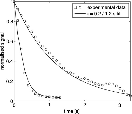
Due to limited response times of the OPCs, a correction for high frequency losses is necessary to avoid an underestimation of the eddy fluxes. The underestimated fraction is a function of both the response and the co-spectral characteristics of the scalar sensor (see Horst, 1997). Hence, to estimate the time constant of the OPCs, we conducted time response measurements, during which the OPCs’ signals were recorded during a step change in concentration. We employed a fast valve switching between two sampling intakes (one of them a zero count filter) for 20 seconds intervals. This experiment was repeated for 100 cycles. The data was then compared to the theoretical parameterisation for a first-order instrument response as derived in Doebelin (1990):2

where signal ₁ is a fixed concentration entering the instrument, signal ₂ the actual measured concentration, t is time and τ the time constant of the instrument. Transforming (2) logarithmically and applying a linear regression results in a linear equation with the slope τ⁻¹ and hence, τ can be determined. The best fit (R ²≥0.9) between the parameterisation and data was obtained for a time constant of τ=0.2 s for the UHSAS and τ=1.2 s for the PCASP-X2 (Fig. 1).

Fig. 1 Parameterised response (lines) for a first-order instrument according to Doebelin (1990) with τ=0.2 seconds and τ=1.2 seconds (lines) and averaged experimental data during a 90% step change in concentration with UHSAS (squares) and PCASP-X2 (circles).

Attenuation of the eddy fluxes was then corrected by multiplying the now solvable co-spectral transfer function with the model co-spectrum according to Horst (1997). This resulted in a median flux increase of 1% [±1.6% relative standard deviation (RSD)] for the UHSAS and 20% (±3.4% RSD) for the PCASP-X2. The commonly applied WPL correction yielded in an insignificant increase of the particle flux time series and was thus discarded.

Finally, all computed fluxes were screened and flagged by a quality assurance scheme, involving tests for instationarity (>0.3, 30% flagged; Foken and Wichura, 1996), flux kurtosis (<1 and>8, 1% flagged) and skewness (<−2 and>2, 1% flagged; Vickers and Mahrt, 1997), as well as the integral turbulence characteristics (>0.3, 10% flagged; e.g. Foken and Wichura, 1996). For all further analysis we only used quality-ensured data, which was 42% of the entire data set.

2.3. Uncertainties

Uncertainties in number concentration measurements due to discrete counting (Hinds, 1999) and the relative flux uncertainty due to limited counting statistics (Buzorius et al., 2003) were calculated as described in Deventer et al. (2013). Further, we estimated the flux uncertainty due to random instrument noise as described in Billesbach (2011) as:3 4

where primes denote deviations from the mean of the vertical wind component (w) and the target scalar (x), the number of measurements (N) within one averaging interval, and time indices i and j, where j is the index of the randomised time series. The relative uncertainty due to random noise is defined as the ratio between the measured covariance and the uncertainty covariance of w and x, where the correlation coefficient has been minimised through randomisation (in this case: 24 random permutations).

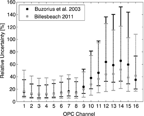
The latter one () fluctuated around 10% (median) for particles (D<160 nm), but increased gradually for bigger particles up to 50%. The relative flux uncertainty () followed the same pattern, but became slightly larger for particles (D>160 nm). In contrast, uncertainties in number concentrations were negligibly small for all particles sizes (<0.4%). To conclude, the uncertainty estimations show that flux measurements for particles with diameters D<160 nm were fairly reliable because these channels had the best counting statistics. Larger particles were far less abundant and hence, uncertainties increased and the amplitude resolution decreased. To overcome this burden to a satisfying degree, we had to classify large particles into comparably wide size classes, which limited our size resolution from the possible 140 down to 16 channels (Table 1). We decreased the amount of size classes from 19 to 16 as compared to a previous study (Deventer et al., 2013) because particle concentrations were highly variable throughout the year, whereas in the previous study we only sampled in spring.

Table 1. OPC channel classification, with geometric mean (D _m) and upper cut off diameter (D _u)

ID	D m (µm)	D u (µm)
1	0.060	0.065
2	0.069	0.074
3	0.079	0.084
4	0.088	0.093
5	0.098	0.103
6	0.108	0.112
7	0.117	0.122
8	0.131	0.141
9	0.150	0.16
10	0.170	0.179
11	0.193	0.208
12	0.222	0.236
13	0.255	0.275
14	0.294	0.313
15	0.656	1
16	1.673	10

The negligence of the assessment of storage and advection terms can yield in a further error source in surface exchange estimations (Finnigan, 2006). Formal equations of the storage term are based on the profile measurement of the scalar of interest in different heights. Instantaneous profiles are then assessed at different times (i.e. beginning and end of an EC averaging interval). During this study, particle number concentrations have only been measured on top of the tower (z=65 m). However, to estimate the storage term, we used a simple approximation as presented in Ripamonti et al. (2013). We calculated the storage term for the time window (t=14 400 seconds) between night-time minima fluxes (c ₀ at 04:00) and morning peaks (c ₁ at 08:00), because during this time the storage term was likely to be the most pronounced in contrast to the flux term, which was diminished by stable stratification and low turbulence levels:5

We calculated S for the whole dataset, median values of the relative ratio of S/F _N ranged from 5 to 39% and increased with particle diameter. This trend was the same for measurement uncertainties in both, the concentration measurement as well as the flux estimation (Fig. 2). In general, the part of the surface–atmosphere scalar flux attributed to storage was (at its maximum) within the range of relative flux uncertainties. During daytime and especially for sub-100 nm particles, S became negligible small. Due to the lack of profile measurements and the overall small contribution of S, we decided that S will not be added to F _N.

Fig. 2 Relative flux uncertainty due to limited counting statistics (black) and flux uncertainty due to random instrument noise (grey). Median values are denoted by squares with IQR error bars.

Further, the flux term due to gravitational settling (in accordance to Baron and Willeke, 2005) of the larger accumulation mode particles (D>1 µm) was estimated and was found to be significantly smaller (0.2–4.0%, inter quartile range) than the turbulent flux term (p<0.001, Kruskal–Wallis ANOVA). Thus, gravitational settling was not added to the measured fluxes.

Note that in the present study, ambient aerosol including volatile species was sampled and sized by the OPCs, meaning that the sampled air was not actively dried. Kowalksi (2001) showed that hygroscopic growth of particles due to instantaneous saturation ratio fluctuations can affect size-resolved exchange velocities in magnitudes of the measured fluxes. Vong et al. (2010) report an average change in deposition velocity due to hygroscopic growth of 0.1–0.3 cm s⁻¹ for accumulation mode particles, which corresponds to 20–60% of the median exchange velocity of accumulation mode particles measured in the present study.

3. Results and discussions

In the following text, we will use the meteorological definition of the seasons of the year. Accordingly, spring includes the months of March, April, and May, summer refers to June, July and August, the fall months are September, October and November, while the winter months are December, January and February. The weather in Münster followed the typical seasonality of temperate European climate.

3.1. Atmospheric stability, energy and CO₂ fluxes

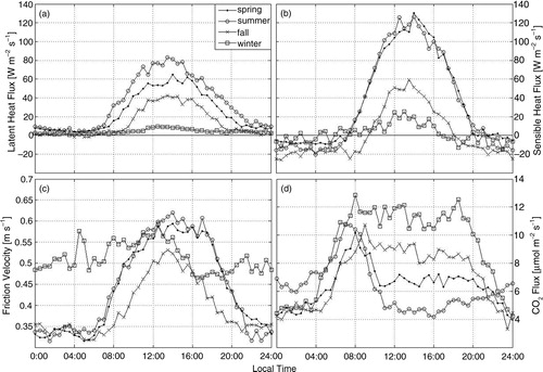
The daily course of atmospheric stability (in this study quantified by the dimensionless stability parameter ζ=(z−d)/L with measurement height (z), zero plane displacement height (d)=0.9·z _h, and Obukhov-Length (L)) varied notably throughout the year (Fig. 3). During spring and summer, a distinct pattern was apparent: from early morning (08:00) onwards, ζ became negative (weakly unstable) with an unstable midday peak (ζ<−0.55). In the afternoon, ζ increased towards neutral values until it finally reached positive (stable) values around 21:00. During the night, the urban boundary layer was constantly stable In fall, this pattern shifted towards larger values of ζ. Thus, the midday peak was only weakly unstable and during night time, ζ rose into the very stable class. Additionally, the timespan of stable conditions increased significantly. In November, unstable conditions were only established for 3 hours, as compared to 12 hours in spring and summer. From winter onwards, the nights became less stable and the time span of negative ζ increased again. Note that winter nights were the least stable. As expected, latent and SH fluxes (Fig. 4a and b) followed a yearly pattern with maxima in summer and minima in winter. Analogously to ζ, the time span of positive SH fluxes was the longest in summer (08:00–20:00) and the shortest in fall (9:00–18:00). The same pattern occurred in the seasonally-averaged friction velocity (Fig. 4c). During winter, the friction velocity oscillated around a constant value of 0.5 m s⁻¹ and no distinct diurnal course was apparent. To summarise, a yearly pattern of turbulence production was found with most pronounced and long-lasting turbulence in spring and summer. During fall, the thermal production of turbulence was diminished in magnitude and reduced time span. In winter, shear force was constantly high throughout the whole day, whereas sensible and latent heat fluxes were diminished to their yearly minima. To further characterise the urban study site, we included flux calculations of carbon dioxide (Fig. 4d). Sources for urban PM and CO₂ are often considered to be similar in cities (Järvi et al., 2009; Vogt et al., 2011a). Daily CO₂ flux patterns exhibited minima during the vegetation phase at noon (4 µmol m⁻² s⁻¹) and maxima in winter during the morning and evening rush hours and at 12:00 (≥12 µmol m⁻² s⁻¹). The yearly pattern of CO₂ fluxes had a similar course to the one of particle number concentrations.

Fig. 3 Averaged atmospheric stability classified according to Foken (2008) as ζ=(z−d)/L. Very unstable: ζ<−1.83 <, unstable: −0.55>ζ>−1.83, weak unstable: −0.55>ζ>−1.183, neutral: −0.183>ζ<−0.011, weak stable: 0.011<ζ<0.22, stable: 0.22<ζ<0.917, very stable: ζ>0.917.

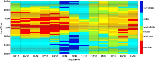
Fig. 4 Averaged daily patterns of latent heat fluxes (a), sensible heat fluxes (b), friction velocity (c) and CO₂ fluxes (d) for the different seasons: spring (dots), summer (circles), fall (crosses) and winter (squares).

3.2. Particle number concentrations N

3.2.1. Total N

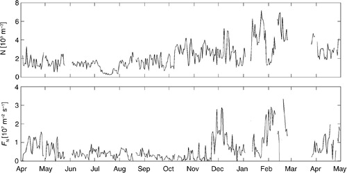
Particle number concentrations followed a typical cyclicality: maxima were recorded in January and February with monthly averages of 4.1e+09 m⁻³ and maxima daily averages of 6.5e+09 m⁻³ respectively. During spring, N declined reaching the minimum monthly (0.8e+09 m⁻³) and daily (0.5 1e+09 m⁻³) averages in July, whereas from October onwards, N increased back towards the winterly maxima (Fig. 5). This is a commonly observed pattern for European cities (e.g. Wehner and Wiedensohler, 2003; Hussein et al., 2004; Gomez-Moreno et al., 2011) and was established by (1) a more stable urban boundary layer with less turbulent mixing and less dilution throughout the cold season and (2) by an increase in urban emission activity such as domestic heating and traffic. The noticeably low concentrations in July might have been related to the above average amount of precipitation, comparably high wind speeds, and less traffic activity during to the most prominent vacation time.

Fig. 5 Daily averages of particle number concentrations (N) and fluxes (F _N) throughout the 1-yr measurement period.

3.2.2. Size-resolved N

Particle number size distributions (PNSD) commonly showed the major mode at 0.09–0.1 µm particle diameter (Fig. 6). For a comparison of two different land use sectors, the dataset was divided into a strictly urban versus a suburban class, based on the source regions of the sampled air. Suburban winds typically led to bi-modal size distributions. The minor mode was comprised of accumulation mode particles with D _m≈0.4–0.6 µm. In fall and winter, bi-modality was also apparent for urban PNSD, but generally less pronounced. The shape of the size distributions suggests that the air masses arriving at the 65 m measurement height were depleted in nucleation-mode particles. However, size-resolved measurements for particles D _m<0.06 µm were not performed and hence we can only speculate. A possible explanation for the observed shape could lie in the elevated measurement height. In urban environments, secondary particle formation usually takes place close to the precursor gas emissions and happens within short timescales (<1 second), i.e. at street level (Rönkkö et al., 2006). Previous observations on towers in urban environments support this thesis. For London (UK), Dall'Osto et al. (2011) report the smallest-particle major mode within the PNSD, as measured 160 m above street level, at 0.1 µm particle diameter. These particles were comprised of involatile graphitic compounds from engine exhaust. Synchronous street level measurements, on the other hand, resulted in a major peak within the nucleation mode (D<30 nm). For the Münster data presented here, an influence of traffic is still apparent since urban PNSD generally peaked at smaller particle diameters than suburban ones. The trend of a more pronounced bi-modality of the suburban size distributions suggests that the larger accumulation mode particles originated from regional background and long range transport. Time series analysis (Deventer et al., 2013) supports this thesis. As presented in Section 2.1, suburban winds coincided with stable stratifications and long-lasting stable weather conditions. Hence, the comparably high suburban N were established by accumulation of aged background particles and long range transport in the stable boundary layer, which favoured positive contribution of far-distant sources and hence larger concentration footprint sizes. This explains why suburban particle number concentrations, in contrast to the respective number fluxes, were on average higher than urban number concentrations (Fig. 6; Table 2.), which were more directly controlled by daily emission and turbulence patterns. The observation also shows that urban fluxes can have a different flux source sector than the respective number concentrations (see Ripamonti et al., 2013).

Fig. 6 Averaged particle number size distributions (PNSD) expressed as ensemble log normal distributions for the different seasons: spring (light grey, thick line), summer (medium grey), fall (dark grey), and winter (black). Urban size distributions (solid lines) vs. suburban ones (dashed lines).

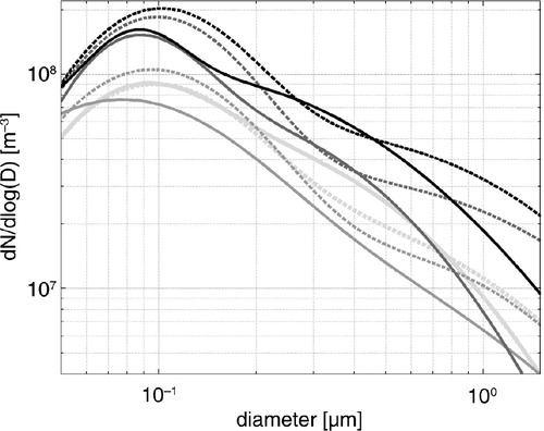
Table 2. Median and IQR (in brackets) of total particle number fluxes (F _N), concentrations (N) and stability parameter (ζ) for the different seasons and for two different land use sectors. Inter-source region significance with *(p<0.05, Kruskal–Wallis ANOVA) and inter-season significance (ABCD).

	Spring	Summer	Fall	Winter	Sig.
Urban
F N [e+06 m^−2 s^−1]	7.50* (3.1, 13.16)	5.17* (2.08, 9.24)	2.91* (−0.53, 8.25)	10.4* (4.2, 19.9)	ABCD
N [e+09 m^−3]	1.36 (1.03, 2.05)	1.05* (0.53, 1.47)	1.84* (1.18, 2.65)	2.1* (1.4, 3.3)	ABCD
ζ=(z–d)/L	−0.1052* (−0.327, 0.032)	−0.0879* (−0.286, 0.044)	0.007* (−0.137, 0.260)	−0.004* (−0.086, 0.056)	AABC
Suburban
F N [e+06 m^−2 s^−1]	3.1* (0.98, 7.1)	1.72* (0.41, 4.75)	0.39* (−1.22, 3.12)	4.6* (1.3, 10.4)	ABCD
N [e+09 m^−3]	1.30 (1.02, 1.76)	1.45* (1.03, 1.79)	2.64* (1.77, 3.27)	3.33* (2.51, 4.63)	AABC
ζ=(z−d)/L	−0.0387* (−0.289, 0.223)	−0.0084* (−0.537, 0.629)	0.429* (0.039, 1.391)	0.157* (−0.002, 0.624)	AABC

3.2.3. N – Daily patterns

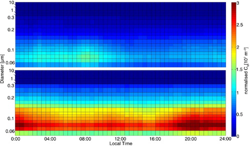
Size-resolved particle number concentrations exhibited daily patterns which varied in the different seasons (Fig. 7). In spring and summer, N continuously rose over the night from 18:00 until the morning peak at 8:00. Particles with diameters between 0.06 and 0.09 µm reached maxima concentrations. From then on the concentrations sharply decreased and fluctuated around a minimum plateau from 13:30 to 17:30, before they finally started to increase again. This pattern applied to particles of the entire size spectrum. In winter, the size-resolved N course had different characteristics. Firstly, N started to rise comparably early from 16:30 onwards. Secondly – in contrast to spring and summer – the increase in N was not continuous. For particles smaller than 0.12 µm, it stopped at 21:00. From then on, the concentrations decreased. N of larger particles, on the other hand, kept increasing until they reached a maximum at 22:00. This divergent course can be explained by coagulation and growth processes in the stable boundary layer, which led to a decrease of traffic-related ultrafine particles and a synchronous increase in accumulation mode particle numbers during night-time. Thirdly, a local maximum was reached at 10:30. From then on, N decreased until they finally started rising again at 16:30.

Fig. 7 Averaged diurnal courses of normalised size-resolved number concentrations (N) for summer (top panel) and winter (lower panel). Y-Axes in log scale and non-continuous.

3.3. Particle number fluxes (F _N)

3.3.1. Total F _N

Total particle number fluxes followed a seasonal pattern similar to the one of total N. Maximum fluxes occurred in winter with daily averages of up to 3.0e+07 m⁻² s⁻¹ (Fig. 5). In contrast to N, the fluxes steadily decreased from spring onwards until they abruptly increased late November. Hence, the smallest fluxes (~2.0e+06 m⁻² s⁻¹) were observed during October. It is apparent that during fall, the boundary layer was mostly stable and turbulent mixing was limited to only a few hours per day (Fig. 3). Simultaneously, the friction velocities reached minimum values (Fig. 4c). As a result, particles could continuously accumulate below and above the measurement site, which consequently led to a diminished gradient between particle source and sink regions, which ultimately led, together with the diminished turbulence production, to the observed minima in F _N. To the recent date, results from long-term particle fluxes are rare, hence a comparison of our data is limited to reports of Järvi et al. (2009), Vogt et al. (2011b) and Ripamonti et al. (2013), who observed a likewise annual flux pattern (with maxima in winter). However, Vogt et al. (2011b) could only find a clear seasonality for super-micrometre particles peaking in winter, which they partly attribute to wood burning emissions. The winter maxima of F _N were established by multiple factors. Firstly, the urban particle sources were most active during this season. Besides elevated emissions from traffic due to the cold temperatures (i.e. discussed in Virtanen et al., 2006), the city was exposed to enhanced emissions from the energy production sector as well as from wood burning for domestic heating (BRMS.NRW, 2009). Secondly, Dall'Osto et al. (2011) observed shifts in size distributions from street level to tower measurements, which were explained by evaporation processes of semi-volatile nano-particles from traffic emissions. Accordingly, lower temperatures enhance traffic emissions and ultrafine particle concentrations due to a weakened evaporational loss. Overall, F _N exhibits a course similar to that of N, with the exception of divergent development in fall.

Total particle fluxes (usually in the operation range of a commercial condensation nuclei counter (CPC), which is usually between 0.007 µm and a few micrometres in diameter) have been assessed in various medium-sized to major European cities (Nemitz et al., 2000, Dorsey et al., 2002; Longley et al., 2004; Mårtensson et al., 2006; Järvi et al., 2009; Martin et al., 2009; Dahlkötter et al., 2010; Ripamonti et al., 2013) and were found to be almost exclusively positive. Consequently cities were characterised as relevant particle sources. A comparison of absolute values of F _N between the previous studies and ours is not feasible because different instruments covering different particle size ranges were used. Harrison et al. (2012) report that fluxes derived from UHSAS measurements covered 10% up to about 100% of total fluxes as measured with a CPC and that the flux ratio (F _UHSAS/F _CPC) showed clear temporal variability. On the other hand, it can be stated that among previously published papers and the present study at least the magnitude of number fluxes is consistent and that the measured particle number concentrations are in good agreement. During the Münster campaign, negative total number fluxes (particle deposition) were recorded during 13% of the time series and were notably smaller in magnitude (median: −1.1e+06 m⁻² s⁻¹) than the positive ones (median: 5.8e+06 m⁻² s⁻¹). On several days (mostly in summer), bulk particle number fluxes were governed by particle deposition. Particle deposition proved to be frequently occurring and contributed at least temporarily considerably to the total flux and was thus not neglected in the overall data analysis.

3.3.2. Size-resolved F _N

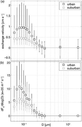
The particle fluxes varied notably with particle size. Figure 8 shows that both the exchange velocities (ve) as well as the particle fluxes (F _N) peaked for ultrafine particles (D _m=0.88 µm; median ve=1.0 (0.4–2.1) cm s⁻¹) and decreased both with increasing and decreasing particle size. Minimum exchange velocities were observed for smaller accumulation mode particles (D _m=0.15 µm). While the majority of ve of the smaller particles were strictly positive, bi-directional fluxes were observed for particles with diameters D _m≥0.17 µm. From here on, the diameter above which negative fluxes occurred, is called ‘tipping-point’. With diameters increasing above the tipping point, positive and negative exchange velocities increased. A comparison of the observed flux size distributions to other studies is difficult, since size-resolved urban particle flux observations are still sparse and negative fluxes are generally not addressed (Noone et al., 2003; Schmidt and Klemm, 2008; Vogt et al., 2011a, 2011b; Harrison et al., 2012; Deventer et al., 2013). For Stockholm Vogt et al. (2011a) report a similar pattern, with a peak in number fluxes for the smallest particle size class analysed (0.25 µm) and a decrease throughout the accumulation mode. For super micrometre particles, a weak increase in flux magnitudes was observed. Harrison et al. (2012), also employing a UHSAS, report a pattern with maxima emission velocities for ultrafine particles as well as for particles at the upper end of the UHSAS size spectrum, which is in general agreement to our results. Schmidt and Klemm (2008) observed frequent deposition of accumulation mode particles, which led to a net particle mass deposition on days with net particle number emission. This seemingly contradictory observation was confirmed in Deventer et al. (2013) and in the present study.

Fig. 8 Size-resolved particle exchange velocities (a) and fluxes (b) with median (symbols) and 25th/75th percentiles (error bars) differentiated in two source regions: urban (black) and suburban (grey).

3.3.3. F _N and F _M – Daily patterns

Particle number fluxes (F _N) as well as particle mass fluxes (F _M) showed a well-established daily cyclicality. Averaged daily patterns are plotted in Figs. 9 and 10 for each season separately. A common feature of all F _N courses is a steep increase in the early morning hours, followed by fluctuations around a plateau from 08:00 onwards, a decrease between 20:00 and 24:00, and near-zero values for the rest of the night. The negligible fluxes during night were attributable to receding turbulence production and the resulting stable nocturnal boundary layer (Figs. 4 and 5). A previous study in Münster identified, that the peak in F _N occurred synchronously with the morning rush hour (Dahlkötter et al., 2010). Our data further show that the morning (06–08 hours) increase in F _N was facilitated by convective venting of the shallow and mostly stable nocturnal boundary layer. During this time, total F _N were predominantly driven by UFP smaller than 0.12 µm (Fig. 10). A close relation between traffic activity and peaks in particle number fluxes during the morning hours is a typical observation and hence traffic activity was implemented in empirical flux parameterisations (Dorsey et al., 2002; Mårtensson et al., 2006; Järvi et al., 2009; Martin et al., 2009).

Fig. 9 Averaged daily patterns of total number (green) and total mass flux (blue) during the four seasons. Filled areas (inter quartile range) symbolise the day-to-day variation. Single 30-minute averages and respective variances are calculated from 33 (min) to 51 (max) data points, according to results from the quality control scheme (Section 2.1).

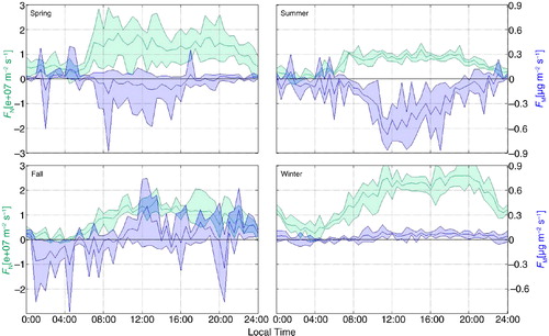
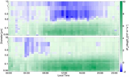
Fig. 10 Averaged diurnal courses of size-resolved number fluxes (F _N) for summer (top panel) and winter (lower panel). Y-Axes in log scale and non-continuous.

Daily patterns of particle fluxes varied notably throughout the year. The characteristic morning increase at 8 hours was steepest during spring. A discrete characteristic of the winter pattern was an almost continuous increase in F _N, reaching the maxima comparably late (between 12 and 18 hours), in contrast to the more stable plateau pattern in spring and summer. The reason for this was the less pronounced diurnal pattern of turbulence production in winter. In spring and summer, shear and convection increased rapidly between 06 and 8 hours. Consequently the boundary layer stratification switched from stable to (very) unstable (Fig. 5). This led to a quick emission of particles which accumulated during the night-time and particles from the morning traffic rush hour. Typically, particle fluxes do not reflect the double peak pattern which is commonly observed for traffic activity (Dorsey et al., 2002; Mårtensson et al., 2006; Järvi et al., 2009). The reason for this lies in the stronger turbulent mixing throughout the afternoon period. During this time F _N rather follow the course of SH fluxes (Martin et al., 2009). In winter, when convection was comparably low and shear force was constantly high, the transition from stable to neutral-unstable stratification was less pronounced and extended over the (after) noon period. As a result, winter F _N peak comparably late and exhibit a less steep increase during the morning hours.

Mass fluxes can be classified into a spring–summer and a fall–winter pattern, respectively (Fig. 9). The first one was opposed to the common F _N pattern, but was delayed by 3–4 hours. We observed an increase of the magnitudes of the negative mass fluxes from 08:00 onwards, followed by the largest negative fluxes around 12:00. In contrast to F _N, the magnitudes of the mass fluxes decreased shortly after reaching their minima until they fluctuated around zero from midnight onwards. Through the size-resolved fluxes (Fig. 10) it becomes apparent, that particle mass deposition was mostly driven by particles of 0.21<D _m >0.31 µm diameter. Fluxes of the indicated size range peaked at 12:30. Fall and winter patterns of F _M followed the respective F _N courses, with the exception of negative values between 02:00 and 06:00. Since F _M were driven by larger accumulation mode particles, they were not as directly linked to urban emissions as F _N and rather scaled with the diurnal pattern of turbulence production.

3.3.4. The effect of different source regions on F _N

When the flux time series was divided into a strictly urban versus a suburban class, the urban class yielded significantly higher total number fluxes (approx. by a factor of 2–3) throughout the whole year. These factors reached notably large values during fall (Table 2). The size-resolved flux measurements present an explanation for the observed differences in flux magnitudes. Whereas the shape of the pattern of F _N as a function of particle size did not differ noticeably between suburban and urban fluxes (Fig. 8), the magnitude of suburban fluxes of ultrafine particles were significantly lower. The fluxes F _N of the larger accumulation mode particles, however, were almost identical for the urban and suburban sectors. It appears that the difference of the flux magnitudes was not caused by differences in particle number concentrations: The size-resolved particle exchange velocities exhibit the same pattern as the respective particle fluxes (Fig. 8a). This leads to the hypothesis that the difference in particle emission fluxes was attributable to either different meso-scale meteorological conditions when the wind came from the urban or the suburban sector (e.g. different stability), or to different micro-meteorological conditions (e.g. more turbulence production in the urban canopy), or, most likely, to a combination of the two. According to this reasoning, accumulation mode (here: D _m>0.2 µm) fluxes were not governed by diurnal patterns of urban particle emissions and turbulence production, but were more likely driven by long-range transport and down-mixing from residual layers.

3.3.5. Deposition fluxes

In general, we observed an increase in deposition flux frequency and deposition velocities with particle size. Persistent deposition of particles with diameters larger than the tipping point (D _m>0.17 µm) was predominantly observed when the urban boundary layer reached a (very) unstable state, namely during spring and summer. During these periods, the frequently observed deposition of accumulation mode particles (relative frequency of 40–80%), which was the most pronounced between 09 and 18 hours (Fig. 10), diminished total F _N only to some degree (10–50%), but resulted in an inversion of the mass flux direction. In other words, during spring and summer, the largest part of the mass transported by particles of the assessed size spectrum was depositing, while we simultaneously observed a net emission of particle numbers. This finding gives scope for the debate about the origin and source mechanism of the depositing particles. Time series analysis of the size-resolved flux time series (not presented here) revealed that in contrast to ultrafine particles, the accumulation mode time series featured several meso-scale cycles of which the yearly cycle was the most pronounced. For ultrafine-particle flux time series, on the other hand, the daily cycle yielded the highest significance in the analysis, accordingly to Lomb-Scargle periodograms (i.e. Lomb, 1972; Schulz and Statteger, 1998; Trauth, 2006). This leads us to the conclusion that the predominantly depositing particles were to a certain degree associated with (1) meso-scale advection and (2) down-mixing from residual layers. This seems plausible, considering that during street canyon measurements of PM10 in Münster during 2006 and 2008 the contribution of PM from long range transport made up 68% of the contributions from traffic (Gietl and Klemm, 2009). During winter, when the urban boundary layer was mostly neutral to weakly unstable stratified and the mixing layer height is typically reduced (e.g. Schäfer et al., 2006), urban accumulation mode particle concentrations were enhanced due to reduced pollutant dispersion. Hence the gradient for accumulation mode particles was upward directed, which prevented pronounced deposition as observed in spring and summer.

3.4. Flux drivers and flux correlations

Among the total set of measured fluxes and meteorological parameters, the friction velocity (u*), the state of atmospheric stability (ζ), the CO₂ flux (F _CO2 ), as well as the horizontal wind speed (U) showed distinct correlations with particle exchange velocities (ve) and particle number fluxes. In general, ve reached maximum magnitudes during periods with high wind speeds and a neutral stability (in this study: −0.183<ζ<0.01). In theory, these conditions lead to maxima of u*, which increases with U and peaks at neutral stratification. Corresponding to this formal relation, an acceptable linear increase of ve with increasing u* was found in the particle flux time series. The linear relation was apparent for positive as well as negative particle fluxes of all presented size classes (Fig. 11a), but was generally stronger for emission fluxes. The correlation itself was not sensitive to the source region differentiation. Strongest relations (maximum slopes of the linear fit) were found for ultrafine particles and for the largest size fraction analysed in this study. This is in good agreement to previous studies. Martin et al. (2009) and Vogt et al. (2011b) report a linear relation, whereas Mårtensson et al. (2006) report a non-linear power-function.

Fig. 11 Median correlation of exchange velocity and bin-aggregated flux drivers friction velocity u* (a), wind speed U (b), stability parameter ζ (c) and CO₂ flux (d) with the respective coefficients for a linear regression: y=p1 x+p2, and a second-order polynom: y=p1 x2+p2 x+p3. Grey scale denotes particle diameter from light grey (0.06 µm) to black (1 µm). Ultrafine particles (triangles), accumulation mode particles (circles), and super micrometre particles (squares).

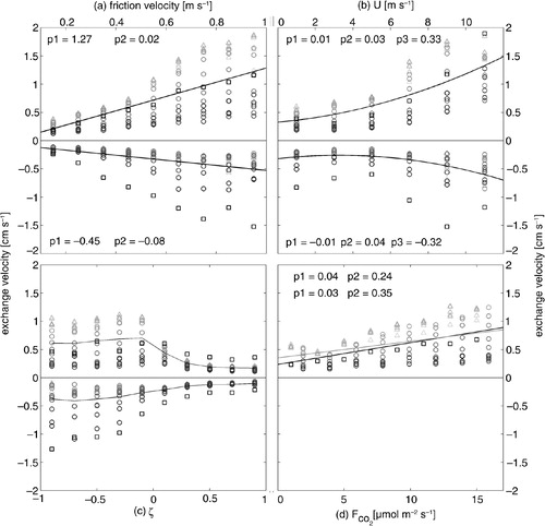
Analogously, emission velocities increased with increasing wind speeds. In this case, a second-order polynomial resulted in a better fit (Fig. 10b). Interestingly, the strongest relation was found for the largest size class, which might be related to re-suspension of super micrometre particles like road dust (i.e. Järvi et al., 2009b; Vogt et al., 2011a). The increase in negative ve for the lowest bin of U might be related to comparably poor data coverage for periods with near-zero wind speeds.

The relation of ve and the dimensionless stability parameter ζ was more complex (Fig. 10c). For positive values of ζ, the exchange velocities were near to zero. For values of ζ corresponding to a weakly stable to neutral stratification, positive ve increased sharply. With a further decreasing ζ (unstable to very unstable stratification, ζ<−0.2), ve fluctuated around a plateau. Negative fluxes showed a similar but less pronounced pattern and reached the plateau for higher negatives values of ζ. For the size classes D _m≥0.275 µm, the data suggests a linear increase in deposition fluxes with decreasing stability. Again the observed relations did not change notably, when the dataset was divided into suburban and urban fluxes. The observed minima of total F _N during fall are a good showcase for the link between local meteorology and atmospheric conditions on particle emissions: The mostly stable atmosphere with low friction velocities diminished F _N, even though urban sources were likely more active than in summer, as reflected by enhanced particle number concentrations for all size classes.

Latest studies on urban particle fluxes reported positive linear correlations of CO₂ fluxes and particle emissions (e.g. Järvi et al., 2009; Vogt et al., 2011b; Contini et al., 2012). This is especially the case for studies, in which condensation particle counters (CPC) were used to measure nucleation mode particles close to street canyons. Järvi et al. (2009) report a R ² of up to 0.34/0.6 for an urban/road sector in Helsinki at 40 m measurement height and a lower detection limit of the CPC of about 6 nm. The same applies to the study from Contini et al. (2012), who employed a CPC EC set-up 14 m above street level and reported a Pearson correlation coefficient of r=0.56. If all data from the present study are taken into account, the correlation of ve and F _CO2 was comparably weak, with a maximum r of 0.41 and R ² of 0.17 in the winter time. The differentiation in urban and suburban fluxes had a significant effect on the estimated relations with ve, which decreased to r=0.13/R ²=0.02 for the suburban sector. Further, the correlation coefficients showed a seasonal/yearly pattern and were the weakest during the growing period. This pattern becomes conclusive before the background of the diurnal and seasonal patterns of the CO₂ fluxes. In Münster, the CO₂ uptake of the vegetation can be in the same order of magnitude as CO₂ emissions from traffic and as a result, spring and summer time CO₂ fluxes were low or negative (single 30-minute values) during noon and the afternoon (Fig. 4d) even for the urban flux sector. At the same time, particle fluxes peaked, resulting in a poor correlation. However, the correlation coefficients could be improved, when the flux time series was filtered for positive CO₂ and positive particle fluxes. The results suggest a linear increase in ve with increasing CO₂ emissions (Fig. 11d, black fit). Since the CO₂ fluxes inter-correlated with the turbulence parameters, we normalised F _CO2 with u*. The results suggest that a relation to ve (grey fit) was less pronounced but still justifiable without the influence of turbulence drivers, which supports the thesis that urban particle and CO₂ emissions have, to some degree, the same source mechanisms (most prominently traffic, e.g. Dorsey et al., 2002; Mårtensson et al., 2006; Dahlkötter et al., 2010; Järvi et al., 2009; Martin et al., 2009; Vogt et al., 2011a). This thesis is further supported by the fact that ultrafine particles, which likely originated from traffic emissions, showed the strongest correlations with CO₂ fluxes (grey triangles, Fig. 11d).

4. Summary and conclusions

For a period of 1 yr, particle number concentrations for particles with diameters between 0.06 and 10 µm were measured over an urban area. The particle number and mass fluxes for 16 different size classes were calculated directly using the EC method. Overall, the studied city was a particle source with maxima aggregated emission fluxes of 10.4e+06 m⁻² s⁻¹ in winter and minima of 2.91e+06 m⁻² s⁻¹ during fall. Particle emissions followed a distinct diurnal pattern, which was closely related to turbulence production. Size-segregated flux measurements revealed that accumulation mode particles with diameters>0.17 µm frequently deposited during spring and summer. This could lead to bi-directional fluxes of particle number (emission) and particle mass (deposition). Within a comprehensive analysis including energy fluxes, stability approximations, meteorological parameters, time series algorithms, and footprint classification, we searched for driving factors, correlations, and temporal patterns of fluxes and concentrations. Our results show that urban particle number fluxes were strongly linked to the friction velocity and horizontal wind speed, atmospheric stability, and source activity. Since these driving factors varied considerably throughout the year, the analysed particle flux time series followed a clear seasonality. Strongest and quasi linear relations were found with the friction velocity. However, not all of the identified flux drivers had a linear effect on particle fluxes. Divergent trends in particle number fluxes and concentrations were apparent in fall, when turbulent mixing was substantially reduced. The resulting accumulation of particles did not lead to an increase in particle fluxes. This leads us to the conclusion that for a comprehensive perspective on urban particle fluxes, we need to analyse them within a multi-dimensional framework. Because the mass/number ratio is much larger for bigger particles than for small particles, the particle mass fluxes scale within any of the identified flux drivers in a different way than particle number fluxes. It is not feasible to study particle fluxes along either one of the mentioned driving factors alone, because their impact on particles fluxes is strongly inter-correlated. Our results specifically emphasise the importance of size-resolved flux measurements because the various drivers of particle fluxes acted differently on particles of different sizes. Multiple mechanisms (e.g. bi-directional fluxes) can be camouflaged within a total flux measurement covering a wide particle size spectrum containing particles of a variety of sources and age.

Acknowledgements

This study was supported by the German Science Foundation (DFG) through contract KL623/12. We further thank Roland Balthasar on behalf of the Bundeswehr for the possibility to use their radio tower. Furthermore, we would like to thank S. Heupel Santos, C. Stader and ILÖK staff for support during field work. Thanks to two anonymous reviewers who gave helpful comments on an earlier version of the manuscript.

References

- Baron P. A. , Willeke K . Aerosol Measurement: Principles, Techniques, and Applications.
- BRMS.NRW. Air quality directive for the city of Münster. [District Government]. 2009. Online at: http://www.bezreg-muenster.nrw.de/startseite/abteilungen/abteilung5/Dez_53_Immissionsschutz_einschl_anlagenbezogener_Umweltschutz/Luftqualitaetsplan_Muenster/ .
- Buzorius G. , Rannik Ü. , Mäkelä M. , Vesala T. , Kulmala M . Vertical aerosol particle fluxes measured by eddy covariance technique using condensational particle counter. J. Aerosol Sci. 1998; 29: 157–171.
- Buzorius G. , Rannik Ü. , Nilsson E. D. , Vesala T. , Kulmala M . Analysis of measurement techniques to determine dry deposition velocities of aerosol particles with diameters less than 100 nm. J. Aerosol Sci. 2003; 34: 747–764.
- Contini D. , Donateo A. , Elefante C. , Grasso F. M . Analysis of particles and carbon dioxide concentrations and fluxes in an urban area: correlation with traffic rate and local micrometeorology. Atmos. Environ. 2012; 46: 25–35.
- Dahlkötter F. , Griessbaum F. , Schmidt A. , Klemm O . Direct measurement of CO(2) and particle emissions from an urban area. Meteorol. Z. 2010; 19(6): 565–575.
- Dall'Osto M. , Thorpe A. , Beddows D. C. S. , Harrison R. M. , Barlow J. F. , co-authors . Remarkable dynamics of nanoparticles in the urban atmosphere. Atmos. Chem. Phys. 2011; 11: 6623–6637.
- Deventer M. J. , Griessbaum F. , Klemm O . Size-resolved flux measurement of sub-micrometer particles over an urban area. Meteorol. Z. 2013; 6(22): 729–737.
- Doebelin E. O . Measurement Systems. 1990; New York: McGraw-Hill. 104–194.
- Dorsey J. R. , Nemitz E. , Gallagher M. W. , Fowler D. , Williams P. I. , co-authors . Direct measurements and parameterisation of aerosol flux, concentration and emission velocity above a city. Atmos. Environ. 2002; 36: 791–800.
- Finnigan J . The storage term in eddy flux calculations. Agr. Forest Meteorol. 2006; 136: 108–113.
- Foken T . Micrometeorology. 2008; Berlin: Springer. 235.
- Foken T. , Wichura B . Tools for quality assessment of surface-based flux measurements. Agr. Forest Meteorol. 1996; 78(1–2): 83–105.
- Gallagher M. , Beswick K. M. , Duyzer J. , Westrate H. , Choularton T. , co-authors . Measurements of aerosol fluxes to Speulder forest using a micrometeorological technique. Atmos. Environ. 1997; 31: 359–373.
- Gallagher M. , Fontan J. , Wyers P. , Ruijgrok W. , Duyzer J. , co-authors . Slanina S . Atmospheric particles and their interactions with natural surfaces. Biosphere-Atmosphere Exchange of Pollutants and Trace Substances. 1997b; Berlin: Springer-Verlag. 45–92.
- Gietl J. K. , Klemm O . Source identification of size-segregated aerosol in Münster, Germany, by factor analysis. Aerosol Sci. Tech. 2009; 43: 828–837.
- Gietl J. K. , Tritscher T. , Klemm O . Size-segregated analysis of PM10 at two sites, urban and rural, in Münster (Germany) using five-stage Berner type impactors. Atmos. Environ. 2008; 42: 5721–5727.
- Gomez-Moreno F. J. , Pujadas M. , Plaza J. , Rodríguez-Maroto J. J. , Martínez-Lozano P. , co-authors . Influence of seasonal factors on the atmospheric particle number concentration and size distribution in Madrid. Atmos. Environ. 2011; 45: 3167–3180.
- Griessbaum F. , Schmidt A . Advanced tilt correction from flow distortion effects on turbulent CO2 fluxes in complex environments using large eddy simulation. Q. J. Roy. Meteorol. Soc. 2009; 135: 1603–1613.
- Harrison R. M. , Dall'osto M. , Beddows D. C. S. , Thrope A. J. , Bloss W. J. , co-authors . Atmospheric chemistry and physics in the atmosphere of a developed megacity (London): an overview of the REPARTEE experiment and its conclusions. Atmos. Chem. Phys. 2012; 12: 3065–3114.
- Held A. , Hinz K. , Trimborn A. , Spengler B. , Klemm O . Towards direct measurement of turbulent vertical fluxes of compounds in atmospheric aerosol particles. Geophys. Res. Lett. 2003; 30(19): 8/1–8/4.
- Hicks B. B. , Wesley M. L. , Durham J. L. , Brown M. A . Some direct measurements of atmospheric sulfur fluxes over a pine plantation. Atmos. Environ. 1982; 16: 2899–2903.
- Hinds W. C . Aerosol Technology. Properties, Behavior, and Measurement of Airborne Particles. 2nd ed . 1999; New York: Wiley. 483.
- Horst T. W . A simple formula for attenuation of eddy fluxes measured with first-order-response scalar sensors. Boundary Layer Meteorol. 1997; 82: 219–233.
- Hussein T. , Puustinen A. , Aalto P. P. , Mäkelä J. M. , Hämeri K. , co-authors . Urban aerosol number size distributions. Atmos. Chem. Phys. 2004; 4: 391–411.
- Järvi L. , Hannuniemi H. , Hussein T. , Junninen H. , Aalto P. P. , co-authors . The urban measurement station SMEAR III: continuous monitoring of air pollution and surface-atmosphere interactions in Helsinki, Finland. Boreal Environ. Res. 2009b; 14: 86–109.
- Järvi L. , Rannik Ü. , Mammarella I. , Sogachev A. , Aalto P. P. , co-authors . Annual particle flux observations over a heterogeneous urban area. Atmos. Chem. Phys. 2009; 9(20): 7847–7856.
- Katen P. C. , Hubbe J. M . An evaluation of optical particle counter measurements of the dry deposition of atmospheric aerosol particles. J. Geophys. Res. 1985; 90: 2145–2160.
- Kowalksi A. S . Deliquescence induces eddy covariance and estimable dry deposition errors. Atmos. Environ. 2001; 35: 4843–4851.
- Lomb N. R . Least-squared frequency analysis of unequally spaced data. Astrophys. Space Sci. 1972; 39: 447–462.
- Longley I. D. , Gallagher M. W. , Dorsey J. D. , Flynn M . A case-study of fine particle concentrations and fluxes measured in a busy street canyon in Manchester, UK. Atmos. Environ. 2004; 38: 3595–3603.
- Mårtensson E. M. , Nilsson E. D. , Buzorius G. , Johansson C . Eddy covariance measurements and parameterization of traffic related particle emissions in an urban environment. Atmos. Chem. Phys. 2006; 6: 769–785.
- Martin C. L. , Longley I. D. , Dorsey J. R. , Thomas R. M. , Gallagher M. W. , co-authors . Ultrafine particle fluxes above four major European cities. Atmos. Environ. 2009; 43: 4714–4721.
- Nemitz E. , Jimenez J. L. , Huffman A. , Ulbrich I. M. , Canagaratna M. R. , co-authors . An eddy-covariance system for the measurement of surface/atmosphere exchange fluxes of submicron aerosol chemical species – first application above an urban area. Aerosol Sci. Tech. 2008; 42: 636–657.
- Nemitz E. , Williams P. I. , Theobald M. R. , McDonald A. G. , Fowler D. , co-authors . Midgley P. M. , Reuther M. , Williams M . Application of two micrometeorological techniques to derive fluxes of aerosol components above a city. EUROTRAC–2 Symposium 2000.
- Noone K. J. , Baltensperger U. , Flossmann A. I. , Fuzzi S. , Hass H. , co-authors . Midgley P. M. , Builtjes P. J. H. , Harrison R. M. , Tørseth K . Tropospheric aerosols and clouds. Towards Cleaner Air for Europe – Science, Tools and Applications. 2013; Weikersheim: Margraf Publishers. 157–194.
- Pitz M. , Cyrys J. , Karg E. , Wiedensohler A. , Wichmann H. E. , co-authors . Variability of apparent particle density of an urban aerosol. Environ. Sci. Tech. 2003; 37: 4336–4342.
- Pryor S. C. , Gallagher M. , Sievering H. , Larsen S. E. , Barthelmie R. J. , co-authors . A review of measurement and modelling results of particle atmosphere–surface exchange. Tellus B. 2008; 60: 42–75.
- Ripamonti G. , Järvi L. , MØlgaard B. , Hussein T. , Nordbo A. , co-authors . The effect of local sources on aerosol particle number size distribution, concentrations and fluxes in Helsinki, Finland. Tellus B.
- Schäfer K. , Emeis S. , Hoffmann H. , Jahn C . Influence of mixing layer height upon air pollution in urban and sub-urban areas. Meteorol. Z. 2006; 15: 647–658.
- Schmidt A. , Klemm O . Direct determination of highly size-resolved turbulent particle fluxes with the disjunct eddy covariance method and a 12-stage electrical low pressure impactor. Atmos. Chem. Phys. 2008; 8: 7405–7417.
- Schulz M. , Stattegger K . SPECTRUM. Spectral analysis of unevenly spaced paleoclimatic time series. Comput. Geosci. 1998; 23: 929–945.
- Trauth M. H . MATLAB Recipes for Earth Sciences. 2nd ed . 2006; Berlin: Springer Verlag. 83–132.
- Vickers D. , Mahrt L . Quality control and flux sampling problems for tower and aircraft data. J. Atmos. Ocean. Technol. 1997; 14(3): 512–526.
- Virtanen A. , Rönkkö T. , Kannosto J. , Ristimäki J. , Mäkelä J. M. , co-authors . Winter and summer time size distributions and densities of traffic-related aerosol particles at a busy highway in Helsinki. Atmos. Chem. Phys. 2006; 6: 2411–2421.
- Vogt M. , Nilsson E. D. , Ahlm L. , Martensson E. M. , Johansson C . The relationship between 0.25–2.5 mu m aerosol and CO(2) emissions over a city. Atmospheric Chem. Phys. 2011a; 11: 4851–4859.
- Vogt M. , Nilsson E. D. , Ahlm L. , Mårtensson E. M. , Johansson C . Seasonal and diurnal cycles of 0.25–2.5 µm aerosol fluxes over urban Stockholm, Sweden. Tellus B. 2011b; 63: 935–951.
- Vong R. J. , Vong I. J. , Vickers D. , Covert D. S . Size-dependent aerosol deposition velocities during BEARPEX'07. Atmos. Chem. Phys. 2010; 10: 5749–5758.
- Wehner B. , Wiedensohler A . Long term measurements of submicrometer urban aerosols: statistical analysis for correlations with meteorological conditions and trace gases. Atmos. Chem. Phys. 2003; 3: 867–879.