ENSO-related variability in latitudinal distribution of annual mean atmospheric potential oxygen (APO) in the equatorial Western Pacific

Abstract

We examined temporal variations in the latitudinal distribution of annual mean atmospheric potential oxygen (APO=O₂+1.1×CO₂), a useful tracer for studying ocean biogeochemical processes. To compute APO, we used atmospheric CO₂ and O₂ concentrations from flask samples and in-situ measurements onboard commercial cargo ships sailing between Japan and Australia/New Zealand. Most of the observed latitudinal distributions of the annual mean APO for the years 2002–2012 showed equatorial bulges, indicating tropical APO outgassing fluxes. However, the equatorial bulge was noticeably absent during the 2009/2010 El Niño period, especially in the Southern Hemisphere. The temporal variation in the 25–0°S latitudinal APO gradient correlated significantly with the El Niño/Southern Oscillation (ENSO); the equatorward APO gradients decreased (increased) during the El Niño (La Niña) period with a variability of about ±0.1 per meg/degree. Simulated APO based on an atmospheric transport model driven by climatological/constant flux fields and reanalysis meteorological data reproduced the overall characteristic of the observed temporal variation in the APO gradients well, suggesting that the atmospheric transport contributed substantially to the observed interannual variation in the global APO distributions. However, the model simulation underestimated the variability in the APO gradients by about 25%, compared to the observations. These discrepancies suggest a possibility of the existence of additional APO flux variability in the tropical Pacific, enhancing the ENSO-related variability in the observed APO gradients.

• air–sea gas exchange
• atmospheric O₂/N₂ ratio
• APO
• ENSO
• atmospheric transport
• shipboard observation

1. Introduction

Measurements of the atmospheric O₂ concentration, combined with the atmospheric CO₂ concentration, have been shown to be significantly useful in constraining global carbon budgets (e.g. Keeling and Shertz, 1992; Battle et al., 2000; Bender et al., 2005; Manning and Keeling, 2006). This is based on the fact that there exists a tight coupling between O₂ and CO₂ fluxes during land biotic processes (photosynthesis and respiration) while oceanic O₂ and CO₂ fluxes are decoupled, because the buffering effect of the carbonate chemistry in the ocean suppresses the air−sea exchange of CO₂ (cf. Keeling et al., 1993). The tight coupling in the land biotic processes can be approximately reproduced by using the associated CO₂ change and the biotic −O₂:CO₂ exchange ratio (Keeling et al., 1998b). Based on this idea, Stephens et al. (1998) defined a tracer of atmospheric potential oxygen (APO) as APO=O₂+1.1×CO₂, where 1.1 represents the molar land biotic −O₂:C exchange ratio (Severinghaus, 1995), thus eliminating the influence of the biosphere. Since APO is invariant with respect to the land biotic exchange, its variations therefore mainly reflect the variations in the air-to-sea gas exchange. Note that fossil fuel burning causes slight spatio-temporal variations in APO for the global long-term decrease and the inter-hemispheric gradient because the −O₂:CO₂ stoichiometric ratio for the fossil fuel burning is about 1.4 on global average and the fuel consumption is localised in the Northern Hemisphere.

In general, APO shows a seasonal cycle with a maximum in the summer and a minimum in the winter, except in the tropical region. This seasonality is predominantly driven by the O₂ outgassing due to ocean primary production in the spring and the summer, along with the O₂ ingassing associated with the ocean ventilation that brings up the deep sea water with depleted dissolved O₂ to the surface during the fall and the winter. Temperature-induced solubility changes also enhance these seasonal O₂ fluxes. Thus, the observed seasonal cycle of APO can be used to evaluate the ocean productivity (Keeling and Shertz, 1992; Bender et al., 1996) and to validate the oceanic O₂ fluxes estimated by different approaches (Keeling et al., 1998b; Balkanski et al., 1999; Garcia and Keeling, 2001). In these studies, oceanic O₂, CO₂ and N₂ fluxes were used to drive atmospheric transport models to simulate atmospheric APO changes. The reason that the N₂ fluxes are used in the APO simulation is because changes in the O₂ concentration are measured as changes in the O₂/N₂ ratio (see Section 2.1).

Spatial gradients in the annual mean APO have been exploited to estimate the global distribution of net annual APO fluxes. In every study in which APO is simulated by atmospheric transport models driven by estimated oceanic O₂ and CO₂ fluxes, results have shown an equatorial bulge in the annual mean APO (Stephens et al., 1998; Gruber et al., 2001; Naegler et al., 2007; Nevison et al., 2008). Such latitudinal gradient is generally caused by outgassing fluxes of O₂ and CO₂ in the tropical regions and ingassing fluxes in the mid and high latitude regions. Battle et al. (2006) and Tohjima et al. (2005b), conducting shipboard air samplings over broad areas of the Pacific, have confirmed the equatorial bulge in the annual mean APO. Tohjima et al. (2012) examined a 7-yr (2002–2008) average of the latitudinal distribution of the annual-mean APO in the Western Pacific (between about 40°S and 50°N), and found that the latitudinal distribution clearly showed not only the equatorial bulge but also a deep trough in the 20–40°N latitude zone. This APO trough pointed to the possible existence of additional unknown APO sinks in the corresponding latitudinal region, since the simulated latitudinal distributions produced by published oceanic O₂ and CO₂ flux fields failed to reproduce the observation. Furthermore, a comparison between the observation and the model simulation has suggested that the seasonal covariation between the air–sea flux and the atmospheric transport (rectification effect) is a major contributing factor to the APO latitudinal gradient.

Previous studies, although indicating the persistent presence of the equatorial bulge in the annual-mean APO, have not conducted a detailed analysis of its temporal variations. Although Battle et al. (2006) and Hamme and Keeling (2008) have found that the latitudinal gradients of the annual mean APO between land-based sites varied substantially with time, a clear indication of the change in the equatorial bulge did not emerge because these land-based sites are sparsely distributed in the Pacific region. However, temporal variability in the equatorial bulge seems highly likely since variations like El Niño/Southern Oscillation (ENSO) could influence the air−sea gas exchange through a variety of mechanisms. For example, during an El Niño event, the weakened easterly trade winds in the tropical eastern Pacific would cause a reduction in the upwelling of cold nutrient-rich deep water with rich CO₂ and depleted dissolved O₂, leading to a suppression of CO₂ outgassing and O₂ ingassing fluxes in the eastern tropical Pacific. The reduction in the nutrient supply to the surface would reduce photosynthetic production, causing a reduction in the O₂ outgassing fluxes. On the other hand, the positive sea surface temperature (SST) anomaly associated with the El Niño event would reduce gas solubility, and thus lead to enhanced sea-to-air outgassing. These regional flux signatures are then transported globally to produce the observed spatial variations in the atmospheric APO distribution.

In addition, interannual variability in atmospheric transport could also contribute to the temporal variation in the equatorial bulge. The variation in the strength of the easterly trade wind associated with the ENSO cycle would influence the transport of emissions from the tropical Pacific, resulting in the variations in the magnitude and the regional extent of the equatorial bulge. The seasonal rectification of APO would also be affected by the variation in the atmospheric transport, potentially contributing to the observed variation in the APO gradient. Complex interactions of these various processes, including air–sea gas exchange and atmospheric transport, make it difficult to predict how the ENSO cycle would influence the temporal variability of the equatorial APO bulge.

To address this issue, we examined the interannual variation in the latitudinal distribution of the annual-mean APO in the Western Pacific for the period 2002–2012. We used the APO data obtained from flask samples and in-situ measurements onboard volunteer observation ships (VOSs) sailing between Japan and Australia/New Zealand. We report that the equatorial bulge is substantially suppressed during the period from July 2009 to June 2010, corresponding roughly to the period of the recent El Niño event. We also examined the APO distribution based on the model simulation to study the influence of atmospheric transport on the APO distribution. In order to compare the simulated results with the observation, we calculated the APO latitudinal gradient in the Southern Hemisphere where the ENSO-related variations were clearly observed. The observed APO gradients were compared with the simulated APO gradients, ENSO indices, and previously reported O₂ and CO₂ fluxes in the tropical Pacific regions.

2. Observation of the atmospheric O₂ and CO₂ in western Pacific

2.1. Onboard flask sampling

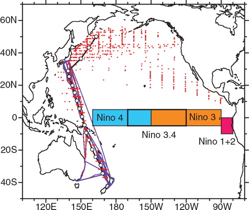
We have been conducting flask sampling for atmospheric O₂ and CO₂ in the northern and western Pacific regions since December 2001 (Tohjima et al., 2005b, 2012). Air samples have been collected on board VOSs travel routes between Japan and Australia/New Zealand (hereinafter referred to as the Oceanian route) and between Japan and the United States (hereinafter referred to as the North American route). In this study, we used the APO data obtained from the air samples collected until December 2012. The flask sampling locations are plotted in Fig. 1. The air samples on the Oceanian route were collected relatively regularly: usually 21 flasks during each 6-week round trip (7 and 14 flasks for southbound and northbound trip, respectively). Unfortunately, the sampling locations on the North American route were considerably scattered, because the ship tracks varied depending on the weather conditions and the destinations. Therefore, the flask data located to the north of 30°N cannot be interpreted as time series data.

Fig. 1 Locations where the O₂/N₂ ratios and CO₂ mixing ratios were observed. Red dots and purple lines indicate flask sampling and in-situ measurement sites, respectively. Open circles represent the average positions of the binned flask data. The black line connecting the open circles depicts the latitudinal transect, along which the observed and modelled APO values are compared. Four tropical Pacific regions for Niño 1+2 (10–0°S, 90–80°W), Niño 3 (5°S–5°N, 150–90°W), Niño 3.4 (5°S–5°N, 170–120°W) and Niño 4 (5°S–5°N, 160°E–150°W) indices are also shown.

The flasks were sent back to our laboratory, and the O₂/N₂ ratio and CO₂ concentrations were determined by a gas chromatograph equipped with a thermal conductivity detector (GC/TCD) and a non-dispersive infrared analyzer (NDIR), respectively (Tohjima, 2000). We report changes in the atmospheric O₂ concentrations as relative deviations of the O₂/N₂ ratio from an arbitrary reference according to1 and the relative deviations are expressed in per meg units (Keeling and Shertz, 1992). A value of 4.8 per meg corresponds to one molecule in 1 million of air molecule, or mole fraction of 1 µmol mol⁻¹ (ppm). Using δ(O₂/N₂), we calculated APO according to2 where β represents the −O₂:CO₂ molar exchange ratio for the land biotic respiration and photosynthesis (β=1.10±0.05, Severinghaus, 1995), X_CO2 is the CO₂ mol fraction in ppm, S_O2 is the atmospheric O₂ mole fraction in dry air (S_O2 =0.2094, Tohjima et al., 2005a), and 1850 is an arbitrary APO reference point. Note that δAPO is also expressed in per meg units. δ(O₂/N₂) values and CO₂ mole fractions were determined against the NIES O₂/N₂ scale (Tohjima et al., 2008) and the NIES 09 CO₂ scale (Machida et al., 2011), respectively.

2.2. Onboard in-situ measurements

In this study, we also employed atmospheric O₂/N₂ and CO₂ obtained from in-situ measurements taken on the Oceanian route during the period September 2007 to December 2012. The GC/TCD instrument was also used for the in-situ O₂/N₂ measurements. The detail of the onboard measurements of the O₂/N₂ ratio has already been presented elsewhere (Yamagishi et al., 2012). Although the onboard O₂/N₂ and CO₂ measurements are generally carried out at all times during the voyage, the data contaminated by the engine exhaust and urban emissions, which are easily distinguished by the short-term variability of CO₂, were not used in the study.

Comparing the onboard measurements with the flask data, the onboard in-situ O₂/N₂ values observed between June and July 2008 were found to be systematically higher than those of the flask data. Unfortunately, the reason for the discrepancy, which could be related to clogging of a filter and cold trap, is not fully understood. The O₂/N₂ measurements are easily biased by changes in the environmental conditions including temperature and pressure (Keeling et al., 1998a), and the analytical environment onboard the VOS is far from an ideal condition that exists in our laboratory. In addition, the reference gases used onboard the VOS have larger uncertainties in the O₂/N₂ values than those used in our laboratory, as described below. These facts have led us to conclude that the flask data are more accurate than the onboard in-situ data, but the onboard in-situ measurements give us a better spatiotemporal resolution than the flask measurements. The excursing in-situ O₂/N₂ data, therefore, were reduced by the average difference between the in-situ and flask data (20.5 per meg). After this ‘correction’, the average and standard deviation of the differences in δAPO between the in-situ (3-hour average) and flask measurements for the entire dataset reduced to −0.6±9.1 per meg. Although the average difference appears to suggest a general agreement between the in-situ and flask measurements, annual averages of the APO difference show a time-dependent variation with a range of −3.3 to 1.3 per meg. This time-dependent discrepancy suggests that the O₂/N₂ measurements were biased during the sampling and measurement procedures. The most plausible cause could be the uncertainty in the O₂/N₂ value for the reference gases used onboard the ship, which were usually replaced every 6 months. The O₂/N₂ values of the reference gases were calibrated against the NIES scale in our laboratory before and after every onboard use. Among these nine reference gases, the two reference gases showed about 9 per meg changes between before and after calibration, while the other differences were within 3 per meg. In this study, the O₂/N₂ values of these drifting standard gases during the onboard uses were linearly interpolated. Although this might suggest some difficulties in determining trends, Hamme and Keeling (2008) pointed out that the spatial gradient of APO is considered to be relatively unaffected by sampling and reference gas biases, allowing us to investigate the interannual variability in the distribution of the annual mean APO.

3. Model simulation

In order to examine how the year-to-year variation in the meteorological condition can influence the spatial gradient of the annual mean APO, we simulated APO by using an atmospheric tracer transport model driven by estimated surface O₂, N₂ and CO₂ fluxes. The model and the fluxes were basically the same as those used in Tohjima et al. (2012). For both oceanic O₂ and N₂ fluxes, climatological monthly anomalies [Garcia and Keeling (2001) for O₂ and Blaine (2005) for N₂] and annual mean fluxes [Gruber et al. (2001) for O₂ and Gloor et al. (2001) for N₂] were used. The spatial patterns of the annual mean O₂ and N₂ fluxes within the inversion boundaries were scaled to the spatial pattern of the annual mean heat flux estimated by Esbensen and Kushnir (1981). Tohjima et al. (2012) used monthly climatological sea surface CO₂ fluxes of Takahashi et al. (2002) and Takahashi et al. (2009), and showed that the latter ocean CO₂ flux reproduced better gradients of the observed annual mean APO, especially in the Southern Hemisphere. Therefore, in this study, we used the Takahashi et al. (2009) ocean CO₂ flux to drive the model. For global fossil fuel-derived CO₂ emissions, we used the 2006 values taken from the CDIAC database (Boden et al., 2011).

A NIES transport model ver. 99 (NIES99 TM, Maksyutov and Inoue, 2000), with 15 layers and 2.5°×2.5° horizontal resolution, was driven by the 12-hourly reanalysis meteorological data provided by the Japan Meteorological Agency (JMA) Climate Data Assimilation System (JCDAS) (Onogi et al., 2007). Separate simulation was run for each of the O₂, N₂ and CO₂ fluxes for the period 2001–2011. The 2001 meteorological data were used to spin up the model for 5 yr to achieve stable latitudinal gradients and other spatial patterns. APO values in per meg units were computed from the simulated O₂, N₂ and CO₂ mole fractions expressed in ppm according to the following equation:3 where the superscripts AM, SA, FF and OC denote the annual mean oceanic O₂ and N₂ fluxes, the seasonal anomaly of the oceanic O₂ and N₂ fluxes, the fossil fuel O₂ and CO₂ fluxes and the oceanic CO₂ fluxes, respectively, and S_N2 is the atmospheric N₂ mole fraction in dry air [S_N2 =0.7809 (Tohjima et al., 2005a)]. Following Tohjima et al. (2012), we refer to the first, second, third and fourth terms on the right hand side of eq. (3) as APO^AM, APO^SA, APO^FF and APO^OC components, respectively. As both the flask and onboard in-situ data were binned into about 10- and 1-degree latitudinal bands (see Section 4.1), we used the simulated APO for the average locations of the binned data with the daily intervals. Our previous study showed that the annual mean values based on the above simulated APO differed little from those based on simulated APO data, which were prepared by sampling the model output at the same locations and at the same time as the individual flask samples (Tohjima et al., 2012).

4. Results and discussion

4.1. Observed APO in the western Pacific

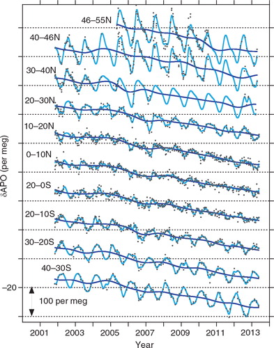
The APO data from flask samples were binned into 17 latitude bands of 40–30°S, 35–25°S, …, 40–46°N, and 46–55°N, as was done in Tohjima et al. (2012). However, in this study, we did not use the APO data to the east of longitude 180°E because these eastern data were not collected regularly in time and space. The average positions of the individual bins are shown in Fig. 1. The time series of the binned data are plotted in Fig. 2, together with smooth-curve fits to the data and trend curves that were computed by a time series analysis technique based on a least squares fitting and a low-pass digital filtering (Thoning et al., 1989). Note that we do not discuss interannual variations in the APO distribution to the north of 30°N because there were many data blank periods in the time series, for the reasons that were given in Section 2. We calculated the annual mean values of APO for the individual latitudinal bins from the corresponding smooth-curve fits.

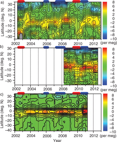
Fig. 2 Time series of APO based on the O₂/N₂ and CO₂ flask measurements. Light blue lines indicate the smooth-curve fits to the data, and the darker blue lines indicate the trend curves. The horizontal lines correspond to −20 per meg for the crossing time series. The distance between the horizontal lines is 100 per meg.

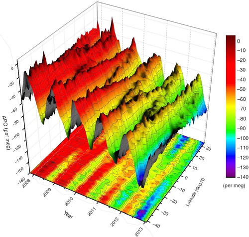
The APO data from the onboard in-situ measurements were binned into 1-degree latitude bands, and then smooth-curve fits to the individual binned data were computed by applying the same time series analysis technique used for the flask data. Figure 3 shows a time-latitude surface of the monthly mean APO computed from the smooth-curve fits. It is quite clear that the in situ measurements give us much denser APO data than the flask measurements, allowing us to examine much finer spatio-temporal variations in APO. The annual mean APO for each 1-degree latitude bin was calculated from the smooth-curve fits.

Fig. 3 Time-latitude surface depiction of monthly mean APO based on the in-situ measurements of atmospheric O₂ and CO₂ (Yamagishi et al., 2012) onboard VOS (TF5). The monthly means are computed for 1-degree latitude bands from the smooth curve fit to the binned data.

4.2. Latitudinal distribution of the annual mean APO

Figure 4a and 4b show the latitudinal distribution of the annual mean APO along the latitudinal transect based on the flask and in-situ measurements, respectively. To highlight the temporal changes in the latitudinal gradient, we detrended the annual mean APO in the individual bins by subtracting the average trends from both the flask and in-situ bins from 40°S to 30°N. In the figures, grey thick lines represent the average latitudinal distributions for the entire observation periods and the other lines represent the individual annual mean distributions centred on the date described in the legends. The latitudinal distributions based on the in-situ measurements were latitudinally smoothed by applying a five-degree moving average. As previously reported (Tohjima et al., 2012), the average latitudinal distributions clearly show the equatorial peaks and the mid-latitude troughs in the Northern Hemisphere. The average latitudinal distributions based on the in-situ measurements have fine latitudinal resolution and show general agreement with those based on the flask measurements. Upon closer examination, we find that the equatorial maximum of the average latitudinal distribution is located slightly to the south of the equator, at about 5°S. This APO maximum position may be explained by the distributions of the net O₂ and CO₂ emissions in the tropical Pacific and the atmospheric transport. The average latitudinal distribution of the simulated APO also shows a maximum at 5–2.5°S (see Fig. 4c), while the top portion of the simulated peak seems to be broader than the observation. But it is beyond the scope of this study to discuss these distributions in detail.

Fig. 4 Latitudinal distribution of the detrended annual mean APO based on the (a) flask measurements, (b) onboard in-situ measurements and (c) model simulations. The distributions are plotted along the latitudinal transect shown in Fig. 1. The black thick line in each panel represents an average distribution of all the values shown by the coloured lines. The red lines correspond to the distributions for the 2009/2010 El Niño period. The data labels (1 January 2003, etc.) indicate the centre of the averaging interval.

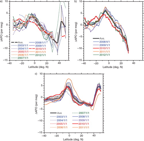
The equatorial bulges appeared to exist over much of the observation period. However, the latitudinal distributions centred on 1 January 2003 and 1 January 2010 were substantially suppressed, and were noticeably so in the Southern Hemisphere. There are slight differences in the suppressed latitudinal distribution for 1 January 2010 between the flask and in situ measurements; the flask measurements showed negative equatorward gradients in the annual mean APO in the Southern Hemisphere while the in situ measurements still showed slight equatorial elevations. In the Northern Hemisphere, on the other hand, the persistent presence of the deep decline in the annual mean APO between the equator and the mid-latitude (~40°N) makes the detectability of interannual variations in the latitudinal gradient difficult.

Time-latitude plots of the detrended annual mean APO based on the flask and in situ measurements are shown in Fig. 5a and 5b, respectively. For comparison, we also depict the periods of El Niño and La Niña events as red and blue bars, respectively, on the top of the figures. These periods were determined based on the definition used by the JMA (Trenberth, 1997) and the Niño 3 index, which is the SST anomaly averaged over the rectangle region of 150–90°W and 5°N–5°S (see Fig. 1). Both figures show suppressed equatorial bulges and reduced latitudinal gradients in the Southern Hemisphere during the period from the end of 2009 to the beginning of 2010, corresponding to the 2009/2010 El Niño period. Also, a similar suppression of the equatorial peak seemed to have occurred during the 2002/2003 El Niño period, as shown in Fig. 5a. On the other hand, substantial equatorial peaks seem to occur during La Niña periods, but we cannot find a clear relationship between the amplitude of the equatorial peak and a La Niña event from these plots.

Fig. 5 Time-latitude plot of the detrended annual mean APO based on the (a) flask measurements, (b) onboard in-situ measurements and (c) model simulations. The El Niño and La Niña periods are depicted as red and blue bars, respectively, on the top of each panel.

4.3. Simulated APO distribution

A profile and a time-latitude plot of the simulated annual mean APO along the latitudinal transect are shown in Figs. 4c and 5c, respectively. The simulation result clearly shows the interannual variations in the APO distribution, which can be attributed solely to the interannual variations in the atmospheric transport since climatological or year-to-year constant ocean fluxes (O₂, CO₂ and N₂) were used in the model simulation. It's notable that the amplitudes of the equatorial peaks are suppressed during El Niño periods and enhanced during La Niña periods. These variations are related to the ENSO cycle, especially the fact that the suppression of the APO bulge during El Niño periods is consistent with the observed variations.

In order to examine the influence of different atmospheric circulations on the temporal variability of the APO distribution, we show global distributions of the simulated annual mean APO centred on January 1, 2010 corresponding to an El Niño period and January 1, 2011 corresponding to a La Niña period in Fig. 6a and 6b, respectively. The most remarkable difference in the APO distribution between these two ENSO periods is the location of the equatorial bulge in the Pacific region; the peak of the equatorial bulge is located in the eastern Pacific during the El Niño period while it is shifted to the western Pacific during the La Niña period. The difference appears to be due to weak and strong easterly trade winds during the El Niño and La Niña periods, respectively.

Fig. 6 Global distribution of annual mean simulations for (a, b) total APO, (c, d) APO^AM, (e, f) APO^SA and (g, h) APO^OC. The left and right panels show the annual means centred on January 1, 2010 (El Niño period) and January 1, 2011 (La Niña period), respectively.

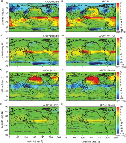
The global distributions of the APO components of APO^AM, APO^SA and APO^OC for the two different periods of the ENSO cycle are also depicted in Fig. 6c–h. Comparing the distributions of the APO components along the latitudinal transect for the El Niño period with those for the La Niña period, we find that the difference in the APO^AM distribution is considerably small. There is also little difference in the global distribution of APO^FF for the El Niño and La Niña periods (not shown). The largest contributor to the ENSO-related difference in the APO distribution along the latitudinal transect is APO^SA, with APO^OC as the next largest contributor. The annual mean APO^OC, reflecting the ocean CO₂ flux, has an equatorial bulge in the central Pacific region. The clearly identifiable area of the CO₂ bulge extends westward to the western Pacific during the La Niña period probably due to the strong easterly trade winds. On the other hand, the annual mean APO^SA generally shows an equatorial trough that is deep during the El Niño period and shallow during the La Niña period. This equatorial trough is attributed to the seasonal covariation (rectification) effect between the atmospheric transport and the seasonal ocean O₂ fluxes (Blaine, 2005; Tohjima et al., 2012). The variation in the seasonal rectification predominantly determines the observed spatio-temporal variation in APO. The equatorial region is predominantly influenced by the winter hemispheric air with relatively low APO values because the Intertropical Convergence Zone (ITCZ), shifting seasonally north and south, is generally located in the summer hemisphere. The annual mean position of the ITCZ, usually located to the north of the equator, moves toward and away from the equator during the El Niño and La Niña periods, respectively, especially in the western Pacific (Chen and Lin, 2005). Accordingly, the boreal winter air is more effectively transported to the equatorial region from the Northern Hemispheres during the El Niño period than during the La Niña period, causing lower annual mean APO in the equatorial region during the El Niño period in the model simulation.

Our simulations using the NIES99 model produced results that are in good agreement with the observed temporal variation in the tropical APO gradients, attributing about 80% of the variability in the equatorial Pacific bulge to the variability induced by the seasonal rectification, as discussed in the following section. However, since the TransCom APO experiments have shown a wide variation in the size and magnitude of the simulated rectifier effects of the tropical APO by various atmospheric transport models (Blaine, 2005), the true strength of the rectification is still not entirely settled. Since the equatorial seasonal rectification simulated by the NIES99 model was ‘middle-of-the-road’ in the TransCom APO experiments (Blaine, 2005), the model simulates a moderate seasonal rectification process relative to other atmospheric transport models, and we accept its ‘not-so-outrageous’ result of attributing much of the variations in the tropical APO gradient to the variability of the seasonal rectification.

4.4. Comparison of APO gradients

To quantify the temporal variations in the distribution of the annual mean APO in the Southern Hemisphere, we calculated latitudinal gradients between 25°S and the equator by using linear regression analysis. The temporal variations in the tropical APO gradients in the Southern Hemisphere for the observed and the simulated results are depicted in Fig. 7. The average gradient from the flask observation is less than half of those obtained from the in-situ and simulated values (Table 1); this is likely due to the rather coarser spatial resolution (10°) of the flask observation. The observed gradients show depleted values in 2002 and 2009/2010 and elevated values in 2003, 2008 and 2010/2012. The simulation captures the qualitative features of the observed variation, especially the substantial trough in 2009/2010, but the amplitude and phase of the APO variation are not necessarily well reproduced. However, the correlation coefficients between the observed and simulated APO gradients are greater than 0.6, with high significant levels (p<0.001) (Table 1).

Fig. 7 Temporal changes in the latitudinal gradient of the annual mean APO between 25°S and equator (left axis). Red and blue lines represent the flask and onboard in-situ measurements, respectively, and purple line represents the simulation. The time series of the Niño 4 index is also depicted at the bottom of the figure (right axis).

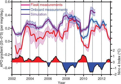
Table 1. Comparison of latitudinal APO gradients based on flask measurements, onboard measurements and model simulation

	Flask	Shipboard	NIES-TM
Time period	2002/5–2012/12	2008/4–2012/7	2001/1–2011/4
Average (±1σ)^a	0.12±0.12	0.25±0.10	0.26±0.09
Correlation coefficient^b	0.67 (<0.001)	0.81 (<0.001)
Variable ratio (±1σ)^c,d	0.73±0.05	0.79±0.08

^aValues are given in per meg/degree.

^bCorrelation coefficients of the measured and simulated APO time series for the overlapping periods are given. Values in parentheses are p-values.

^cVariable ratios are calculated as regression slopes of scatter plots of APO gradients between flask or shipboard observations (x-axis) and model simulations (y-axis) by using a reduced major axis (RMA) regression analysis (Hirsch and Gilroy, 1984).

^dUncertainties (±1σ) are computed by using bootstrap method.

To continue with the examination of the relationship between the APO gradients and the ENSO cycle, we also plot the Niño 4 index, which is based on the anomaly of SST in the Niño 4 region (5°S–5°N, 160°E–150°W) (data source: www.cpc.ncep.noaa.gov/data/indices/), in Fig. 7. The observed and simulated APO gradients seem to vary inversely with the Niño 4 Index. Table 2 summarises the correlation coefficients between the APO gradients and the four Niño indices: Niño 1+2 (10–0°S, 90–80°W), Niño 3, Niño 3.4 (5°S–5°N, 170–120°W) and Niño 4. The positive and negative anomalies of these indices correspond to the El Niño and La Niña conditions, respectively. Significant levels (p<0.05) of negative correlations are found between the observed APO gradients and the Niño 3, Niño 3.4 and Niño 4 indices, while there are no significant correlations between the observed APO gradients and the Niño 1+2 index. The absolute value of the correlation coefficient increases from Niño 1+2, Niño 3, Niño 3.4, to Niño 4, consistent with the fact that the shipboard observations were carried out in the western Pacific. The simulated APO gradients show greater correlations with the Niño indices than the observed gradients, while showing the same order of increasing correlation with various Niño indices.

Table 2. Correlation coefficients between the APO gradients and ENSO indices

	Flask		Shipboard		NIES-TM
ENSO indices	Zero-lag^a	Lagged^b	Zero-lag^a	Lagged^b	Zero-lag^a	Lagged^b
Nino 1+2	0.17 (0.06)	−0.34 (+10)	−0.03 (0.86)	−0.38 (+7)	−0.26 (0.01)	−0.51 (+3)
Nino 3	−0.28 (0.001)	−0.50 (+5)	−0.46 (<0.001)	−0.68 (+3)	−0.70 (<0.001)	−0.78 (+2)
Nino 3.4	−0.49 (<0.001)	−0.65 (+4)	−0.65 (<0.001)	−0.80 (+3)	−0.84 (<0.001)	−0.87 (+1)
Nino 4	−0.55 (<0.001)	−0.69 (+4)	−0.76 (<0.001)	−0.84 (+2)	−0.88 (<0.001)	−0.90 (+1)

^aValues in parentheses are p-values.

^bValues in parentheses are lag times (in months) which give the best correlation coefficients. Plus value means that the APO gradient lags behind the ENSO index.

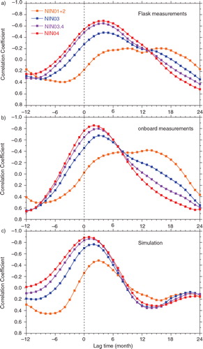
As can be seen in Fig. 7, the observed APO gradients seem to lag behind those of the Niño 4 index by a few months. We therefore calculated lagged correlation between the four Niño indices and the observed and simulated APO gradients (Fig. 8). Clearly, there is a general tendency for the maximum negative correlation to increase (in absolute magnitude) and for the lag time to decrease as one move westward. Table 2 lists the lag time (in months) when maximum negative correlation occurs. These results can be explained by the fact that the temporal variation in the western Niño index lags behind those of the eastern Niño index by a few to several months. It should be noted that the observed correlation with the Niño 1+2 index shows a plateaued relationship compared to the simulated correlation and the maximum negative values appear to occur with lags greater than 12 months. The Niño 1+2 index, reflecting the strength of the upwelling in the tropical eastern Pacific, is also indicative of the nutrient supply to the surface, which influences the level of biological production. The delayed response of the observed APO gradients to the Niño 1+2 index could be explained by the possibility that the subsequent biological O₂ emissions are delayed from the time of the upwelling by more than a typical El Nino duration (Rödenbeck et al., 2008). It is also worth noting that the observed lag for the maximum negative correlation is on the order of a few months longer than the simulated lags. The difference suggests the existence of temporal variations in the APO fluxes that correlate negatively with the ENSO indices with lag times of several months. The inferred flux variation seems consistent with the discussion in Section 4.5.

Fig. 8 Correlation coefficients between the Niño indices and the lagged APO gradients (25–0°S) based on the (a) flask measurements, (b) onboard in-situ measurements and (c) model simulation. Orange, blue, purple and red lines correspond to the Niño 1+2, Niño 3, Niño 3.4 and Niño 4 indices, respectively.

As discussed above, the model simulation reproduced the characteristics of the temporal variations in the observed APO gradients well in spite of the climatological and constant APO fluxes used in the simulations. However, the simulation slightly underestimated the temporal variations in comparison with the observations. The variable ratios of the simulated APO gradients to the observed APO gradients are less than 0.8 (Table 1). Therefore, 21–27% of the variability in the APO gradients (0.10–0.12 per meg/degree), which corresponds to about 0.03 per meg/degree, should be attributed to the inaccuracy in the variability in the oceanic fluxes of O₂ and CO₂ or in the model simulation of the tropical circulation.

4.5. Sensitivity of APO gradient to the tropical emissions

In order to evaluate the sensitivity of the simulated latitudinal APO gradient for 25–0°S to the oceanic fluxes of O₂ and CO₂ from the tropical Pacific, we conducted a set of perturbation experiments as follows: First, we modified the monthly oceanic CO₂ flux of Takahashi et al. (2009) and the annual oceanic O₂ flux map by scaling those fluxes from the tropical Pacific region by factors of 0, 0.5 and 1.5. The relative distribution of the fluxes within the tropical Pacific region (defined by 20°S–20°N and 120°E–80°W) was not changed in these simulations. These modified fluxes were then used to conduct two sets of model experiments, one using different O₂ flux values only, and the other one using different CO₂ fluxes only. All other variables were kept the same as in the previous simulation (Section 4.3). The relationship between the average APO gradients and the net O₂ and CO₂ emission from the tropical Pacific region are depicted in Fig. 9. The APO gradients, linearly changing with the O₂ and CO₂ emissions from the tropical Pacific regions, are more sensitive to the O₂ emissions than to the CO₂ emissions. The sensitivities of the APO gradients to the tropical O₂ and CO₂ emissions are 0.0030 (per meg/degree)/(Tmol O₂/yr) and 0.0013 (per meg/degree)/(Tmol C/yr), respectively. These different sensitivities are explained by the differences in the longitudinal emission distribution between O₂ and CO₂: the O₂ emission from the western half of the equatorial Pacific region contributes 54% of the total tropical Pacific emission (112 Tmol O₂/yr for normal case), while the CO₂ emission from the western half contributes only 6% of the total emission (0.46PgC/yr or 38 Tmol C/yr for normal case).

Fig. 9 Relationship between the simulated APO gradients (25–0°S) and the net O₂ and CO₂ emission from the tropical Pacific region (20°S–20°N and 120°E–80°W), obtained from the experimental simulations (see text). The APO gradients are the averages for the entire simulation period and the vertical bars represent the standard deviations (1σ). The broken lines are linear regression fits.

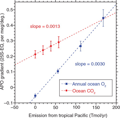
Using these sensitivities, the variations in the APO gradient can be converted to potential ocean O₂ or CO₂ flux variations. For example, the variability in the APO gradient of 0.03 per meg/degree, which is the amount of variability exceeding model prediction, as discussed in Section 4.4, corresponds to potential fluxes of ±10 Tmol O₂/yr or ±23 Tmol C/yr. Therefore, a model simulation driven by the additional O₂ or CO₂ flux variations with above amplitudes associated with outgassing during La Niña and ingassing during El Niño can reproduce the observed APO gradient variations.

The CO₂ flux from the tropical Pacific estimated from extensive ocean CO₂ partial-pressure (pCO₂) measurements showed significant decrease and increase during the El Niño and La Niña events, respectively, with a variability ranging from ±10 to ±20 Tmol C/yr (Feely et al., 2006). These variations in the ocean CO₂ flux are relatively consistent with the above-mentioned potential APO flux variability in amplitude and its relationship to the ENSO cycle. The ocean biological O₂ fluxes are also estimated to have similar ENSO-related variations. Satellite colour measurements have revealed that the ocean net primary production (NPP) can vary inversely with SST anomaly and that the NPP in the low latitude band from 40°S to 40°N can have ENSO related variations, suppressing NPP during an El Niño period, with the variability on the order ±100 Tmol C/yr (Behrenfeld et al., 2006). The net O₂ flux affecting the APO variation is related to the net ecosystem production (NEP). In the open ocean, the NEP/NPP ratio is estimated to 0.1–0.2 (Laws et al., 2000). Therefore, assuming that the NPP variability in the Pacific Ocean contributes about half of the global NPP variability, we obtain a biotic O₂ flux variability on the order of ±5 to ±10 Tmol C/yr. This O₂ flux variability is also roughly consistent with the above-mentioned potential APO flux variability in magnitude and its relationship to the ENSO cycle.

On the other hand, an inversion study based on the APO dataset from the Scripps network (Rödenbeck et al., 2008) showed that the APO outgassing fluxes in the tropical Pacific (20°S–20°N) increases during El Niño and decreases during La Niña, with a variability of about ±50 Tmol O₂/yr. Given the sensitivities to the tropical O₂ or CO₂ fluxes already discussed above, the inversion-based APO flux variations cause increase and decrease in the latitudinal APO gradients during El Niño and La Niña, respectively, with the amplitude of ±0.07 to ±0.15 per meg/degree. Such variations could have considerably suppressed the observed variations presented in this study.

It has been argued that atmospheric O₂ is taken up by the ocean at mid- to high-latitudes, transported equatorward by the large-scale ocean circulation and again emitted to the atmosphere at low latitudes (cf. Keeling et al., 1993; Gruber et al., 2001). The air–sea CO₂ exchanges in general show similar latitudinal contrast as O₂ (cf. Takahashi et al., 2009). It is therefore logical that a strengthening of the equatorial upwelling along the equator in the eastern Pacific would enhance the tropical APO outgassing fluxes, and vice versa. This reasoning is consistent with our results.

The seemingly inconsistent results of Rödenbeck et al. (2008) and this study can be made more compatible by considering that the tropical APO gradient of this study is more sensitive to the emissions from the western Pacific than those from the eastern Pacific. The influence of the O₂ flux variations in the upwelling regions on the APO gradients could be offset by smaller antiphase O₂ flux variations in the western Pacific. If that is the case, the APO outgassing fluxes in the western Pacific vary with the ENSO cycle, decreasing (increasing) during El Niño (La Niña) periods. To resolve the zonal differences in the APO flux variations in the tropical Pacific, therefore, a new inversion study using adequate tropical Pacific APO observations, including ours, and improved atmospheric transport models would be required.

5. Conclusion

We have examined the temporal variation in the latitudinal distribution of annual mean APO based on flask samples and in-situ measurements onboard VOSs sailing in the western Pacific, mainly between Japan and Australia/New Zealand (40°S to 30°N). Although most of the latitudinal distributions of the annual mean APO clearly show equatorial bulges, a substantial suppression of the equatorial bulge was observed during the 2009/2010 El Niño period, especially in the Southern Hemisphere. We calculated latitudinal gradients of the annual mean APO between 25°S and equator by using a linear regression method, and then compared them with the Niño 1+2, 3, 3.4 and 4 indices. In order to evaluate the influence of the atmospheric transport on the APO distribution, we simulated APO by using the NIES atmospheric transport model (NIES99 TM) driven by a set of surface CO₂, O₂ and N₂ fluxes that were constant in time or varied with a monthly climatological cycle. We also compared the observed APO gradients with the simulated results. From these analyses and comparisons, we obtain the following conclusions:

1. The latitudinal gradients of the southern slope of the equatorial APO bulge show significant negative correlations with the Niño 3, 3.4 and 4 indices. This result indicates that the amplitude of the equatorial APO bulge varies with the ENSO cycle, being enhanced and suppressed during La Niña and El Niño, respectively. The variability in the latitudinal gradient is about ±0.1 per meg/degree, which corresponds to an amplitude of about ±3 per meg on the south side of the equatorial bulge.

2. The model simulation reproduces the temporal variations in the observed APO gradients well, suggesting that the atmospheric transport is the main contributor to the temporal variations in the global APO distribution. The observed ENSO-related variations in the equatorial bulge may be explained by the location of the equatorial area with elevated APO, which moves eastward (westward) during El Niño (La Niña) associated with the weak (strong) easterly trade wind.

3. The model simulation underestimates by about 25% the temporal variations in the APO gradients in comparison with the observation. This underestimation might suggest the existence of compensating tropical APO outgassing fluxes associated with the ENSO cycle: decrease during El Niño and increase during La Niña. Using the simulated sensitivities of the APO gradient to the O₂ or CO₂ fluxes from the tropical Pacific regions, we have estimated the variability of the compensating APO fluxes to be ±10 Tmol O₂/yr or ±23 Tmol C/yr. These fluxes are roughly consistent with the results from the pCO₂ observations (Feely et al., 2006) and the satellite measurements (Behrenfeld et al., 2006).

4. The inversion-based APO outgassing fluxes from the equatorial Pacific have been shown to increase (decrease) during El Niño (La Niña) (Rödenbeck et al., 2008), which appears to be inconsistent with our results. These seemingly inconsistent results could be resolved by taking into account the different sensitivities of the equatorial APO gradients to fluxes from different regions.

Our model analysis also suggests that much of the observed interannual variations in the tropical APO gradients are due to the tropical rectification. However, since this conclusion is based on the results from only one model, further studies on this subject involving multiple models are needed. In addition, previous inversion studies based on the observations from a limited number of fixed stations might have been poorly constrained to clearly identify the variation in the APO fluxes over the tropical Pacific regions. Including our shipboard observations would reduce the data-dependent uncertainty in the spatiotemporal resolution of the APO flux variability, leading to a better understanding of the ocean biogeochemical processes.

6. Acknowledgements

We gratefully acknowledge Shigeru Kariya, Tomoyasu Yamada and other members of the Global Environment Forum (GEF) for their continued support in maintaining the measurements of CO₂, and O₂/N₂ ratio onboard VOSs. Thanks are also expressed to the owners, operators and crew of the VOSs, MOL Golden Wattle, MOL Glory, Fujitrans World, Trans Future 5, Pyxis, and Skaubryn, for giving us the wonderful opportunity of the observations. We thank Yoko Kajita and Hisayo Sandanbata for the preparation and measurement of the flask samples, Keiichi Katsumata for preparing the CO₂ and O₂/N₂ reference gases, and Sumiko Harasawa and Chisato Wada for processing the onboard CO₂ data. The JCDAS data sets used for this study are provided by the cooperative research project of the JRA-25 long-term reanalysis by the Japan Meteorological Agency (JMA) and the Central Research Institute of Electric Power Industry (CRIEPI). Two anonymous reviewers made valuable comments, which helped to improve the manuscript considerably. This work has been financially supported by the Ministry of the Environment through the Global Environment Research Account for National Institutes (E0450 and E0955).

References

- Balkanski Y. , Monfray P. , Battle M. , Heimann M . Ocean primary production derived from satellite data: an evaluation with atmospheric oxygen measurements. Glob. Biogeochem. Cycles. 1999; 13: 257–271.
- Battle M. , Bender M. L. , Tans P. P. , White J. W. C. , Ellis J. T. , co-authors . Global carbon sinks and their variability inferred from atmospheric O2 and δ13C. Science. 2000; 287: 2467–2470.
- Battle M. , Fletcher S. M. , Bender M. L. , Keeling R. F. , Manning A. C. , co-authors . Atmospheric potential oxygen: new observations and their implications for some atmospheric and oceanic models. Glob. Biogeochem. Cycles. 2006; 20: 1010.
- Behrenfeld M. J. , O'Malley R. T. , Siegel D. A. , McClain C. R. , Sarmiento J. L. , co-authors . Climate-driven trends in contemporary ocean productivity. Nature. 2006; 444: 752–755.
- Bender M. , Ellis T. , Tans P. , Francey R. , Lowe D . Variability in the O2/N2 ratio of southern hemisphere air, 1991–1994: implications for the carbon cycle. Glob. Biogeochem. Cycles. 1996; 10: 9–21.
- Bender M. L. , Ho D. T. , Hendricks M. B. , Mika R. , Battle M. O. , co-authors . Atmospheric O2/N2 changes, 1993–2002: implications for the partitioning of fossil fuel CO2 sequestration. Glob. Biogeochem. Cycles. 2005; 19: 4017.
- Blaine T. W . Continuous Measurements of Atmospheric Ar/N2 as a Tracer of Air-Sea Heat Flux: Models, Methods, and Data.
- Boden T. A. , Marland G. , Andres R. J . Global, Regional, and National Fossil-Fuel CO2 Emissions. 2011. Carbon Dioxide Information Analysis Center, Oak Ridge National Laboratory, U.S. Department of Energy, Oak Ridge, TN. DOI: 10.3334/CDIAC/00001_V2011.
- Chen G. , Lin H . Impact of El Nino/La Nina on the seasonality of oceanic water vapor: a proposed scheme for determining the ITCZ. Mon. Weather Rev. 2005; 133: 2940–2946.
- Esbensen S. K. , Kushnir J . The Heat Budget of the Global Ocean: An Atlas Based on Estimates from Marine Surface Observations. 1981; Oregon State University, Corvallis, OR: Climate Research Institute. Report No. 29.
- Feely R. A. , Takahashi T. , Wanninkhof R. , McPhaden M. J. , Cosca C. E. , co-authors . Decadal variability of the air–sea CO2 fluxes in the equatorial Pacific Ocean. J. Geophys. Res. 2006; 111: 08S90.
- Garcia H. E. , Keeling R. F . On the global oxygen anomaly and air–sea flux. J. Geophys. Res. 2001; 106: 31155–31166.
- Gloor M. , Gruber N. , Hughes T. M. , Sarmiento J. L . An inverse modeling method for estimation of net air–sea fluxes from bulk data: methodology and application to the heat cycle. Glob. Biogeochem. Cycles. 2001; 15: 767–782.
- Gruber N. , Gloor M. , Fan S.-M. , Sarmiento J. L . Air–sea flux of oxygen estimated from bulk data: implications for the marine and atmospheric oxygen. Glob. Biogeochem. Cycles. 2001; 15: 783–803.
- Hamme R. C. , Keeling R. F . Ocean ventilation as a driver of interannual variability in atmospheric potential oxygen. Tellus B. 2008; 60: 706–717.
- Hirsch R. M. , Gilroy E. J . Methods of fitting a straight line to data: examples in water resources. Water Resour. Bull. 1984; 20: 705–711.
- Keeling R. F. , Najjar R. P. , Bender M. L. , Tans P. P . What atmospheric oxygen measurements can tell us about the global carbon cycle. Glob. Biogeochem. Cycles. 1993; 7: 37–67.
- Keeling R. F. , Shertz S. R . Seasonal and interannual variations in atmospheric oxygen and implications for the global carbon cycle. Nature. 1992; 358: 723–727.
- Keeling R. F. , Stephens B. B. , Najjar R. G. , Doney S. C. , Archer D. , co-authors . Seasonal variation in the atmospheric O2/N2 ratio in relation to the kinetics of air–sea gas exchange. Glob. Biogeochem. Cycles. 1998b; 12: 141–163.
- Keeling R. R. , Manning A. C. , McEvoy E. M. , Shertz S. R . Method for measuring changes in atmospheric O2 concentration and their application in southern hemisphere air. J. Geophys. Res. 1998a; 103: 3381–3397.
- Laws E. A. , Falkowski P. G. , Smith W. O. Jr. , Ducklow H. , McCarthy J. J . Temperature effects on export production in the open ocean. Glob. Biogeochem. Cycles. 2000; 14: 1231–1246.
- Machida T. , Tohjima Y. , Katsumata K. , Mukai H . Brand W. A . A new CO2 calibration scale based on gravimetric one-step dilution cylinders in National Institute for Environmental Studies-NIES 09 CO2 scale. Report of the 15th WMO Meeting of Experts on Carbon Dioxide Concentration and Related Tracer Measurement Techniques. 2011; Switzerland: Geneva. 114–118. Jena, Germany, September 7–10, 2009, WMO/GAW Report No. 194, WMO.
- Maksyutov S. , Inoue G . Shimizu H . Vertical profiles of radon and CO2 simulated by the global atmospheric transport mode. CGER Supercomputer Activity Report, 1039–2000, 7. 2000; Tsukuba, Japan: CGER NIES. 39–41.
- Manning A. C. , Keeling R. F . Global oceanic and biotic carbon sinks from the Scripps atmospheric oxygen flask sampling network. Tellus B. 2006; 58: 95–116.
- Naegler T. , Ciais P. , Orr J. C. , Aumont O. , Rödenbeck C . On evaluating ocean models with atmospheric potential oxygen. Tellus B. 2007; 59: 138–156.
- Nevison C. C., Mahowald N. M., Doney S. C., Lima I. D., Cassar N. Impact of variable air–sea O2 and CO2 fluxes on atmospheric potential oxygen (APO) and land–ocean carbon sink partitioning. Biogeosciences. 2008; 5: 875–889. www.biogeosciences.net/5/875/2008/.
- Onogi K. , Tsutsui J. , Koide H. , Sakamoto M. , Kobayashi S. , co-authors . The JRA-25 Reanalysis. J. Meteorol. Soc. Jpn. 2007; 85: 369–432.
- Rödenbeck C. , Le Quéré C. , Heimann M. , Keeling R. F . Interannual variability inoceanic biogeochemical processes inferred by inversion of atmospheric O2/N2 and CO2 data. Tellus B. 2008; 60: 685–705.
- Severinghaus J. P . Studies of the Terrestrial O2 and Carbon Cycles in Sand Dune Gases and in Biosphere 2.
- Stephens B. B. , Keeling R. F. , Heimann M. , Six K. D. , Murnane R. , co-authors . Testing global ocean carbon cycle models using measurements of atmospheric O2 and CO2 concentration. Glob. Biogeochem. Cycles. 1998; 12: 213–230.
- Takahashi T. , Sutherland S. C. , Sweeney C. , Poisson A. , Metzl N. , co-authors . Global sea–air CO2 flux based on climatological surface ocean pCO2, and seasonal biological and temperature effects. Deep Sea Res. II. 2002; 49: 1601–1622.
- Takahashi T. , Sutherland S. C. , Wanninkhof R. , Sweeney C. , Feely R. A. , co-authors . Climatological mean and decadal change in surface ocean pCO2, and net sea–air CO2 flux over the global oceans. Deep Sea Res. II. 2009; 56: 554–577.
- Thoning K.W. , Tans P. P. , Komhyr W. D . Atmospheric carbon dioxide at Mauna Loa Observatory 2. Analysis of the NOAA GMCC data, 1974–1985. J. Geophys. Res. 1989; 94: 8549–8565.
- Tohjima Y . Method for measuring changes in the atmospheric O2/N2 ratio by a gas chromatograph equipped with a thermal conductivity detector. J. Geophys. Res. 2000; 105: 14575–14584.
- Tohjima Y. , Machida T. , Watai T. , Akama I. , Amari T. , co-authors . Preparation of gravimetric standards for measurements of atmospheric oxygen and re-evaluation of atmospheric oxygen concentration. J. Geophys. Res. 2005a; 110: 11302.
- Tohjima Y. , Minejima C. , Mukai H. , Machida T. , Yamagishi H. , co-authors . Analysis of seasonality and annual mean distribution of atmospheric potential oxygen (APO) in the Pacific region. Glob. Biogeochem. Cycles. 2012; 26: 4008.
- Tohjima Y. , Mukai H. , Machida T. , Nojiri Y. , Gloor M . First measurements of the latitudinal atmospheric O2 and CO2 distributions across the western Pacific. Geophys. Res. Lett. 2005b; 32: 17805.
- Tohjima Y. , Mukai H. , Nojiri Y. , Yamagishi H. , Machida T . Atmospheric O2/N2 measurements at two Japanese sites: estimation of global oceanic and land biotic carbon sinks and analysis of the variations in atmospheric potential oxygen (APO). Tellus B. 2008; 60: 213–225.
- Trenberth K. E . The definition of El Nino. Bull. Am. Meteorol. Soc. 1997; 78: 2771–2777.
- Yamagishi H. , Tohjima Y. , Mukai H. , Nojiri Y. , Miyazaki C. , co-authors . Observation of atmospheric oxygen/nitrogen ratio aboard a cargo ship using gas chromatography/thermal conductivity detector. J. Geophys. Res. 2012; 117: 04309.