Methane exchange in a boreal forest estimated by gradient method

Abstract

Forests are generally considered to be net sinks of atmospheric methane (CH₄) because of oxidation by methanotrophic bacteria in well-aerated forests soils. However, emissions from wet forest soils, and sometimes canopy fluxes, are often neglected when quantifying the CH₄ budget of a forest. We used a modified Bowen ratio method and combined eddy covariance and gradient methods to estimate net CH₄ exchange at a boreal forest site in central Sweden. Results indicate that the site is a net source of CH₄. This is in contrast to soil, branch and leaf chamber measurements of uptake of CH₄. Wetter soils within the footprint of the canopy are thought to be responsible for the discrepancy. We found no evidence for canopy emissions per se. However, the diel pattern of the CH₄ exchange with minimum emissions at daytime correlated well with gross primary production, which supports an uptake in the canopy. More distant source areas could also contribute to the diel pattern; their contribution might be greater at night during stable boundary layer conditions.

• micrometeorology
• Bowen ratio
• eddy covariance
• footprint
• wet soil

1. Introduction

Forests cover about 30% of the world's land surface area and they can host both methane (CH₄) consuming (Harriss et al., 1982) and CH₄ emitting (Ehhalt, 1974) soil environments. A well-aerated forest soil is a net sink of atmospheric CH₄, thanks to oxidation by methanotrophic bacteria (Born et al., 1990; Whalen and Reeburgh, 1990; Crill, 1991). However, this does not necessarily mean that forests are always a net sink of CH₄. Production of CH₄, by archaea, takes place in anoxic environments such as water-saturated soils and small ponds scattered in forests and in anaerobic micro sites within otherwise well-drained soils (Hudgens and Yavitt, 1997; Von Fischer and Hedin, 2002; Kammann et al., 2009). It is possible that the CH₄ uptake rate in forests, especially in moist forests, is overestimated since emissions from wet soils are not adequately accounted for (Grunwald et al., 2012). Even if CH₄ emissions are sporadic and limited to restricted areas, their occurrence frequency and source strength might turn a forest from a net sink to a net source of CH₄ (Fiedler et al., 2005; Sakabe et al., 2012). The capacity of plants with roots in CH₄-rich water-saturated soils, even woody plants, to transport and release CH₄ (Terazawa et al., 2007; Gauci et al., 2010) adds another level of the complexity to the analyses.

Soil moisture, soil texture and water table depth are crucial in determining whether the soil will act as a net CH₄ sink or CH₄ source. Soil moisture and soil texture influence the soil diffusivity and thus the flux of CH₄ and oxygen from the atmosphere to the soil depths where CH₄ is consumed (Born et al., 1990; Koschorreck and Conrad, 1993; Whalen and Reeburgh, 1996), while water table depth alters the relative extent of anaerobic and aerobic zones in the soil (Whalen and Reeburgh, 1990). Soil moisture and water table depth vary spatially due to, for example, topography, which results in spatial variations of CH₄ exchange (Lessard et al., 1994; Yu K. W. et al., 2008). There is also a temporal variability in CH₄ exchange, mainly due to changes in temperatures and precipitation (Castro et al., 1994; Guckland et al., 2009). CH₄ production is strongly favoured by increasing temperatures, while CH₄ oxidation is not as sensitive to temperature changes (Dunfield et al., 1993; Yvon-Durocher et al., 2014). Soils have been observed to switch from sinks to sources following precipitation (Keller and Reiners 1994; Wang F. L. and Bettany 1995; Hudgens and Yavitt 1997; Sakabe et al., 2012).

To date, most in situ measurements of CH₄ have been made with chambers (e.g., Crill et al., 1994; Bradford et al., 2000; Guckland et al., 2009). They are suitable for detailed studies of processes controlling CH₄ exchange, but they might not be spatially representative for a larger area (Denmead, 2008), and semi-continuous measurements are only possible with automated chambers. Micrometeorological (MM) methods, such as gradient methods and eddy covariance (EC) methods, can better capture spatial and temporal variability of CH₄ exchange over forests at hectare or larger scales. Net ecosystem carbon dioxide (CO₂) exchange between forests and the lower atmosphere has been measured with gradients since 1970 and with EC since the early 1990s (Baldocchi et al., 2001). Measuring CH₄ exchange is more challenging than measuring CO₂ exchange due to low flux rates from spatially restricted areas within a forest and therefore relatively few MM studies exist to date (Nicolini 2013). CH₄ exchange between forest stands and the atmosphere has been measured by EC (Smeets et al., 2009; Shoemaker et al., 2014), relaxed EC (Sakabe et al., 2012; Ueyama et al., 2012), and by gradient methods (Simpson et al., 1997; Bowling et al., 2009; Querino et al., 2011).

For the present study, we used a gradient method to analyse CH₄ exchange at a boreal forest site in central Sweden. The aim was to quantify the CH₄ exchange between the soil surface and the overlying atmosphere and to investigate the reasons for variability of CH₄ exchange over time. We further compared the result from MM methods with soil chamber measurements from within the spatial and temporal footprint of the former. The rationale for choosing the gradient method instead of the nowadays more common EC method was that we believed that the small fluxes to be expected from the forest could be more accurately estimated with the gradient method than with the EC method. With a high tower, large vertical separation between the CH₄ intakes can be achieved which thus maximises the concentration differences while the high frequency concentration measurements in the EC method would be hampered by the analyser noise, which would be larger than the expected CH₄ fluctuations. The Norunda forest represents a typical hemi-boreal forest consisting of a mixture of pine and spruce trees.

2. Method

2.1. Site description

The CH₄ gradient measurements were made at the Norunda research station, a boreal forest site, 60°5′N, 17°29′E in central Sweden, from 16 June 2010 to 31 December 2011. A forest stand consisting of 120-year-old mixed pine (Pinus sylvestris) and spruce (Picea abies) trees surrounded the measurement tower within a 500 m radius. The forest in the south-west (SW) to north-east (NE) directions had not been thinned or fertilised in a few decades, while NE to SW quadrants were thinned in 2008 which decreased the leaf area index in average from 4.8 to 2.8 m² m⁻². Forest stands of various ages covered most of the area within a 500–800 m radius around the tower, apart from a clear-cut area of 6.5 ha in the west and a smaller clear-cut area in the south. Tree heights at the site were generally around 25 m. At distances greater than 800 m, agricultural lands, wetlands and lakes contributed to the mosaic of the landscape (Fig. 1).

Fig. 1 Digital surface model (DSM) of the Norunda site. The circles denote 500 m (orange) and 800 m (yellow) distance from the tower (red dot).

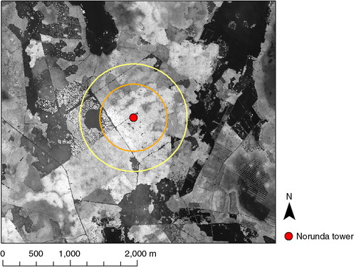
Understory vegetation at the site was sparse and dominated by bilberry (Vaccinium myrtillus) and feathermosses (Hylocomium splendens and Pleurozium schreberi). The soil was a glacial till (Lundin et al., 1999) with an organic layer of 3–10 cm depth.

2.2. Instrumentation

Concentrations of CH₄ and CO₂ were measured at three heights (31.7, 58.5 and 100.6 m) above ground, with an off-axis integrated cavity output spectroscopic (ICOS) laser analyser (DLT-100, Los Gatos Research (LGR)). All intakes were above the canopy. The 31.7 m intake was located within the roughness sublayer, while the other two intakes were in the semi-logarithmic layer. Displacement height was estimated to be 21.1 m (Mölder et al., 1999).

Air was pulled to the analyser through 4 mm high-density polyethene tubing. An individual membrane pump was used for each level and all lines were flushed continuously and also at the same flow rate during sub-sampling of air to the gas analyser. An 8 L mixing volume was installed at the inlet of each line, and a perma pure dryer was used to dry the air before the analyser. Each level was sampled for 5 min. The gas analyser was measured at a frequency of 1 Hz. The flow rate through the tubing was set to 3 L min⁻¹, and the sub-sampling rate through the analyser was 0.7 L min⁻¹. The excess flow was vented through a T-connector.

EC measurements of CO₂ exchange were conducted at 33 m height with a 3-D sonic anemometer (USA-1, Metek GmbH) and an infrared gas analyser (LI-7000, Li-Cor, Inc.). The air was drawn to the gas analyser through 6 m of 4 mm high-density polyethene tubing at a rate of 8–9 L min⁻¹. Turbulence and concentration were measured at 10 Hz, and fluxes were calculated as 30-min averages. Linear detrending was used, and the time lag between wind and gas concentration measurements was determined by maximum correlation. No frequency correction due to tube dampening was done as the correction is negligible for the current set-up with relatively short intake tube and high flow rate as well as high measurement height above ground.

Chamber measurements were made 100 m to the NW of the tower from 7 July 2010 to 4 October 2010 (Sundqvist et al., 2014). We used five automated, transparent chambers of polymethyl methacrylate, which each covered a surface area of 0.2 m² and had a total volume of 110 L. In accordance with the tower measurements, chamber CH₄ concentrations were measured with an ICOS laser gas-analyser (DLT-100, LGR) that was located at a minimum of 4 m and a maximum of 15 m from the chambers. During the 6 min of each measurement, the chambers were closed and air was recirculated through the gas analyser. A fan was installed in each chamber to ensure sufficient mixing of the chamber headspace air. The fan was carefully adjusted to avoid disturbing the boundary layer at the soil surface. Chamber frames were installed at a depth of about 3 cm in 2005; so by 2010, there had been sufficient time for soil and vegetation to recover from the disturbance.

Continuous measurements of soil temperature, air temperature, precipitation, water table depth and soil moisture were made and stored at 10 s intervals. Air temperature was measured at 32 m height on the tower with a type T thermocouple placed in a ventilated radiation shield. Soil temperature was measured near the tower at 10 cm depth with a type T thermocouple. Soil moisture was measured at 20 cm depth with permittivity sensors (Ml-2x ThetaProbe, Delta-T Devices Ltd). Precipitation was measured using a tipping bucket rain gauge (RM Young Company), at an open site 80 m E of the tower. Water table depth was measured 80 m N of the tower.

2.3. Gradient methods

CH₄ exchange was calculated using two different methods, a modified Bowen ratio (BR) method and a combined EC and gradient method (ECG). CH₄ exchange was calculated from gradients between 31.7 and 58.5 m height and from gradients between 31.7 and 100.6 m height. In the following, fluxes calculated by the modified BR method using gradients between 31.7 and 58.5 m will be referred to as BR1. BR2 will be used when the fluxes are based on gradients between 31.7 and 100.6 m. Similarly, fluxes calculated by the ECG method will be referred to as ECG1 and ECG2 (gradients between 31.7 and 58.5 m and between 31.7 and 100.6 m, respectively).

The ECG method is described in detail by Denmead (2008) and Simpson et al. (1997), among others. Similar to Fick's law of diffusion, the vertical turbulent transport of CH₄ in the atmosphere is given by1

where V (m³ mol⁻¹) is the volume of 1 mol of air and C is the CH₄ concentration (µmol mol⁻¹). The turbulent diffusivity K _c, valid for a specific layer in the atmosphere, is derived from the Monin–Obukhov similarity theory,2

where k=0.4 is the von Karman constant, for u _* and 10 Wm⁻² for the (m s⁻¹) the friction velocity, z ₂(m) the upper air intake height, z ₁(m) is the lower air intake height, Δz is the difference between the intake heights, L is the Obukhov length and ψ _t the diabatic correction function for heat profiles. The EC measurements were used to determine u _* and L. The function Φ _t denotes the diabatic correction function for gradients. Roughness sublayer effects are expressed through φ _t (Physick and Garratt, 1995; Mölder et al., 1999). Φ _t is integrated from the height z inside the roughness sublayer to the top of the roughness sublayer (z _*=35.9 m; Mölder et al., 1999). All heights take the displacement height into account. The diabatic correction function for heat depends on stability, determined as a function of z/L. For our study, we used the diabatic correction function of Högström (1988).

The modified BR method builds on the assumption that the diffusivities for CO₂ and CH₄ fluxes are identical. Then, if the CO₂ flux (F_CO2 ) is known, e.g., from EC measurements, the CH₄ exchange F _CH4 can be derived (Moncrieff et al., 1997) as3

2.4. Data processing of gradient measurements

Measurements at each level were conducted for 5 min after which the sampling was shifted to the next level. The first minute of measurements at each level was always removed from the analyses to account for flushing (tubing and analyser cell). The remaining 4 min of measurements were averaged into four 1-min mean values. The 11-min long gaps in a data series for each level were filled by linear interpolation before 30-min mean concentrations were calculated.

Before calculating fluxes, the input data were examined and concentration data with values exceeding 3 ppm for CH₄ and 800 ppm for CO₂ were removed. De-spiking of CO₂ data from EC measurements was carried out. If more than 3000 errors were found in a 30-min data sequence consisting of 18000 high-frequency values, the corresponding half-hourly CO₂ flux value was rejected (Foken, 2008). Data from January and February 2011 were excluded from the analyses due to a time synchronisation problem.

As a second step, errors were estimated and only fluxes with an estimated total error <20 µmol m⁻² h⁻¹ and <1 µmol m⁻² s⁻¹ for CH₄ fluxes and for CO₂ fluxes, respectively, were kept for further analyses. Total errors in fluxes calculated by the BR method were estimated based on errors in CH₄ and CO₂ gradients and errors in CO₂ fluxes measured by the EC method. Total errors in fluxes calculated by the ECG method were estimated using errors in CH₄ gradients and errors in heat flux and friction velocity, u _* , measured by EC. The maximum allowed error was 0.5 µmol m⁻² s⁻¹ for CO₂ fluxes from EC measurements, 0.3 ppm for CO₂ gradients and 0.8 ppb for CH₄ gradients, 0.05 ms⁻¹ for u _* and 10 Wm⁻² for the sensible heat flux.

After selecting the CH₄ flux data, 40%, 56%, 20% and 47% of data remained from BR1, BR2, ECG1 and ECG2, respectively. For CO₂ fluxes, 73% remained from ECG1 and 86% from ECG2. In the case of CH₄ fluxes, more daytime than nighttime data of the CH₄ daytime data had to be dismissed, due to small gradients. In total, 93% of the processed data of BR2 and ECG2 consisted of nighttime data and 87% of the processed data of BR1 and ECG1 consisted of nighttime data. Here, nighttime data are defined as times when global radiation is <50 Wm⁻².

2.5. Data processing of chamber measurements

Soil CH₄ exchange by chambers () was calculated as4

where C _chamber is the molar density (µmol m⁻³), V _c (m³) is the chamber volume and A (m²) is the ground surface area within the chamber. A linear fit of a 2-min interval of the concentration data obtained with the gas analyser, beginning immediately after chamber closure, was used to retrieve dC _chamber/dt. We calculated the r ² values for the fits of five sequential slopes, which were lagged by 10 s intervals after chamber closure. The fit with the highest r ² value was then selected. All fluxes with an r ² value higher than 0.3 were kept for further analyses. In total, 99% of the data passed this quality control.

2.6. Footprint analyses

An improved version of the flux footprint parameterisation of Kljun et al. (2004) was used to estimate temporally varying footprint areas to the tower instrumentation. This footprint parameterisation is based on the Lagrangian stochastic particle model LPDM-B (Kljun et al., 2002). The particle dispersion of LPDM-B has been shown to successfully reproduce the results of LES, water-tank and field data across a wide range of atmospheric stratification (Rotach et al., 1996; Rotach, 2001; Kljun et al., 2004). With that, the footprint parameterisation is valid for a much broader range of atmospheric conditions than analytical footprint models that are confined to the surface layer. This is especially important for measurements at heights well above the tree canopy like in the current study, where simulated particle trajectories can be frequently above the surface layer.

The footprint parameterisation was run at half-hourly temporal resolution based on input data from (1) the Norunda flux tower at 33-m height: wind direction, SDs of the vertical and lateral wind velocity, and friction velocity and (2) an airborne LiDAR survey of the site in 2011: high spatial resolution maps of roughness length and displacement height surrounding the tower.

Here, we follow the suggestion of Horst (1999) that the flux footprint methodology can be applied to the flux gradient approach, whereby the ‘representative measurement height’ of the fluxes is calculated as the arithmetic mean of the two concentration measurement heights for stable stratification, and based on the geometric mean for unstable conditions. Note that Horst (1999) further pointed out that in the case of the BR method, the flux footprint could only be derived for horizontally homogeneous surface fluxes.

3. Results

3.1. Gradient method performance

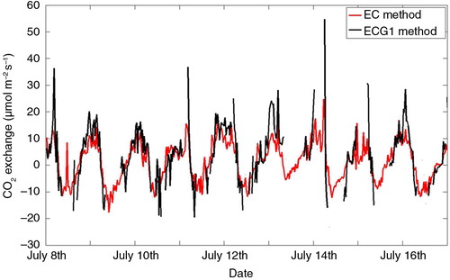
Good agreement was found between CO₂ fluxes calculated by ECG method and CO₂ fluxes from EC measurements (Fig. 2). The ECG method captures seasonal and diel variations well, although it tends to overestimate peak respiration values. Fluxes from the two methods are significantly correlated with p<0.001 and a Pearson correlation coefficient of 0.80.

Fig. 2 Comparison of net CO₂ exchange measured by EC at 33 m and net CO₂ exchange calculated from gradients between 31.7 and 58.8 m by combined EC and gradient method (ECG) in July 2010. For the ECG method, only values with good accuracy, i.e., total errors <20 µmol m⁻² h⁻¹, are shown (see text for details).

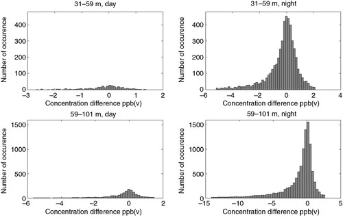
Errors in CH₄ concentration gradient measurements were the major contributors to errors in calculated CH₄ fluxes. Observed CH₄ gradients were small most of the time, especially during daytime, where the concentration difference between levels was usually <1 ppb (Fig. 3a) due to strong turbulence. At night, turbulence is often weak and concentrations at different levels are distinctly different (Fig. 3b). Frequency distributions of CH₄ concentration gradients during day and night after selection of data sets are shown in Fig. 4.

Fig. 3 Example of (a) daytime and (b) nighttime CH₄ concentration measurements. Each level (31.7, 58.8 and 100.6 m) was measured for 5 min=300 s starting at level 1.

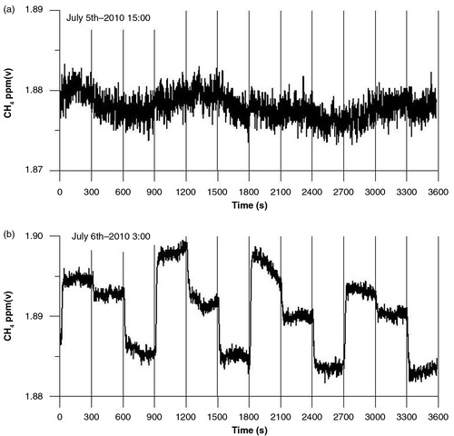
Fig. 4 Occurrence of CH₄ concentration differences for different height intervals and for day (global radiation >50 Wm⁻²) and night (global radiation <50 Wm⁻²). Data between the 2nd and 98th percentiles are shown.

3.2. Atmospheric CH₄ concentrations and net CH₄ exchange

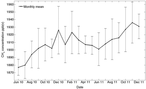
The atmospheric concentration of CH₄ measured at 100.6 m varied over the season from 1875 to 1930 ppb, with a distinct minimum during the summer months. A trend of increasing concentrations was observed over the measurement period (Fig. 5).

Fig. 5 CH₄ concentration measured at 100.6 m height from June 2010 to December 2011. Error bars are given as plus/minus SD of monthly mean concentrations.

Taking the entire measurement period and all wind directions into account, the Norunda site is a net source of CH₄ according to both flux calculation methods. Mean emissions at the site were 2.57, 4.57, 1.48 and 2.99 µmol m² h⁻¹ for BR1, BR2, ECG1 and ECG2, respectively.

For the study period, the main wind directions at the site were S to SW (Fig. 6). Emissions from these directions were lower in comparison with peak emissions at NW to NE wind directions (Fig. 7). Monthly mean values of CH₄ exchange from S to SW (June 2010–December 2011) are listed in Table 1.

Fig. 6 Windrose for Norunda site at 33 m height above ground for the entire measurement period.

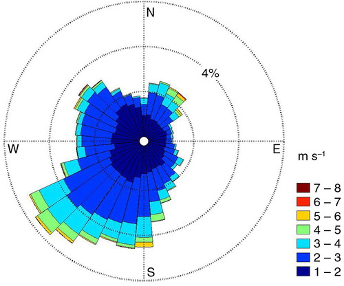
Fig. 7 Average CH₄ exchange at the tower for wind directions binned in 30 degree intervals.

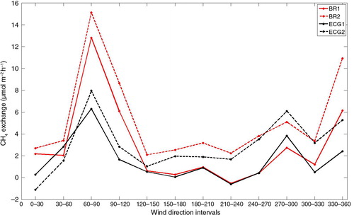
Table 1. Monthly mean values of CH₄ exchange for main wind directions, 180°–240°, derived using the modified Bowen ratio (BR) method and the combined eddy covariance and gradient method (ECG) for gradients between 31.7 and 58.5 m and between 31.7 m and 100.6 m

	BR1 CH4 exchange (µmol m^−2 h^−1)	BR2 CH4 exchange (µmol m^−2 h^−1)	ECG1 CH4 exchange (µmol m^−2 h^−1)	ECG2 CH4 exchange (µmol m^−2 h^−1)	Chambers CH4 exchange (µmol m^−2 h^−1)
Jun 2010	7.5	8.7	4.0	8.0	–
Jul 2010	1.95	5.6	1.2*	3.8	−11.7
Aug 2010	−1.7	2.1	−2.7	2.4	−9.8
Sep2010	3.9	5.9	2.5	5.9	−9.0
Oct 2010	2.7	5.3	4.1	5.5	–
Nov2010	0.7*	2.8	−0.7*	3.0	–
Dec2010	−1.6	1.7*	−1.9	1.1*	–
Mar 2011	0.3*	3.5	1.0	2.2	–
Apr 2011	3.1	3.9	5.9	6.6	–
May 2011	−0.3*	1.7	−1.4*	1.2	–
Jun 2011	0.2*	5.2	1.1*	3.9	–
Jul 2011	−1.2*	1.3*	−1.2*	0.1*	–
Aug 2011	−4.0	1.1*	−3.7	1.8	–
Sept2011	−2.7	1.1*	−1.6*	0.4*	–
Oct 2011	0.3*	0.9*	0.1*	0.2*	–
Nov 2011	−1.1	−0.1*	−1.4	−1.4	–
Dec 2011	−1.4	0.4*	−3.1	−0.4*	–

*Not significantly different from zero.

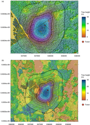
The 90% level of the footprints for gradients measured between 31.7 and 58.8 m were within 500 m from the tower (Fig. 8a) while the footprints for gradients measured between 31.7 and 100.6 m reached almost 1 km from the tower. A large part of the clear-cut was within the 70% level of the footprint (Fig. 8b), i.e., emissions from the clear-cut were measured with high probability at the higher level.

Fig. 8 Half-hourly footprint estimates cumulated for the entire measurement period for (a) gradients between 31.7 and 58.5 m and (b) between 31.7 and 100.6 m. Contour lines are plotted for each 10% of the cumulated footprint. The tower location is depicted as a red dot. The background maps are tree height from LiDAR measurements, for illustration. Coordinates (x and y axes) are in UTM.

3.3. Seasonal and diel variations and drivers of CH₄ exchange

For the entire measurement period, the CH₄ exchange ranged from a minimum uptake of −4.0 µmol m⁻² h⁻¹ in August 2011 by BR1 to maximum emissions of 8.7 µmol m⁻² h⁻¹ in June 2010 by BR2. According to BR1 and ECG1, there was a net average CH₄ uptake for the main wind direction (180°–240°) for the months August 2010, December 2010, May 2011, July to September 2011 and November to December 2011 (Table 1). BR2 and ECG2 showed reduced emissions for most of these months except for summer 2011 (Table 1). Weekly average values of CH₄ exchange from BR1 and ECG1 originating from the main wind direction, as well as environmental conditions at the site for the entire measuring period, are shown in Fig. 9.

Fig. 9 Weekly mean values of CH₄ exchange, water table depths, air temperature and soil temperature and also the weekly amount of precipitation.

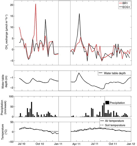
Water table depth and CO₂ exchange significantly contributed in explaining variations in the CH₄ exchange according to multiple linear regression analyses (Table 2). Negative fluxes had a tendency to coincide with lower ground water table, and the largest positive fluxes in 2011 coincided with high ground water table (Fig. 9). CO₂ exchange showed higher correlation with CH₄ exchange for BR1 and BR2, which might be a consequence of the BR method using CO₂ exchange for calculation of CH₄ exchange. Combinations of air temperature, soil temperature, soil moisture, water table depth, CO₂ exchange and gross primary production (GPP) could only explain 3–23% of variations in CH₄ exchange (Table 2).

Table 2. Coefficients calculated by multiple linear regression analyses of daily mean values of CH₄ exchange derived at two levels and for two different methods (the modified Bowen ratio (BR) method and combined eddy covariance and gradient method (ECG)); and the explanatory variables air temperature, soil temperature, soil moisture, water table depth, CO₂ exchange and GPP. The analysis was made on standardised data to adjust for the disparity in variable sample sizes. The adjusted R ² value displays how much of the variance in CH₄ exchange can be explained

	ECG1		ECG2		BR1		BR2
	Jun–Sep, N=97, R ^2=0.03	Total, N=200, R ^2=0.07	Jun–Sep, N=126, R ^2=0.05	Total, N=281, R ^2=0.07	Jun–Sep, N=114 R ^2=0.1	Total, N=265, R ^2=0.18	Jun–Sep, N=136 R ^2=0.14	Total, N=300, R ^2=0.23
Air temperature	−0.09	0.035	−0.0005	0.05	−0.06	−0.05	0.04	−0.1
Soil temperature	−0.1	−0.004	−0.03	0.09	−0.07	−0.09	−0.01	−0.36*
Soil moisture	0.05	0.1	0.09	0.14	0.009	0.01	0.03	0.09
Water table depth	0.24*	0.30*	0.23*	0.25*	0.39*	0.32*	0.27*	0.19*
CO2 flux	−0.1	0.0006	0.23*	0.23*	0.1	0.36*	0.30*	0.64*
GPP	−0.07	−0.06	−0.03	0.03	0.04	0.1	0.12	0.37*

*The variable significantly contributes to the variance in CH₄.

Diel variations in CH₄ exchange were apparent when data were binned hourly (Fig. 10). CH₄ emissions reached a maximum just before dawn (approximately 05:00) local time and then decreased during the day to minima in late afternoon 15:00–18:00 local time. The diel pattern was evident in fluxes derived by both BR and ECG methods but was most pronounced for BR1. The amplitudes of the diel variation in CH₄ exchange curves were in the order of5–8 µmol m⁻² h⁻¹. We looked closer at diel variations of BR1 since it has a more homogeneous footprint than BR2 and ECG2 and because more daytime values of CH₄ exchange passed the quality criteria (cf. section 2.4) than for ECG1. Correlations between hourly binned CH₄ exchange for BR1 and hourly binned soil temperature, air temperature, GPP and vapour pressure deficit (VPD) are listed in Table 3. Significant correlations at p<0.05 were found for all variables depending on season. Correlations were strongest for air temperature and GPP. Soil CH₄ exchange measured by chambers did not show a consistent diel pattern (Fig. 11).

Fig. 10 Diel pattern of CH₄ exchange binned hourly for the entire measurement period.

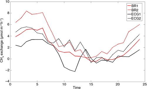
Fig. 11 Diel patterns of soil CH₄ exchange measured by individual soil chambers, 7 July–31 September 2010.

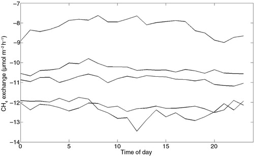
Table 3. Pearson correlations between hourly binned CH₄ exchange for BR1 and hourly binned air temperature, soil temperature, GPP and VPD

	Air temperature	Soil temperature	GPP	VPD
Mar–Apr	−0.50*	0.54*	0.85**	−0.68**
May–Jun	−0.54*	−0.15	0.49*	−0.46*
Jul–Aug	−0.77**	0.19	0.80**	−0.58*
Sep–Oct	−0.79**	−0.19	0.68**	−0.68**
Nov–Dec	−0.26	−0.12	0.24	−0.17
Total	0.26	0.56*	0.88**	−0.52*

*Significant at p<0.05, *significant at p<0.001.

3.4. Chamber measurements

In contrast to gradient measurements, the soil chamber measurements from July to September 2010 indicated that the soil was a sink of CH₄ of around −10 µmol m⁻² h⁻¹ (Table 1). These rates are similar in magnitude to previously reported forest soil uptake rates (e.g., Smith et al., 2000).

4. Discussion

4.1. Net CH₄ exchange

Previous comparisons of chamber measurements and MM measurements of CH₄ exchange within forests have shown good agreement of fluxes (Querino et al., 2011; Wang et al., 2013; Yu et al., 2013). However, in this study, gradient measurements above the canopy indicate that the forest is a net source of CH₄, which is in strong contrast to local small spatial-scale chamber measurements showing net CH₄ uptake by the ground surface. A possible reason for the discrepancy is that the gradient measurements are influenced by a large forest area (up to 1 km radius) with higher variability in net CH₄ soil fluxes than represented by the chambers, which were situated in the vicinity of the tower (within 100 m). Simpson et al. (1997) also report net CH₄ emissions measured by gradients above canopy and net CH₄ uptake measured below the canopy in the vicinity of their tower. They ascribed the difference to emissions of CH₄ from wet patches emitting CH₄, located within the footprint of the tower-based above-canopy measurements. Another reason for the discrepancy could be possible emissions from the canopy or from the trunks of the trees (see Section 4.3).

4.2. Impact of wind direction and footprint

At Norunda, the clear-cut located within the footprint at 500 m to the west of the tower (Fig. 8b) is a well-characterised source area (Sundqvist et al., 2014). Higher than average emissions were observed for these westerly wind directions. Additional possible sources of CH₄ at Norunda are more clear-cuts, lakes and wetlands at 1–2 km distance from the tower. These areas are outside the flux footprint of the gradient-based flux measurements. However, at this site, and for the higher level especially, the requirement of horizontally homogeneous fluxes for the application of Horst's method (Horst, 1999) is not fulfilled. Keeping in mind that footprints for concentration measurements are typically 2–3 times larger than those of flux measurements, the CH₄ sources at larger distances might still contribute to some extent to the measurements at higher levels. Peak emissions in E and NW directions (Fig. 8b) could be explained by distant sources if seen by both upper air intakes, but are probably explained by sources from wet soils within the footprint.

Emissions from the dominant wind direction are low in comparison to other wind directions and during some months a net uptake of −1 to −3 µmol m⁻² h⁻¹ is measured using BR1 and ECG1 (Table 1). However, CH₄ uptake measured at the soil surface by chambers was many times larger, about −10 µmol m⁻² h⁻¹. Patches of wetter soils and small ponds can be found in the main wind direction and it is possible that emissions from these wet areas switch the site from being a sink of CH₄ to being a source of CH₄ as shown by BR2 and ECG2 and for some months by BR1 and ECG1 (Table 1). Temporal shifts of soils from net sinks to net sources in wet periods were found in several studies (e.g., Hudgens and Yavitt, 1997; Moosavi and Crill, 1997; Sakabe et al., 2012). Observations further indicate that large emissions from small source areas can shift a site from a sink to a source (Fiedler et al., 2005; Sakabe et al., 2012).

4.3. Impact of vegetation

Quantitative linkages of below canopy processes and above canopy measurements tend to be difficult to analyse. In addition, since all air intakes for the gradient measurements were positioned above the canopy, it is not possible to distinguish soil emissions from within canopy exchanges. Most MM measurement studies have not detected substantial aerobic CH₄ emissions from vegetation (Bowling et al., 2009; Querino et al., 2011; Ueyama et al., 2012; Wang et al., 2013), but Mikkelsen et al. (2011) found indications for CH₄ emissions from a beech forest stand during a period of low wind conditions. However, microbial production of CH₄ in the wet heartwood of trees has been known for at least 40 yr (Zeikus and Ward, 1974). Furthermore, trees can transport and release CH₄ from soil water (Gauci et al., 2010; Terazawa et al., 2007).

Laboratory studies have shown that aerobic CH₄ emissions from vegetation could be triggered by UV radiation and heating (Vigano et al., 2008), but emissions in the absence of UV have also been measured, although at much lower rates (Bruhn et al., 2009). If canopy emissions caused by high UV radiation were a major contribution to CH₄ exchange at the Norunda site, we would expect the emissions to peak during daytime and not at night as observed in this study (Fig. 10).

4.4. Seasonal variations and drivers of CH₄ exchange

Reduced CH₄ emissions in summer, as shown in Fig. 9, can be due to a decrease in water table depth and soil moisture, which counteracts methanogenic production and favours methanotrophic oxidation, by decreasing the depth of the methanogenic zone in the soil and facilitating diffusion of atmospheric CH₄ and oxygen to methanotrophs. In 2011, the water table depth had continuously dropped on average since the snowmelt in April, which may have resulted in shifting formerly wet areas from CH₄ sources to CH₄ sinks. In addition, the positive effect of reductions in water table depth and soil moisture on methanotrophic uptake might have outweighed an increase in CH₄ emission due to increases in soil temperatures which could have been expected otherwise. Peak emissions coincide with a high water table as observed following precipitation and snowmelt (see for example, June 2010, September 2010 and April 2011 in Fig. 9). Multiple linear regression analyses revealed a significant relationship between CH₄ exchange and water table depth for both gradient methods (Table 2).

The reduction of atmospheric CH₄ concentrations during summer (Fig. 5) cannot be interpreted as a result of an increased soil uptake, since seasonal patterns in CH₄ concentrations are expected to mainly depend on an increased destruction of atmospheric CH₄ by hydroxyl radicals, and the production of hydroxyl radicals in the atmosphere is larger in summer (Khalil and Rasmussen 1983). At high southern latitude sites, land-based CH₄ sources and sinks are very small and the seasonal CH₄ cycle is dominated by variability in hydroxyl radical production. The seasonal amplitude is about 30 ppb (Dlugokencky et al., 1994), which is about the same size as the amplitude of the CH₄ concentration cycle at Norunda. In a forested landscape with the absence of larger wetlands and antropogenic sources, it is likely that seasonal variations in atmospheric CH₄ concentrations mainly follow the cycle of hydroxyl radicals. The observed trend of increasing CH₄ concentrations over the study time period could simply be a result of local year-to-year variability. Several years of data would be needed to validate this trend.

4.5. Diel pattern

Diel variations in CH₄ exchange at Norunda seem independent of the season, except for November–December where no diel pattern could be found. It should be kept in mind that about 90% of the daytime data were removed due to too small gradients. To rule out that the observed diel pattern was an artefact caused by unequal sample size, we also estimated diurnal curves by randomly sampling equal amounts of data points from each bin for BR1. This procedure clearly revealed a reproducible and consistent diel pattern. Emissions were highest during the night or early morning hours and lowest in the afternoon (Fig. 10). Querino et al. (2011) observed nighttime maxima in CH₄ flux associated to venting below canopy storage depletion. However, at Norunda this explanation does not hold as CH₄ gradients change gradually over many hours. Pattey et al. (2006) measured net CH₄ emissions at a boreal forest site using a gradient method and assigned higher daytime temperatures to be the cause of higher emissions. Since at Norunda, net CH₄ emissions dominate above the canopy, we might expect similar daytime enhancements due to temperature dependence of methanogens, but during most of the time CH₄ exchange was negatively correlated with temperature (Table 3). This suggests that temperature-independent processes affect the net flux.

Periods with lower than average CH₄ emissions at Norunda might be due to methanotrophs dominating the net flux. Diel trends with maximum CH₄ uptake around noon were found at sites where consumption dominates the CH₄ exchange (Smeets et al., 2009; Sakabe et al., 2012; Wang et al., 2013). Wang et al. (2013) explained the increased daytime uptake with increased turbulence during the day that facilitated the transport of atmospheric CH₄ to the methanotrophs in the soil, while Sakabe et al. (2012) found a dependency of the diel amplitude of CH₄ exchange on air temperature. We know from chamber measurements (Sundqvist et al., 2014) that CH₄ uptake in well-aerated forest soil could benefit from both increased turbulence and increases in soil temperatures. However, our chamber measurements do not show a consistent diel pattern (Fig. 11).

Distant source areas could possibly explain the diel pattern, since their contributions would be larger at night than during daytime due to reduced turbulence at night. Variability in fluxes is also higher during nighttime than during daytime. A possible explanation for this could be the smaller daytime footprint that includes mainly homogeneous upland forest. During nighttime, however, the sources can vary much more as the footprints are larger and the surroundings of the main forest show higher heterogeneity further away including more wet areas.

Plant uptake could also contribute to the observed diel pattern of CH₄ exchange. A net uptake of CH₄ by shoots and leaves of spruce, pine, rowan and birch has been measured at Norunda (Sundqvist et al., 2012). The uptake increased with increasing photosynthetically active radiation. On a larger scale, just as with CH₄ emissions, we have no means to distinguish uptake by soil from uptake by vegetation. The diel curve of CH₄ exchange correlates with GPP (Table 3), and because diel variation of GPP is largely controlled by incoming radiation, it seems possible that uptake by vegetation impacts the diel CH₄ pattern.

5. Summary and conclusions

We used a modified BR method and a combined ECG method to quantify the methane (CH₄) exchange between canopy and the overlaying atmosphere at the Norunda forest site in central Sweden. Good agreement between CO₂ fluxes calculated by the ECG method and CO₂ fluxes measured by the EC method indicate that the ECG method should also provide reliable results for CH₄ fluxes. However, subtle gradients, especially during daytime, coupled to cumulative error due to ambient variability and instrumentation limitations considerably reduced the number of measurements during data processing. Fluxes calculated by the BR method and the ECG method are of similar order of magnitudes. According to both BR and ECG methods, the site is a net source of CH₄ of 1.48–4.57 µmol m⁻² h⁻¹. This finding is in contrast to chamber measurements in the study area which indicate that the soil is a net sink of CH₄ of −10 µmol m⁻² h⁻¹. The only well-characterised source area within the footprint of the tower is a clear-cut area, which is located within the 70% footprint level for ECG and BR when gradients between 31.7 and 100.6 m are considered. Peak emissions from smaller wet patches within the forest might turn the site from a sink to a source despite an uptake in well-aerated soil. All air intakes of the gradient measurements were positioned above the canopy; therefore, it is not possible to discriminate between soil CH₄ exchange and any canopy CH₄ exchange. The CH₄ exchange follows a clear diel pattern, with higher net emissions at night and lower net emissions in the afternoon. The decrease in net emissions during afternoon hours might be a result of an uptake by the canopy since the diel pattern of CH₄ exchange correlates with both GPP and VPD which indicates that there might be a coupling between the CH₄ exchange and photosynthesis. A diel pattern could also be explained by contributions from more distant source areas, which would have a larger impact at night due to longer horizontal transport vectors during low turbulence conditions.

6. Acknowledgements

This work was supported by Formas and the Linnaeus Centre LUCCI (www.lucci.lu.se/index.html) funded by the Swedish Research Council. This was also supported by INGOS FP7 Project (AL and MM). Airborne LiDAR for the Norunda site was acquired with support from the British Natural Environment Research Council (NERC/ARSF/FSF grant EU10-01 and NERC/GEF grant 933). We thank Anders Båth for field assistance.

References

- Baldocchi D. , Falge E. , Gu L. H. , Olson R. , Hollinger D. , co-authors . FLUXNET: a new tool to study the temporal and spatial variability of ecosystem-scale carbon dioxide, water vapour, and energy flux densities. BAMS. 2001; 82: 2415–2434.
- Born M. , Doerr H. , Levin I . Methane consumption in aerated soils of the temperate zone. Tellus B. 1990; 42: 2–8.
- Bowling D. R. , Miller J. B. , Rhodes M. E. , Burns S. P. , Monson R. K. , etal. Soil, plant, and transport influences on methane in a subalpine forest under high ultraviolet irradiance. Biogeosciences. 2009; 6: 1311–1324.
- Bradford M. A. , Ineson P. , Wookey P. A. , Lappin-Scott H. M . Soil CH4 oxidation: response to forest clearcutting and thinning. Soil Biol. Biochem. 2000; 32: 1035–1038.
- Bruhn D. , Mikkelsen T. N. , Obro J. , Willats W. G. T. , Ambus P . Effects of temperature, ultraviolet radiation and pectin methyl esterase on aerobic methane release from plant material. Plant Biol. 2009; 11: 43–48.
- Castro M. S. , Melillo J. M. , Steudler P. A. , Chapman J. W . Soil-moisture as a predictor of methane uptake by temperate forest soils. Can. J. Forest Res. 1994; 24: 1805–1810.
- Crill P. M. , Martikainen P. J. , Nykanen H. , Silvola J . Temperature and N-fertilization effects on methane oxidation in a drained peatland soil. Soil Biol. Biochem. 1994; 26: 1331–1339.
- Denmead O. T . Approaches to measuring fluxes of methane and nitrous oxide between landscapes and the atmosphere. Plant Soil. 2008; 309: 5–24.
- Dlugokencky E. J. , Steel L. P. , Lang P. M. , Masarie K. A . The growth-rate and distribution of atmospheric methane. J. Geophys. Res-Atmos. 1994; 99: 17021–17043.
- Dunfield P. , Knowles R. , Dumont R. , Moore T. R . Methane production and consumption in temperate and sub-arctic peat soils – response to temperature and pH. Soil Biol. Biochem. 1993; 25: 321–326.
- Ehhalt D. H . Atmospheric cycle of methane. Tellus. 1974; 26: 58–70.
- Fiedler S. , Holl B. S. , Jungkunst H. F . Methane budget of a Black Forest spruce ecosystem considering soil pattern. Biogeochemistry. 2005; 76: 1–20.
- Foken T . Micrometeorology. 2008; Berlin Heidelberg: Springer-Verlag. 179–222.
- Gauci V. , Gowing D. J. G. , Hornibrook E. R. C. , Davis J. M. , Dise N. B . Woody stem methane emission in mature wetland alder trees. Atmos. Environ. 2010; 44: 2157–2160.
- Grunwald D. , Fender A. C. , Erasmi S. , Jungkunst H. F . Towards improved bottom-up inventories of methane from the European land surface. Atmos. Environ. 2012; 51: 203–211.
- Guckland A. , Flessa H. , Prenzel J . Controls of temporal and spatial variability of methane uptake in soils of a temperate deciduous forest with different abundance of European beech (Fagus sylvatica L.). Soil Biol. Biochem. 2009; 41: 1659–1667.
- Harriss R. C. , Sebacher D. I. , Day F. P . Methane flux in the great dismal swamp. Nature. 1982; 297: 673–674.
- Högstrøm U . Non-dimensional wind and temperature profiles in the atmospheric surface-layer- a re-evaluation. Boundary-Layer Meteorol. 1988; 42: 55–78.
- Horst T. W . The footprint for estimation of atmosphere-surface exchange fluxes by profile techniques. Boundary-Layer Meteorol. 1999; 90: 171–188.
- Hudgens D. E. , Yavitt J. B . Land-use effects on soil methane and carbon dioxide fluxes in forests near Ithaca, New York. Ecoscience. 1997; 4: 214–222.
- Kammann C. , Hepp S. , Lenhart K. , Mulller C . Stimulation of methane consumption by endogenous CH4 production in aerobic grassland soil. Soil Biol. Biochem. 2009; 41: 622–629.
- Keller M. , Reiners W. A . Soil atmosphere exchange of nitrous-oxide, nitric-oxide, and methane under secondary succession of pasture to forest c lowlands of Costa-Rica. Global Biogeochem. Cy. 1994; 8: 399–409.
- Khalil M. A. K. , Rasmussen R. A . Sources, siks and seasonal cycles of atmospheric methane. J Geophys. Res. 1983; 88: 5131–5144.
- Kljun N. , Calanca P. , Rotach M. W. , Schmid H. P . A simple parameterisation for flux footprint predictions. Boundary-Layer Meteorol. 2004; 112: 503–523.
- Kljun N. , Rotach M. W. , Schmid H. P . A three-dimensional backward Lagrangian footprint model for a wide range of boundary-layer stratifications. Boundary-Layer Meteorol. 2002; 103: 205–226.
- Koschorreck M. , Conrad R . Oxidation of atmospheric methane in soil – measurements in the field, in soils cores and in soil samples. Global Biogeochem. Cy. 1993; 7: 109–121.
- Lessard R. , Rochette P. , Topp E. , Pattey E. , Desjardins R. L. , co-authors . Methane and carbon-dioxide fluxes from poorly drained adjacent cultivated and forest sites. Can J Soil Sci. 1994; 74: 139–146.
- Lundin L. C. , Halldin S. , Lindroth A. , Cienciala E. , Grelle A. , co-authors . Continuous long-term measurements of soil-plant-atmosphere variables at a forest site. Agr. Forest Meteorol. 1999; 98–9: 53–73.
- Mikkelsen T. N. , Bruhn D. , Ambus P. , Larsen K. S. , Ibrom A. , co-authors . Is methane released from the forest canopy?. iForest. 2011; 4: 200–204.
- Mölder M. , Grelle A. , Lindroth A. , Halldin S . Flux-profile relationships over a boreal forest – roughness sublayer corrections. Agr. Forest Meteorol. 1999; 98–9: 645–658.
- Moncrieff J. B. , Massheder J. M. , de Bruin H. , Elbers J. , Friborg T. , co-authors . A system to measure surface fluxes of momentum, sensible heat, water vapor and carbon dioxide. J. Hydrol. 1997; 188–189: 589–611.
- Moosavi S. C. , Crill P. M . Controls on CH4 and CO2 emissions along two moisture gradients in the Canadian boreal zone. J. Geophys. Res-Atmos. 1997; 102: 29261–29277.
- Nicolini G. , Castaldi S. , Fratini G. , Valentini R . A literature overview of micrometeorological CH4 and N2O flux measurements in terrestrial ecosystems. Atmos Environ. 2013; 81: 311–319.
- Pattey E. , Strachan I. B. , Desjardins R. L. , Edwards G. C. , Dow D. , co-authors . Application of a tunable diode laser to the measurement of CH4 and N2O fluxes from field to landscape scale using several micrometeorological techniques. Agr. Forest Meteorol. 2006; 136: 222–236.
- Physick W. L. , Garratt J. R . Incorporation of a high-roughness lower boundary into a mesoscale model for studies of dry deposition over complex terrain. Boundary-Layer Meteorol. 1995; 74: 55–71.
- Querino C. A. S. , Smeets C. , Vigano I. , Holzinger R. , Moura V. , co-authors . Methane flux, vertical gradient and mixing ratio measurements in a tropical forest. Atmos. Chem. Phys. 2011; 11: 7943–7953.
- Rotach M. W. , Gryning S. E. , Tassone C . A two-dimensional stochastic Lagrangian dispersion model for daytime conditions. Quart. J. Roy. Meteorol. Soc. 1996; 122: 367–389.
- Rotach M. W . Simulation of urban-scale dispersion using a Lagrangian stochastic dispersion model. Bound Layer Meteor. 2001; 99: 379–410.
- Sakabe A. , Hamotani K. , Kosugi Y. , Ueyama M. , Takahashi K. , co-authors . Measurement of methane flux over an evergreen coniferous forest canopy using a relaxed eddy accumulation system with tuneable diode laser spectroscopy detection. Theor. Appl. Climatol. 2012; 109: 39–49.
- Shoemaker J. K. , Keenan F. T. , Hollinger D. Y. , Richardson A. D . Forest ecosystem changes from annual methane source to sink depending on late summer water balance. Geophys. Res. Lett. 2014; 41: 637–679.
- Simpson I. J. , Edwards G. C. , Thurtell G. W. , den Hartog G. , Neumann H. H. , co-authors . Micrometeorological measurements of methane and nitrous oxide exchange above a boreal aspen forest. J. Geophys. Res-Atmos. 1997; 102: 29331–29341.
- Smeets C. , Holzinger R. , Vigano I. , Goldstein A. H. , Rockmann T . Eddy covariance methane measurements at a Ponderosa pine plantation in California. Atmos. Chem. Phys. 2009; 9: 8365–8375.
- Smith K. A. , Dobbie K. E. , Ball B. C. , Bakken L. R. , Sitaula B. K. , co-authors . Oxidation of atmospheric methane in Northern European soils, comparison with other ecosystems, and uncertainties in the global terrestrial sink. Glob. Change Biol. 2000; 6: 791–803.
- Sundqvist E. , Crill P. , Mölder M. , Vestin P. , Lindroth A . Atmospheric methane removal by boreal plants. Geophys. Res. Lett. 2012; 39
- Sundqvist E. , Vestin P. , Crill P. , Persson T. , Lindroth A . Short-term effects of thinning, clear-cutting and stump harvesting on methane exchange in a boreal forest. Biogeosciences. 2014; 11: 6095–6105.
- Terazawa K. , Ishizuka S. , Sakatac T. , Yamada K. , Takahashi M . Methane emissions from stems of Fraxinus mandshurica var. japonica trees in a floodplain forest. Soil Biol. Biochem. 2007; 39: 2689–2692.
- Ueyama M. , Hamotani K. , Nishimura W. , Takahashi Y. , Saigusa N. , co-authors . Continuous measurement of methane flux over a larch forest using a relaxed eddy accumulation method. Theor. Appl. Climatol. 2012; 109: 461–472.
- Vigano I. , Van Weelden H. , Holzinger R. , Keppler F. , McLeod A. , co-authors . Effect of UV radiation and temperature on the emission of methane from plant biomass and structural components. Biogeosciences. 2008; 5: 937–947.
- Von Fischer J. C. , Hedin L. O . Separating methane production and consumption with a field-based isotope pool dilution technique. Global Biogeochem. Cy. 2002; 16: 8/1–8/13.
- Wang F. L. , Bettany J. R . Methane emission from a usually well-drained prairie soil after snowmelt and precipitation. Can J Soil Sci. 1995; 75: 239–241.
- Wang J. M. , Murphy J. G. , Geddes J. A. , Winsborough C. L. , Basiliko N. , co-authors . Methane fluxes measured by eddy covariance and static chamber techniques at a temperate forest in central Ontario, Canada. Biogeosciences. 2013; 10: 4371–4382.
- Whalen S. C. , Reeburgh W. S . Consumption of atmospheric methane by tundra soils. Nature. 1990; 346: 160–162.
- Whalen S. C. , Reeburgh W. S . Moisture and temperature sensitivity of CH4 oxidation in boreal soils. Soil Biol. Biochem. 1996; 28: 1271–1281.
- Yu K. W. , Faulkner S. P. , Baldwin M. J . Effect of hydrological conditions on nitrous oxide, methane, and carbon dioxide dynamics in a bottomland hardwood forest and its implication for soil carbon sequestration: Glob. Change Biol. 2008; 14: 798–812.
- Yu L. F. , Wang H. , Wang G. S. , Song W. M. , Huang Y. , co-authors . A comparison of methane emission measurements using eddy covariance and manual and automated chamber-based techniques in Tibetan Plateau alpine wetland. Environ. Pollut. 2013; 181: 81–90.
- Yvon-Durocher G. , Allen P. A. , Bastviken B. , Conrad R. , Gudasz C. , co-authors . Methane fluxes show consistent temperature dependence across microbial to ecosystem scales. Nature. 2014; 507: 488–491.
- Zeikus J. G. , Ward J. C . Methane formation in living trees-microbial origin. Science. 1974; 184: 1181–1183.