Consistency of tropospheric ozone observations made by different platforms and techniques in the global databases

Abstract

A large quantity of tropospheric ozone observations are conducted all over the world using different platforms and techniques for different purposes and goals. These observations are commonly used to derive seasonal cycles, interannual variations and long-term trends of ozone in the troposphere. In addition, they are used for comparison with three-dimensional chemistry-transport models to evaluate their performance and hence to test our current understanding of the tropospheric ozone variability. It is still challenging to provide robust tropospheric ozone trends throughout the world because of the great variability of ozone, its complex photochemical reactions, the rarity of long-term records, the diversity of measurement techniques and platforms, and the issues with data quality. In this work, we evaluated, with emphasis on the lower troposphere, the consistency of tropospheric ozone observations made by means of multiple platforms, including surface sites, sondes and regular aircraft, that are publicly available in the global databases, but excluding space-borne platforms. Concomitant observations were examined on an hourly basis (except for ±3 hours for sonde versus aircraft) for pairs of locations at less than 100-km distance. Generally, we found good agreement between sonde and surface observations. We also found that there was no need to apply any correction factor to ozonesonde observations except for Brewer–Mast sondes at Hohenpeissenberg. Because of a larger distance between the site pairs, the correlations found between the aircraft and surface measurements were poorer than those between sonde and surface measurements. However, a relatively simple wind segregation improved the agreement between the aircraft versus surface measurements. We found also that due to diurnal cycles, the sonde launching at a fixed local time led to positive or negative biases against the surface observations, suggesting that great attention should be paid to local time and diurnal variations when using ozonesonde in the analysis of seasonal cycles, long-term trends and interannual variations of lower tropospheric ozone. The comparison of surface data at Mt. Happo to regular aircraft data over Tokyo/Narita showed a relatively reasonable agreement, ensuring regionally representative ozone data sets in this region for trend analysis.

• tropospheric ozone
• MOZAIC
• IAGOS
• WDCGG
• WOUDC

This paper is part of a Special Issue on MOZAIC/IAGOS in Tellus B celebrating 20 years of an ongoing air chemistry-climate research measurement from airbus commercial aircraft operated by an international consortium of countries. More papers from this issue can be found at http://www.tellusb.net

1. Introduction

Tropospheric ozone (O₃) is one of the most important constituents of the Earth's atmosphere. It greatly contributes to global warming by absorbing infrared radiation and causes detrimental effects to human health, forest trees and agricultural crops. The latest estimate for the global mean radiative forcing of tropospheric O₃ is 0.356±0.58 W m⁻² as an ensemble mean of 17 chemistry-climate models (Stevenson et al., 2013). This value is the third among greenhouse gases next to methane (CH₄). Along with black carbon (BC), tropospheric O₃ is recognised as one of short-lived climate pollutants (SLCPs), in contrast to long-lived greenhouse gases such as CO₂ (UNEP/WMO, 2011). Recently, the role of reducing SLCPs in climate change mitigation in the near future has been highlighted (Shindell et al., 2012). Thus, controlling the emissions of both ozone precursors (NOx, VOC, etc.) and BC will benefit simultaneous mitigation of air pollution and climate change, in particular in developing countries. Air quality standards [also called ‘criteria’ in some countries or ‘guidelines’ by the World Health Organization (WHO)] are set for ground-level O₃, generally because of the adverse effects on human health. One of the major health impacts is the increase of premature deaths due to the increase of O₃. The WHO evaluated the increase in daily mortality rate with 8-hour average O₃ to be 1–2% for 50 nmol mol⁻¹ (hereafter referred to as ppb) and 3–5% for 80 ppb (WHO, 2006). The detrimental impacts of O₃ on terrestrial ecosystems are also well known. Using indexes to estimate the impact of O₃ on vegetation, such as Accumulated Ozone Over Threshold (AOT40) (Fuhrer et al., 1997), the global economic loss due to ambient level O₃ in 2000 for major agricultural crops such as wheat, rice, corn and soybean, has been revealed to be quite substantial (Van Dingenen et al., 2009).

There is growing evidence that tropospheric O₃ has increased in the Northern Hemisphere during the past century (Parrish et al., 2012). Historical records of tropospheric O₃ in Europe have shown an apparent increase in the baseline O₃ levels during the 20th century (Voltz and Kley, 1988; Staehelin et al., 1994). More recent studies have reported that the boundary-layer O₃ has been rising in recent decades at mid-latitudes in both the Northern Hemisphere (Lee et al., 1998; Jaffe et al., 2003; Naja and Akimoto, 2004; Simmonds et al., 2004; Oltmans et al., 2006; Zbinden et al., 2006; Derwent et al., 2007; Tanimoto et al., 2009; Parrish et al., 2012) and the Southern Hemisphere (Lelieveld et al., 2004), likely as a result of increasing NOx emissions. According to those studies, the overall growth rates range from 0.5 to 0.8 ppb yr⁻¹. A large increase of approximately 1.0 ppb yr⁻¹ was observed at Mt. Happo until 2007, where the observations largely reflected the free tropospheric air (Tanimoto, 2009). These observations of tropospheric O₃ were analysed using chemistry-transport models (CTMs). However, the CTM simulations have not yet quantitatively explained the observed increase of tropospheric O₃ in East Asia (Tanimoto et al., 2009) and in the entire Northern Hemisphere (Parrish et al., 2014). The changes in NOx have imposed significant perturbations on the levels, variability and trends of tropospheric O₃ on local, regional and hemispheric scales. Tropospheric O₃ pollution is widely spread across the entire Northern Hemisphere due to long-range transport on an intercontinental scale (Wild and Akimoto, 2001), and may affect local air quality, contributing to the violation of national ambient air quality. The increasing changes in tropospheric O₃ in the Northern Hemisphere have substantial impacts on the climate and ecosystem of the Earth.

Measurements by ozonesondes had been often used to analyse the spatial and temporal variations of O₃ in the troposphere during the past decades (Oltmans et al., 1998, 2006, 2013; Logan, 1994; Logan et al., 1999; Naja and Akimoto, 2004). In particular until the 1990s, the primary source of information on long-term changes of tropospheric O₃ was the ozonesonde records. Although some surface stations started measurements in the 1970s, the number of monitoring sites increased in the early 1990s. By the early 2000s, the data from continuous measurements at ground-based stations in remote and rural areas, operated as a contribution to international programmes (e.g. WMO/GAW, EANET), have been used for the analysis of the long-term trends of surface O₃. Beginning in the mid-1990s, measurements of tropospheric and lower stratospheric O₃ by regular aircraft have been successfully made.

The data sets of tropospheric O₃ observations have been used to analyse seasonal cycles, interannual variations and long-term trends, and to evaluate and/or validate the performance and capability of global/regional three-dimensional CTMs. It is often the case that different data sets are used for the trend analysis for different regions and different periods of time. For model validation, the representativeness of the sites and observation errors are concerned, partly because the tropospheric O₃ observations are made using different platforms and techniques for different purposes and goals. On the other hand, the databases that offer scientists the use of the data of tropospheric O₃ observations have had considerable improvement during the recent years. The integration of the data of tropospheric O₃ obtained using different platforms/techniques has great potential to better understand the evolution of tropospheric O₃ and to improve the models.

In spite of this potential, there have been few efforts to test the consistency of the data of tropospheric O₃ measurements. Logan et al. (2012) tested the consistency of observations made by ozonesondes, regular aircraft and from alpine surface sites over Europe. Saunois et al. (2012) examined the uncertainty caused by the sampling frequency of ozonesondes for the analysis of long-term trends. Tilmes et al. (2012) evaluated the regional representativeness of tropospheric O₃ in the northern mid-latitudes and high latitudes by comparing observations using ozonesondes and regular aircraft. Zbinden et al. (2013) evaluated the ozonesonde observations with reference to aircraft observations for the altitude of 2–8 km in time coincidence and found that the differences were −7%, −2% and +0.9% [Measurements of Ozone and water vapour by in-service Aircraft (MOZAIC) minus World Ozone and Ultraviolet Radiation Data Centre (WOUDC)] over eastern United States, Germany and Japan, respectively. Although focused on stratospheric observations, international efforts have been made to evaluate the data quality of O₃ observations, and the uncertainties of measurements by ozonesondes, ground-based remote sensing instruments and satellite sensors have been summarised (SPARC, 1998; Hassler et al., 2014). To make climatological data sets for the stratosphere, Toohey et al. (2013) pointed out the importance of non-uniform temporal sampling for producing monthly means by satellites. Staufer et al. (2013) evaluated the consistency of O₃ data obtained by ozonesondes and the MOZAIC aircraft in the upper troposphere/lower stratosphere by using the trajectory matching technique, and found considerable differences of up to 25% in ozonesondes at the 28 ozonesonde sites against MOZAIC measurements in the mid-1990s, followed by smaller differences of around 5–10% in later years (Staufer et al., 2014). All of these results warrant further examination of the consistency of O₃ observations by different platforms and techniques, in order to achieve robust data sets to analyse climatology and long-term trends when compared to models.

In most cases of trend analysis and model validation, monthly means are used. The specific aims of this work are to evaluate the comparability of tropospheric O₃ data available in different databases and to assess its impacts when using monthly means in the analysis and interpretation of seasonal cycles, interannual variations and long-term trends, and model validation, with strong emphasis on lower tropospheric O₃.

2. Data and methods

We used long-term data sets of tropospheric O₃ observations available in the global databases as summarised in Table 1. The source of data used for the present analysis is three global databases that are publicly available. The first database is operated as part of the Global Atmosphere Watch (GAW) programme of the World Meteorological Organization, namely WOUDC (www.woudc.org) supported by Environment Canada. The second is the World Data Centre for Greenhouse Gases (WDCGG, www.ds.data.jma.go.jp/gmd/wdcgg/), supported by the Japan Meteorological Agency. The third is the In service Aircraft for Global Observing System (IAGOS, www.iagos.fr/) database including the historical MOZAIC (www.iagos.fr/mozaic) data and the Civil Aircraft for the Regular Investigation of the atmosphere Based on an Instrument Container (CARIBIC, www.caribic-atmospheric.com) project data.

Table 1. Summary of tropospheric ozone measurements available in databases

Platform	Sonde	Surface	Regular aircraft
Technique	Wet electro-chemical	UV absorption	UV absorption
Location	Remote – rural	Remote – rural	International airports
Vertical coverage	Troposphere/stratosphere	Ground surface only	Troposphere/lower stratosphere
Local time	Fixed local time	Continuous	Variable
Sampling frequency	Every 1–2 weeks	Continuous	Variable
Database	WMO/WOUDC	WMO/WDCGG	MOZAIC-IAGOS

These data sets are different in their characteristics: (1) the measurement techniques, hence associated uncertainties (accuracy, precision and error) are different from each other. Measurements by sonde are based on a wet electro-chemical method, while surface and aircraft measurements are based on photometric absorption in the ultraviolet wavelength region; (2) the site locations are different. Generally, sonde and surface measurements are made in rural and remote areas, while regular aircraft measurements rely on international airports, which are often in the city or its suburb; (3) the vertical coverages are different between surface and other measurements. Ozonesonde measurements cover an area from the ground surface up to approximately 35 km, and the profiles by aircraft measurements cover up to 12 km, the typical cruising altitude of regular international aircraft in the lower stratosphere (in case of domestic connections, the maximum altitude is reduced due to the short-time duration of flights); (4) the local time (LT) and sampling frequency can also differ. Sondes are launched at a fixed LT with a typical frequency of every week. Surface measurements are basically made on a continuous basis, except for occasional instrument malfunction or maintenance. In contrast, LT and measurement frequencies are variable and sometimes even unpredictable for aircraft measurements depending on flight schedules of the equipped aircraft, since interruption in the routine flight services can happen. The measurement methods used in the databases are as follows.

• Sonde: for ozonesondes, three sensor types are reported in the WOUDC database: the Carbon Iodine (CI; or KC: KI solution and Carbon electrode), the Brewer–Mast (BM) and the Electro-chemical Concentration Cell (ECC). The ECC is the most widely used sensor, and the BM type is used only at Hohenpeissenberg in Germany, while the CI type was used in Tateno/Tsukuba in Japan until November 2009. The O₃ parameter in this data set is labelled ‘O₃PartialPressure’ to calculate the O₃ mixing ratios at each altitude level defined as ‘GPHeight’. For each profile a correction factor (CF) is suggested by the WOUDC to scale the profile so that the columns computed agree with the total O₃ column (for which the stratospheric fraction is dominant) measurements using co-located ground-based and/or overpassing satellite instruments (Morris et al., 2013). For tropospheric O₃, the uncertainty of sonde measurements is estimated to be 3–5% and 5–10% by ECC type and other types, respectively (Smit et al., 2007; Hassler et al., 2014). The effective vertical resolution of ozonesondes is about 100–150 m (Hassler et al., 2014).

• Surface: O₃ measurements in the WDCGG database are compiled from past and current monitoring carried out in international, regional and individual research projects. Many of the sites are operated by national meteorological agencies as part of the GAW programme of the World Meteorological Organization (WMO, 2007), and the data are quality controlled. Typically ‘O₃’ data determined by ultraviolet absorption technique are used.

  In addition to the WDCGG data sets, data at Mt. Happo [36.69°N, 137.80°E, 1850 m asl. (above sea level)] are being collected, since the long-term O₃ trend at Mt. Happo had been previously examined as the data were largely affected by the free tropospheric air masses, showing an intriguingly increasing trend during the last decades (Tanimoto et al., 2009; Parrish et al., 2012). The site is operated by the Ministry of the Environment of Japan as part of the Acid Deposition Monitoring Network in East Asia (EANET) programme (Network Center for EANET, 2007).

  In both the EANET and GAW programmes, the mixing ratios of O₃ are determined using photometric instruments based on absorption of light at 253.7 nm emitted by a low-pressure mercury lamp. The Standard Reference Photometer (SRP) #2 at the National Institute of Standards and Technology (NIST) is used as the primary standard, which the O₃ mixing ratios are scaled to. The data are scrutinised in the post-analysis, including Quality Assurance/Quality Control (QA/QC) activities and are then made available to the public. The uncertainty of O₃ measurements is estimated to be ±2 ppb. Consistency of standards and traceability for ground-level O₃ observations in East Asia including the GAW and EANET programmes have been directly assessed (Tanimoto et al., 2007).

• Aircraft: the MOZAIC programme has collected a huge amount of O₃ observation data (and H₂O, CO, NOy along with meteorological parameters) between August 1994 and November 2014 by using instruments onboard up to five commercial aircraft (Marenco et al., 1998; Thouret et al., 2006) throughout the troposphere and lower stratosphere. IAGOS has taken over since 2011 with five aircraft already in operation (www.iagos.org; Thouret and Petzold, 2014; Petzold et al., 2015). Measurement technique for O₃ remains the same. The O₃ mixing ratios are measured using the dual-beam UV-absorption principle (Model 49-103 from Thermo Environmental Instruments, Franklin, MA, USA, modified according to aeronautical constraints), with an uncertainty estimated at ±2 ppb and a 4 seconds time response, that is, <50 m vertical resolution (Thouret et al., 1998). Measurement quality control procedures have remained unchanged since the beginning of the programme to ensure that long-term series are free of instrumental artefacts. Instruments are laboratory calibrated before and after a flight period of about 6–12 months. For MOZAIC-IAGOS, ‘ozone_vmr’ (or ‘O₃’) is used along with ‘baro altitude’. To characterise the vertical distribution over the troposphere, we use the ascents and descents of the flights at high resolution (4 seconds, 28–40 m vertically).

We set up rigorous criteria for this study in order to examine the data quality of the measurements in the individual databases. In more detail, we examined (1) the uncertainties arising from the differences in measurement techniques, site locations, and sampling time and frequency, and (2) the consequences on the seasonal cycles, interannual variations and long-term trends of tropospheric O₃. Comparisons by selecting only concomitant observations were made to see to what extent this data processing could improve the consistency of data from different databases. A time matching (or temporal coincidence) of 1 hour was assessed for the comparisons between the sonde WOUDC and the surface WDCGG data, and between the aircraft MOZAIC-IAGOS and surface WDCGG data, because the surface WDCGG instruments are operated continuously. The time matching for the comparison between sonde WOUDC and aircraft MOZAIC-IAGOS observations was within ±3 hours. To be more precise, we only used the data when ascent or descent between the surface and 9 km had been made within an hour, and when the mean time of the ascent or descent was within ±3 hours of the launching time of ozonesondes (e.g. from 11:30 to 17:30 LT for MOZAIC-IAGOS over Tokyo/Narita to 14:30 LT for ozonesondes in Tateno/Tsukuba). To avoid any stratospheric influence, we only used data of ‘pure’ tropospheric O₃ as determined by Zbinden et al. (2013). This horizontal distance between the two sites compared had to be less than approximately 100 km. This threshold is far well within the distance with which we can expect good correlative behaviour for the lower troposphere (Liu et al., 2009). The vertical layers for the comparisons of the sonde WOUDC and the aircraft MOZAIC-IAGOS data to the surface WDCGG observations was fixed to approximately 200 m (typically 5–20 data points for both sonde and aircraft, depending on the aircraft speed), referenced to the altitude of the surface sites (e.g. the 950–1150 m data for Hohenpeissenberg site at 986 m, the 2300–2500 m data for Izana site at 2367 m). This is because of a substantial vertical gradient below 1 km above the ground surface (Zbinden et al., 2013). The vertical profiles at many MOZAIC-IAGOS sites (e.g. Frankfurt, Munich, Tokyo/Narita, Osaka/Kansai) show lower O₃ levels near the ground surface with a magnitude up to 20 ppb below 1-km altitude. The time was LT unless otherwise noted.

3. Results and discussion

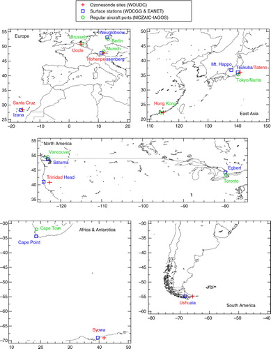
Figure 1 is a map showing the sites where we found pairs of O₃ measurements that met the criteria mentioned above. For the sonde versus surface comparisons, six sites in Germany, Japan, Spain, Argentina and USA were found. For the aircraft versus surface comparisons, six sites in Germany, Japan, Canada and South Africa were identified. For the comparisons between sondes and aircraft, eight sites were found, but of these, four sites in South Africa, Malaysia, USA and Kenya had only a few time-coincident observations. Hence, we used only four sites in Belgium, Germany, Japan and Hong Kong for the rigorous comparisons. Many site pairs are located in the Northern Hemisphere, in particular, in Europe, North America and East Asia, where long-term O₃ trends have been extensively analysed by using the data of O₃ measurements by sondes, regular aircraft and at surface sites. At two locations, Hohenpeissenberg (and Munich) and Tateno/Tsukuba (and Tokyo/Narita), the three types of observations (i.e. sondes, regular aircraft and surface sites) were subject to in-depth comparisons.

Fig. 1 Global distribution of the sites of sonde, surface and regular aircraft observations examined in this work.

3.1. Comparison of sonde with surface observations

Table 2 lists the sites of the sonde and surface observations used in the comparisons. Among these comparisons, the sonde and surface observations were made at the same locations by the same organisations at Hohenpeissenberg (HPB), Tateno/Tsukuba (Tateno is a former name of this location and the name Tsukuba is currently used. Hence for simplicity, hereafter we refer to Tsukuba, TKB), Syowa (SYO) and Ushuaia (USH). There are nearly 1600 data pairs available for comparison at HPB with BM-type sondes since 1995. In TKB and SYO, nearly 90% of the data have been obtained using the CI-type sensor until 2009, and a marginal 10% using the ECC type since 2010 and onwards. The O₃ data at other stations are based on the ECC-type sonde, with data pairs of a few hundreds until now. On Tenerife Islands, the ground site of the Izana Atmospheric Research Centre (IZO) is located at 2367 m asl., while sondes are launched in Santa Cruz at 36 m asl. These sites are within a distance of 27 km.

Table 2. Characteristics of the sites measuring tropospheric ozone, relevant for the sonde and surface comparisons

Country	Sonde WOUDC	STN	Surface WDCGG	ID	Distance (km)	Period	Number of matched hourly data
Germany	Hohenpeissenberg (976 m)	99	Hohenpeissenberg (985 m)	HPB	~0	1995–2007	BM: 1598
Japan	Tateno/Tsukuba (31 m)	14	Tsukuba (25 m)	TKB	~0	1988–2012	1115 (CI: 989, ECC: 126)
Japan	Syowa (22 m)	101	Syowa (16 m)	SYO	~0	1999–2012	720 (CI: 631, ECC: 89)
Spain	Santa Cruz (36 m)	401	Izana (2367 m)	IZO	~27	2008–2012	ECC: 291
Argentina	Ushuaia (17 m)	339	Ushuaia (18 m)	USH	~0	1996–2003	ECC: 126
USA	Trinidad Head (107 m)	445	Trinidad Head (120 m)	THD	~28	2004–2006	ECC: 85

Ozonesonde types are BM: Brewer–Mast; CI: Carbon Iodine (or KC: KI solution and Carbon electrode); ECC: Electro-chemical Concentration Cell.

In this comparison, we first examined how application of the CF to ozonesonde observations affects the ozonesonde data, and thereby the agreement to the surface observations. Table 3 summarises the slopes, intercepts and correlation coefficients with and without applying CF for the scatter plots of tropospheric O₃ mixing ratios measured by sondes versus those measured at surface sites. CF is available for four sites, namely HPB, TKB, SYO and USH. CF is dedicated to judge the quality of the O₃ profile measured by ozonesondes up to the burst altitude and may be applied to correct the data. Profiles with CF outside the prescribed limits are usually rejected. For ECC- and CI-sondes, the limits are often set in the range 0.80–1.20, and for BM-sondes used at HPB it is 0.90–1.50 (SPARC, 1998). As a result, when applying CF to the ozonesonde records, only one site (HPB) showed an improvement in the slope (8%), while the correlation coefficient did not significantly change. For the other sites (TKB, SYO and USH), better slopes and correlation coefficients were found without CF, thus the application of CF did not improve the agreement. This is in accordance with the fact that the profiles by BM-sondes used at HPB are generally scaled to total ozone column measurements by about +5–15% (Smit and ASOPOS Panel, 2013). Hence, we used the CF-applied data at HPB only, and not at other three sites in the following discussion.

Table 3. Effects of correction factor (CF) on the agreement between ozonesonde measurements and surface observations of tropospheric ozone

Sonde	Slope		Intercept (ppb)		Correlation coefficient
WOUDC	w/o CF	w CF	w/o CF	w CF	w/o CF	w CF
Hohenpeissenberg	0.81 (0.01)	0.89 (0.01)	0.2 (0.3)	−1.2 (0.4)	0.92	0.90
Tateno/Tsukuba	1.00 (0.01)	1.02 (0.02)	−2.2 (0.6)	−5.2 (0.8)	0.89	0.82
Syowa	1.09 (0.03)	1.19 (0.03)	−6.8 (0.7)	−0.2 (0.9)	0.74	0.66
Santa Cruz	1.23 (0.04)	–	−8.0 (2.1)	–	0.78	–
Ushuaia	1.01 (0.05)	1.56 (0.12)	0.9 (1.2)	−10.3 (2.8)	0.83	0.51
Trinidad Head	1.03 (0.06)	–	−2.7 (1.9)	–	0.82	–

In parentheses are the associated 95% confidence levels. The data in bold are selected for Fig. 2. w/o CF: without correction factor; w CF: with correction factor.

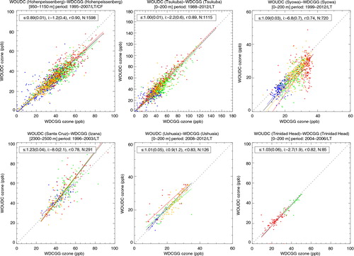
Figure 2 shows the scatter plots of tropospheric O₃ mixing ratios measured by sonde versus those measured at surface sites. We found, generally, good correlative behaviours between sonde and surface observations for the six pairs of sites, with regression lines being close to the 1:1 corresponding lines. In HPB, the correlation is generally strong, whereas the overall slope is 0.89. This indicates that even when CF is applied, measurements by BM-sondes are still underestimated by approximately 10%, suggesting that other factors must be taken into consideration. This issue will be discussed later. In TKB, the range of O₃ mixing ratios is up to 150 ppb and the correlation is reasonably high, with a slope of 1.0. At SYO, the correlation is poorer than that in TKB, although the ozonesondes in TKB and SYO are operated by the same agency. The plots are more scattered in the range 30–40 ppb for the summer (JJA) period. As a result, we see significant negative offsets and highly biased slopes regardless of season for sonde against surface observations. Although there are less data available for comparisons at IZO, USH and THD (Trinidad Head), the correlation coefficients for these sites are approximately 0.8 with a slope of approximately 1.0 at USH and THD and 1.2 at IZO.

Fig. 2 Scatter plots of tropospheric ozone mixing ratios measured by sondes versus those measured at surface sites. The data and regression lines for winter (DJF), spring (MAM), summer (JJA) and fall (SON) are illustrated with blue, green, red, and orange symbols, respectively. The regression line for all the data is illustrated in black, and its slope (s), intercept (i), correlation coefficient (r) and data number (N) are denoted with the associated 95% confidence level. The correction factor (CF) is applied to the ozonesonde data at Hohenpeissenberg, but not at the other five sites.

Similar to Fig. 2, the scatter plots of tropospheric O₃ mixing ratios measured by sonde versus those measured at surface sites, with different sensor types only in TKB and SYO, are shown in Fig. 3. The effects of CF are also shown for both sensor types. Since ozonesonde measurements by the Japan Meteorological Agency have been made using CI until recently (2009 for TKB and 2010 for SYO), nearly 90% of the data pairs at these two stations are dominated by CI measurements. Hence, the overall features for the measurements using CI sensor are basically the same as those seen in Fig. 2. In contrast, the measurements by ECC show higher correlations, with coefficients of 0.98 for TKB and 0.96 for SYO. The slope and intercept are greatly improved at SYO, although the number of data pairs is only 89. Although it was reported that CF has little impact on the mean tropospheric profile obtained by CI-sondes in Japan (Morris et al., 2013), we found significant effects of CF on the agreement of CI-sondes to the surface data. Although with the limited number of data, ECC-sondes did not show any significant difference by the application of CF. It is known that the scaling effect for ECC-sondes is only a few percent, because normalisation of ECC-sondes gives an average CF near 1.0 (SPARC, 1998). Our results confirmed the robustness of the O₃ observations by ECC-sondes.

Fig. 3 Same as Fig. 2 but for different sensor types for sondes [left, Carbon Iodine (CI); right, Electro-chemical Concentration Cell (ECC)] in Tsukuba (top panel) and Syowa (bottom panel). The plots show the data both with CF (blue) and without CF (red).

3.2. Comparison of aircraft with surface observations

Table 4 lists the sites of aircraft and surface observations used in the comparison. In contrast to the comparison between sonde and surface measurements, aircraft and surface observations are not made at the same stations. Generally, the distances between the site pairs are in a range of 40–80 km. Lower tropospheric O₃ measurements by aircraft rely on ascent from and descent to the airports. There are more than 1000 data pairs available for comparison at HPB and TKB since the mid-1990s. In HPB, the ground station is located at 985 m asl., while the Munich International Airport is located at 453 m asl. Other sites are located at similar heights (within ±200 m).

Table 4. Characteristics of the sites where tropospheric ozone is measured, relevant for the aircraft and surface comparisons

Country	Aircraft MOZAIC-IAGOS	IATA	Surface WDCGG	ID	Distance (km)	Period	Number of matched hourly data
Germany	Munich (453 m)	MUC	Hohenpeissenberg (985 m)	HPB	84	1996–2006	2059
Japan	Tokyo/Narita (43 m)	NRT	Tsukuba (25 m)	TKB	40	1995–2012	1113
Canada	Toronto (173 m)	YYZ	Egbert (253 m)	EGB	62	1994–2003	271
Canada	Vancouver (4 m)	YVR	Saturna (178 m)	SAT	46	1998–2003	135
South Africa	Cape Town (46 m)	CPT	Cape Point (230 m)	CPT	44	1998–2009	57
Germany	Berlin (37 m)	TXL	Neuglobsow (65 m)	NGL	70	1994–2004	37

Figure 4 shows the scatter plots of tropospheric O₃ mixing ratios measured by aircraft versus those measured at surface sites. For all the comparisons, there are relatively good correlative behaviours between the aircraft and surface observations. However, the comparisons are associated with lower correlation coefficients (r) than those between sonde and surface observations, suggesting that the agreement was poorer. The major reason can be attributed to larger distances between the sites for the aircraft versus surface measurements than between the sonde versus surface measurements, as also suggested by the spatial correlation analysis with ozonesondes at 1 km altitude (Liu et al., 2009). At HPB, there is generally a high correlation with negligible intercept, with the overall slope being nearly 0.97. There seems to be a large scattering below 30 ppb in wintertime. This is likely because the boundary layers in wintertime are shallow above the ground surface, resulting in comparisons of different air masses, for example, boundary-layer air over HPB and free tropospheric air over Munich. In TKB, the correlation to Narita (NRT) looks rather poor. The correlation coefficient is worse than that in HPB and that of sonde versus surface observations in TKB. The disagreement is remarkable, in particular in the summer (JJA) season, with higher or lower biases. The difference of locations is one influencing factor for this large disagreement. Also this disagreement may be due to the interplaying roles of meteorology from local to regional scales, including land-sea breeze in the Tokyo Bay area (Chang et al., 1989) and the Asian monsoon that brings maritime air masses from the Pacific Ocean in this season. In Egbert (EGB), Saturna (SAT), Cape Point (CPT) and Neuglobsow (NGL), the correlation coefficients are in the range of 0.64–0.80. The low correlation suggests that the values of the MOZAIC measurements are lower than those of the surface measurements in EGB. In this analysis, only a limited number of data pairs were available in SAT, CPT and NGL. More data pairs are needed to draw robust conclusions for these comparisons.

Fig. 4 Scatter plots of tropospheric ozone mixing ratios measured by regular aircraft versus those measured at surface sites. Plus symbols indicate the data pairs after wind selection.

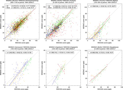
For the HPB versus MUC and for the TKB versus NRT comparisons, we examined how the agreement could be improved when the data were segregated by local wind (i.e. wind direction and speed). HPB is located southwest of MUC with a distance of ~84 km, and TKB is located northwest of NRT with a distance of ~40 km. We segregated the O₃ data by using the MOZAIC wind data at MUC and NRT. We selected data pairs only when the local wind direction suggested that the air masses at MUC and NRT came from the locations of HPB and TKB, respectively. The width of wind direction was set to ±15° and the threshold of wind speed was set to 2 m s⁻¹. This segregation resulted in the number of data pairs to be reduced to 4% at MUC and 13% at NRT. This exercise successfully excluded the majority of outlier data and the large scattering seen in the original plots, resulting in an obvious improvement in the degree of correlation. The improvement is also apparent from the improved correlation coefficients at both sites (from 0.77 to 0.84 for HPB versus MUC and from 0.57 to 0.82 for TKB versus NRT). These results have the important implication that relatively simple wind selection can help identify regionally representative data and enhance statistical robustness in the analysis. The correlation coefficients of about 0.8 for these site pairs are in reasonable accordance with those found by Liu et al. (2009). It is interesting to note that a good correlation was found between the near surface O₃ at HPB and the O₃ over MUC, which is thought to be free from surface deposition and more affected by free tropospheric air masses.

3.3. Comparison of aircraft with sonde observations

As shown in Fig. 1, there are eight sites that met the criteria for the comparisons of aircraft and sonde observations. After considering the time-matching criteria, that is, that both measurements were made within ±3 hours, only four site pairs in Brussels-Uccle, Munich-Hohenpeissenberg, Tokyo/Narita-Tsukuba and Hong Kong have remained with substantial data numbers. Other site pairs include those in South Africa [Johannesburg International Airport (JNB), 1694 m asl., and Irene, 1524 m asl., distance of 26 km], Malaysia [Kuala Lumpur International Airport (KUL) at 21 m asl. and Sepang at 17 m asl., distance of 2 km], USA [Boston Logan International Airport (BOS), 6 m asl. and Narragansett, 21 m asl., distance of 101 km], and Kenya [Jomo Kenyatta International Airport (NBO), 1625 m asl. and Nairobi, 1795 m asl., distance of 16 km]. However, for these sites the number of data meeting the criteria is less than 5, mainly due to a short overlapping period of time (1–7 yrs). Hence, we did not include these comparisons in this work. These sites could be included in the future work, if enough amounts of data have been submitted to the data centres in the future. The sites listed in Table 5 were used for the comparison of tropospheric O₃ between regular aircraft observations and sonde observations. For these four pairs, the distances between the sites are in a range from 20 to 84 km. For BRU and MUC, there are more than 300 matched pairs, while NRT has nearly 100 pairs, and Hong Kong (HKG) has only 20 pairs.

Table 5. Characteristics of the sites where tropospheric ozone is measured, relevant for the aircraft and sonde comparisons

Country	Aircraft MOZAIC-IAGOS	IATA	Sonde WOUDC	STN	Distance (km)	Period	Number of matched hourly data^a
Belgium	Brussels (56 m)	BRU	Uccle (100 m)	53	20	1997–2009	ECC: 566
Germany	Munich (453 m)	MUC	Hohenpeissenberg (976 m)	99	84	1998–2006	BM: 327
Japan	Tokyo/Narita (43 m)	NRT	Tateno/Tsukuba (31 m)	14	40	1996–2012	98 (CI: 97, ECC: 1)
Hong Kong	Hong Kong (9 m)	HKG	Hong Kong (66 m)	344	28	2000–2010	20

^aWithin ±3 hours.

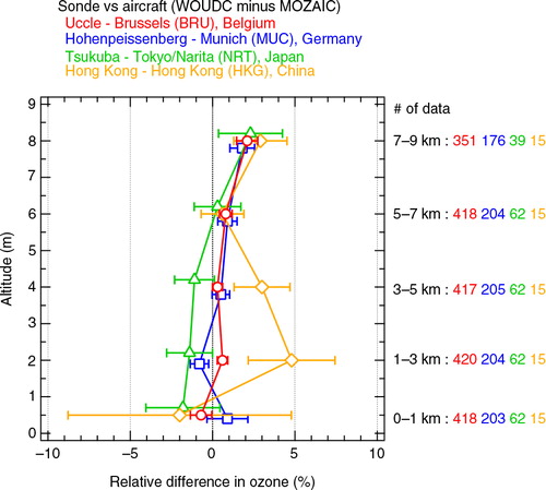
Figure 5 illustrates the relative differences in O₃ (sonde minus aircraft observations relative to the average of the two observations) at 5 altitude levels between 0 and 9 km. The number of site pair matching is less for the 7–9 km altitude level than those lower, since some data were omitted due to stratospheric influence at this altitude level. Eventually, the comparisons of BRU versus Uccle, and MUC versus HPB at the individual levels have approximately 400 and 200 matched pairs, respectively. The comparisons of the sondes to MOZAIC-IAGOS indicate a reasonable agreement within approximately ±2% at all altitude levels up to 9 km for the ECC-sondes at Uccle, the BM-sondes at HPB, and the CI-sondes at TKB, while the CI-sondes tend to have somewhat negative biases. Staufer et al. (2014) made a similar analysis using the trajectory matching technique with a focus on the middle troposphere and the upper troposphere/lower stratosphere, over 28 sites. The agreement over Uccle and Tsukuba in recent years has been within ±5%, showing a general agreement with our work. The comparison over HKG at the lower tropospheric levels showed large positive biases and uncertainties, which can be attributed to overestimates by sondes. This difference can be due to the artefact by other oxidants like sulphur dioxides co-existing in the same air masses. The very limited amount of data is also a factor to produce large confidence limits. We note a better agreement for the sites associated with more data pairs. More data would lead to a better quality of trends obtained from the sonde and aircraft measurements.

Fig. 5 Medians of the relative differences in tropospheric ozone mixing ratios for five altitude levels measured by sondes and regular aircraft. Error bars denote the 95% confidence level.

3.4. Consistency of seasonality and long-term trends

An important question is whether the seasonal cycles, interannual variations and long-term trends of O₃ can be captured consistently from ‘in-situ’ instruments at any tropospheric level, and more precisely, within the boundary layer where we can compare the three types of O₃ measurements. Next, we will focus on two sites, Hohenpeissenberg/Munich and Tsukuba/Narita, where we can compare all of the sonde, surface and aircraft observations, and discuss their consistency.

3.4.1. Time series

Figure 6 shows the time series plots of tropospheric O₃ mixing ratios measured by sondes, regular aircraft and surface observations for five altitude levels at HPB/MUC and TKB/NRT, from 1995 to 2012. Although three data sets are available for the 0–1 km level at HPB, we note that the surface measurements and sonde launching at HPB were made at 985 m, while aircraft profiles were obtained over 453 m over MUC. As can be expected from the previous discussion, the surface data show higher O₃ mixing ratios than the others, in particular the sondes. The large peak in summer 2003, as seen in the HPB surface and sonde observations up to 5 km, is a result of enhanced O₃ records due to a heat wave in Europe (Tressol et al., 2008, synthesising MOZAIC data over Paris, Munich and mainly Frankfurt). Here, we note that the MOZAIC time series over Munich suffers from a lack of data between 4 July and 14 August, and thus MOZAIC data over Munich do not display the O₃ enhanced mixing ratios because of the heat wave in summer 2003, highlighting random sampling issue. There is a good general agreement between the sonde and aircraft observations in the free troposphere. This confirms the need for CF to obtain accurate O₃ mixing ratios by BM-sondes. In spite of the good agreement of sondes with aircraft data in the free troposphere, the sondes are still underestimated below 1 km, suggesting that CF cannot sufficiently correct the O₃ data by BM-sondes near the ground surface. Despite the excellent agreement in concomitant data between the MOZAIC data over MUC and the surface data at HPB, the monthly MOZAIC data are substantially lower than the surface data at HPB for 0–1 km. This is due to the steep gradient in O₃ below 1 km, and the MOZAIC data are the average of 453–1000 m, while the surface data are of 985–1000 m.

Fig. 6 Time series of tropospheric ozone mixing ratios measured by sondes, regular aircraft and at surface stations for five altitude levels in the troposphere at Hohenpeissenberg (left) and Tsukuba (right).

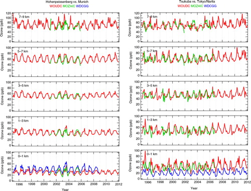
In TKB, the MOZAIC data are available for the period from 1995 to 2006, suggesting a reasonable agreement with sonde measurements in general. However, the agreement below 3 km seems to be poorer than that above 3 km, in particular during the summer season. The large variability indicates the effects of limited sampling frequency for statistical averages, coupled with local pollution below 3 km over Tsukuba.

3.4.2. Seasonal cycles

Figure 7 indicates the seasonal cycles of tropospheric O₃ at five altitude layers at HPB and TKB measured by sonde, aircraft and surface observations. The data plotted are simple monthly means with no data selection by time matching, as usually adopted for data analysis or model evaluation. At HPB, the three different types of observations show good overlaps with each other, suggesting that the seasonal cycles are well documented either by sonde, surface or aircraft observations. The seasonal cycles show a broad summer maximum, which is a characteristic of the photochemical O₃ production in the troposphere. Over the course of 1 yr the sonde data are lower than the surface data by 5–15 ppb, associated with a maximum in the summer season.

Fig. 7 Seasonal cycles of tropospheric ozone mixing ratios measured by sondes, regular aircraft and at surface stations at different altitudes at Hohenpeissenberg (left) and Tsukuba (right). The sonde-minus-surface differences in O₃ are expressed by pink dotted lines for the right axis. The dashed blue line in Tsukuba shows the seasonal cycle of the surface observations based only on the 14:00–15:00 LT data.

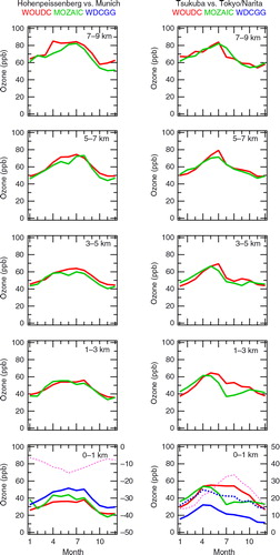
In TKB, we see a good general agreement between sonde and aircraft observations from 3 to 9 km, showing a maximum in springtime. However, a substantial difference can be seen between sonde and aircraft observations below 3 km down to the ground surface. This discrepancy is most pronounced below 1 km, especially with regard to surface observations, which show much lower O₃ values than the other methods. The aircraft observations by MOZAIC show a spring peak with a summer minimum, which is a typical seasonal cycle in this Asian Pacific rim region. The surface observations also show a spring peak, though the levels are much lower than those obtained by the MOZAIC observations. In contrast, sonde measurements show a broad summertime maximum. To understand this discrepancy, it should be noted that ozonesondes are regularly launched at a fixed LT (14:30 LT in the case of TKB). This is in sharp contrast to surface observations, for which the monthly means are calculated from continuous data. The MOZAIC aircraft observations are made at various LTs, depending on the fleet schedules. These are typically during 07:00–14:00 LT for Japan including Tokyo/Narita, Osaka/Kansai and Nagoya. Therefore, we extracted the data at 14:00–15:00 LT from the surface observations in TKB, calculated monthly means and compared them to the other observation methods. The O₃ levels obtained by surface observations increased by 15 ppb over the course of a year, resulting in improved agreement with the other observation methods. The differences among the three observation means are negligible in the cold season (October–April), whereas still substantial in the warm season (May–September).

To further examine the effects of sampling time on the agreement among the different means of observation, the diurnal cycles of the surface and sonde data collected at HPB and TKB are shown in Fig. 8. In HPB, we found from the surface observations that diurnal cycles were negligible in winter but substantial in other seasons, in particular spring and summer with an amplitude of approximately 10 ppb, due to photochemical O₃ build-up during the daytime and an O₃ loss by surface deposition during the night. Although the sonde data are in agreement within the uncertainty with the surface data at the time when the sondes were launched, the sonde data are substantially lower than the daily means calculated from the 24-hour surface measurements. This negative bias happens because the sondes are launched at HPB in the early morning when the diurnal cycle of O₃ takes a minimum or is greatly lower than the daily means in spring and summer. This can explain why the sonde data are lower than the surface data in the spring and summer seasons.

Fig. 8 Mean diurnal cycles of tropospheric ozone mixing ratios at the surface level in Hohenpeissenberg and Tsukuba, as measured using surface stations and sondes. Vertical error bars denote one standard deviation and horizontal error bars for Hohenpeissenberg denote the range of time for the sonde launching. Dashed lines are daily means calculated from the surface data.

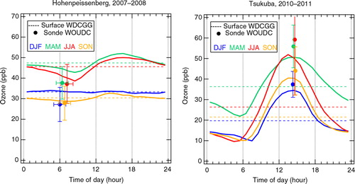
In TKB, we found from the surface observations that the diurnal cycles were substantially large throughout the year. Since TKB is located in a sub-urban area (within 50 km) in the greater Tokyo metropolitan area, photochemical O₃ build-up during the daytime and an O₃ loss by titration during the night are common phenomena. The amplitude is 25 ppb in winter but is enhanced to 40 ppb in summer. Here again, although the sonde data are in agreement within the uncertainty with the surface data at the time when the sondes were launched, the sondes data are substantially higher than the daily means calculated from the surface measurements. This positive bias happens because the sondes are launched at TKB in the early afternoon, when the diurnal cycle of O₃ takes a maximum or much higher values than the daily means. Owing to the greater amplitude in summer, the discrepancy between sonde and surface measurements is also greater in summer. In the analysis of seasonal cycles and long-term trends, caution must be paid to two factors to avoid possible positive or negative biases: the LT of the sonde launching and the amplitude of diurnal cycles around the sonde sites.

In Fig. 9, we compared the monthly mean O₃ data calculated from all the available data to that calculated from only concomitant data (as we described above), for the ozonesonde and MOZAIC aircraft observations against surface observations. At HPB, the correlation between the MOZAIC aircraft and the surface measurements shows a reasonable agreement, while the correlation between the ozonesonde and the surface measurements indicates a systematically underestimated bias by 10–20% for the ozonesondes. The correlation is stronger for the concomitant data than for all the data, as can be seen from considerably improved correlation coefficients (r) from 0.83 to 0.90 for the MOZAIC versus surface data and from 0.89 to 0.94 for the ozonesonde versus surface data. The slopes are also improved for both sonde and aircraft observations. The slope improved from 0.80 to 0.88 for the sonde. The comparison between surface and sonde measurements suggests that out of 20% underestimation of sondes, 8% is from diurnal cycles, and remaining 12% is from other sources including local conditions for the sondes [e.g. the height of sonde launching is lower (1 m above the ground surface) than that of the sampling inlet at the top of the tower (18 m at HPB) for the surface observations].

Fig. 9 Scatter plots of monthly mean ozone measured by sondes, regular aircraft and surface stations, made of all (left) and concomitant (right) hourly data at Hohenpeissenberg (top panel) and Tsukuba (bottom panel).

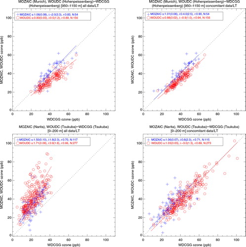
In the scatter plots of the monthly means made of all the data in TKB (Fig. 9), it can be seen that both the MOZAIC and the sonde data show 50–70% higher O₃ levels than the surface data. When using concomitant data, the slopes are improved for both sonde and aircraft observations, resulting in excellent agreement for both data sets with surface data. The 50–70% overestimates of sondes are caused by the effects of diurnal cycles, which affect the monthly mean O₃ of the surface data only. In other words, the reason for the ozonesonde data showing higher O₃ levels than the surface data is that the sondes are launched at the fixed LT of 14:30 LT, when O₃ is usually at its daytime maximum in the afternoon. This is basically the same for the MOZAIC observations but the effect is not as pronounced as that for the ozonesonde, since the MOZAIC observations are made during daytime (06:00 LT to 15:00 LT due to the fleet schedule and airport control). This resulted in a 20% higher slope for the ozonesonde data than for the MOZAIC data. The scatter plots of the monthly means made of concomitant data (Fig. 9) show improved correlations for both the MOZAIC and the ozonesonde observations against the surface ones.

The important implication is that diurnal cycles make a substantial contribution to the differences of the sonde or aircraft data from the surface data. It could be either positive or negative biases, and as low as 8% in the case of HPB/MUC, and as much as 70% in the case of TKB/NRT. Another implication is that the correlation coefficient for the agreement between the monthly mean-based ozonesonde and surface data based on concomitant data is 0.94 at HPB and 0.89 at TKB, meaning that 80–88% of the variance at these sites can be explained by the same factor. Since these observations are made at the same locations and by the same institutes, the remaining 12–20% of the variance is thought to have resulted from the differences in methods/instruments. The correlation coefficients for the agreement between the monthly mean-based MOZAIC data and surface data based on concomitant data are also worth noting. Even if these sites are situated several tens of kilometres away from each other, the coefficients are 0.90 at HPB (a distance of 84 km between the measurement sites) and 0.71 in TKB (40 km between the sites). Tokyo is more challenging, perhaps due to the mixed influence from megacity outflow, land-sea breeze and local photochemical production.

3.5. Comparison of Mt. Happo versus Tokyo/Narita

Figure 10 shows the scatter plots of concomitant hourly data sets at Mt. Happo and those measured by the MOZAIC aircraft over Tokyo/Narita at the 1.5–2.5 km altitude level. In total, 1060 concomitant data are available for the comparison. The distance between Mt. Happo and Tokyo/Narita is approximately 300 km. We see a good overall correlation, with the slope being 1.0 for the annual calculation (i.e. for all the seasons). The correlation coefficient is somewhat poor, only 0.69, for the annual calculation, likely as a result of the long distance between the two sites.

Fig. 10 Scatter plots of concomitant data sets of hourly mean ozone measurements at Mt. Happo and over Tokyo/Narita for the altitude of 1.5–2.5 km. The data and regression lines for winter (DJF), spring (MAM), summer (JJA) and fall (SON) are illustrated by blue, green, red and orange symbols, respectively. The regression line for all the data is illustrated in black, and its slope (s), intercept (i), correlation coefficient (r) and data number (N) are denoted with the associated 95% confidence level.

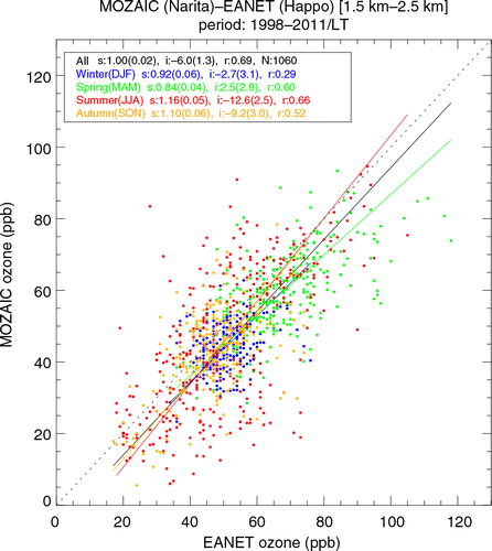
In summer, the data are more scattered than in other seasons, likely reflecting a different regime of synoptic-scale meteorology over Japan. Mt Happo is located in a rural area of western Japan, while Tokyo/Narita is located in eastern Japan and near the Tokyo metropolitan area. In summer, Japan is greatly influenced by the Asian Monsoon, but its influence is somewhat stronger in the east than in the west. It is interesting to note that the springtime data show a slope of 0.84, indicating that the O₃ concentration is 16% higher at Mt. Happo than that over Tokyo/Narita, likely reflecting a stronger influence from the continental outflow in western Japan (Tanimoto et al., 2005).

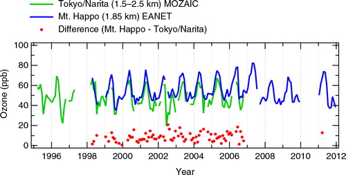
Figure 11 shows the time series data of monthly mean O₃ observed at Mt. Happo and those observed by the MOZAIC aircraft over Tokyo/Narita at the 1.5–2.5 km altitude level. These data are not concomitant. Also shown are the differences between these observations for the period from 1998 to 2006, when there are overlaps for the EANET observations at Mt. Happo and the MOZAIC observations over the Tokyo/Narita airport. Interestingly, the O₃ concentration at Mt. Happo tends to be higher than that over Tokyo/Narita. This feature appears to happen regardless of the season or year. The magnitude of the differences varies from 0 to 20 ppb, and the mean difference is 8.6 (±4.4) ppb for 79 monthly data pairs.

Fig. 11 Time series of monthly mean ozone observed at Mt. Happo and over Tokyo/Narita for the altitude of 1.5–2.5 km. The differences between two observations sites (Mt. Happo minus Tokyo/Narita) are also plotted.

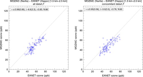
In Fig. 12, monthly mean O₃ data calculated from all the available data and from only concomitant data are compared for the MOZAIC aircraft observations over Tokyo/Narita against the EANET observations at Mt. Happo. These scatter plots show no essential differences due to the absence of the effects of diurnal cycles or samplings at fixed LT, unlike the case of Tsukuba. The correlations are strong, and the slopes are basically 1.0 within the 95% confidence limit. The correlation coefficient is 0.8, indicating that the variability can be controlled by 64%, which is reasonable. It should be noted that a bias of 3–6 ppb exists. This could be due to the fact that Mt. Happo is located in the west coast of Japan, which is subject to a stronger influence of continental outflow from Asia.

Fig. 12 Scatter plots of monthly mean ozone made of all (left) and concomitant (right) hourly data, at Mt. Happo and over Tokyo/Narita for the altitude of 1.5–2.5 km.

4. Concluding remarks

The assessment of tropospheric O₃ trends through observations and model reanalysis, and the resulting future predictions are crucial for policy makers in order to keep climate change in a range reasonable for human health and activity. Consequently, long-term ‘in-situ’ measurements on a global scale must reach the highest possible data quality to validate the chemistry-climate or CTMs and space-borne observations. To increase the available data sets and maybe create a single data set as global as possible for such validations, it is of particular interest to first check the consistency between the different data sets provided by different instrument techniques, different regions and different altitudes. There are differences not only in techniques and locations, but technical details including measurement uncertainties, the height of sampling inlet from the ground surface, LT of sampling, and the number of data used for daily/monthly averages are also different. This has been the motivation for the present analysis focusing on Europe and Japan with three types of measurements.

In the present work, we examined the consistency of tropospheric O₃ observations made using surface sites, sondes and regular aircraft, whose data are publicly available in global databases including WDCGG, WOUDC and MOZAIC-IAGOS. First, we compared O₃ measurements by sondes and surface monitoring. At Hohenpeissenberg, Tsukuba, and Syowa, where the WOUDC sonde launching and the WDCGG surface monitoring are made at the same site and by the same institutes, the effects of different geographical locations were found negligible. Hence, the comparisons inherently mean a diagnosis of two different observing sensors used in the individual monitoring systems (i.e. electro-chemical method for ozonesondes and UV absorption for surface monitoring). The need to apply CF to BM-sondes was clearly identified, while the application of CF did not have significant impacts on ECC-sondes and CI-sondes. The comparison of MOZAIC-IAGOS aircraft and WDCGG surface monitoring enabled us to exclusively examine the effects of the differences in location (i.e. the representativeness of the sites) for tropospheric O₃ observations, since UV absorption is commonly employed in these programmes. Depending on seasons and local meteorology, large disagreements were occasionally observed. However, this problem can be avoided by the effort to select regionally representative air masses by using in situ wind data of the MOZAIC-IAGOS observations. When associated with substantial diurnal variations, caution must be paid to avoid possible over- or underestimates by sondes launched at a fixed LT, in particular in warm seasons. Here, we found an 8% underestimate and a 70% overestimate by the sondes against the surface observations at HPB and TKB, respectively. At HPB, the sonde data were still lower than the surface data, pointing to a further ~10% bias caused by local conditions at the launching site.

In spite of numerous differences in techniques, geographic locations and sampling time, the monthly means that are often used for trend analysis and model validation exhibit a reasonable agreement with each other. However, monthly means calculated from concomitant observations show a better agreement among data from different platforms than monthly means calculated from all data. This information could be a valuable contribution to constructing robust data sets of tropospheric O₃ on global scales by utilising multiple databases, leading to an improvement of our capability to analyse climatology, seasonal cycles and long-term trends of tropospheric O₃.

Acknowledgements

We acknowledge the following data centres. For ozonesondes: the World Ozone and Ultraviolet Radiation Data Centre (WOUDC, www.woudc.org) operated by Environment Canada, Toronto, Ontario, Canada, under the auspices of the WMO; for surface data: the World Data Centre for Greenhouse Gases (WDCGG, www.gaw.kishou.go.jp/wdcgg) maintained by the Japan Meteorological Agency, Tokyo, Japan, in cooperation with the WMO. Ushuaia ozone data were provided by the Global Atmosphere Watch Station of Ushuaia, managed by the National Weather Service of Argentina (SMN), in agreement with the National Institute of Aerospace Technology of Spain (INTA) and the State Meteorological Agency of Spain (AEMet). The data at Tsukuba and Syowa were provided by Aerological Observatory and Office of Antarctica Observation, respectively, of Japan Meteorological Agency. The data at Egbert and Saturna were provided by Air Quality Research Branch, Environment Canada. The data at Hohenpeissenberg and Neuglobsow were provided by the German Meteorological Service and Federal Environmental Agency of Germany, respectively. The data at Izana were provided by the Meteorological State Agency of Spain, at Trinidad Head by NOAA, and at Cape Point by the South African Weather Service. We also acknowledge the strong support of the European Commission, Airbus, and the Airlines (Lufthansa, Air-France, Austrian, Air Namibia, Cathay Pacific, Iberia and China Airlines so far) who carry the MOZAIC or IAGOS equipment and perform the maintenance since 1994. MOZAIC is presently funded by INSU-CNRS (France), Météo-France, CNES, Université Paul Sabatier (Toulouse, France) and Research Center Jülich (FZJ, Jülich, Germany). IAGOS has been and is additionally funded by the EU projects IAGOS-DS and IAGOS-ERI. The MOZAIC-IAGOS data are available via CNES/CNRS-INSU Ether website www.pole-ether.fr.

We also thank the German Weather Service (Meteorological Observatory at Hohenpeissenberg), the National Space Development Agency of Japan and NASA (Wallops Island Flight Facility) for providing their data through the WOUDC. Funding for research was provided partly by the Global Environment Research Fund of the Ministry of the Environment, Japan (S-7-1 and 2-1505). H.T. thanks Kimiko Suto and Haruka Yamagishi at NIES for technical support, and Dr. Edit Nagy-Tanaka at NIES for editing the manuscript. We thank two anonymous reviewers for their valuable comments for improving the paper.

Notes

This paper is part of a Special Issue on MOZAIC/IAGOS in Tellus B celebrating 20 years of an ongoing air chemistry-climate research measurement from airbus commercial aircraft operated by an international consortium of countries. More papers from this issue can be found at http://www.tellusb.net

References

- Chang Y. S. , Carmichael G. R. , Kurita H. , Ueda H . The transport and formation of photochemical oxidants in central Japan. Atmos. Environ. 1989; 23(2): 363–393.
- Derwent R. G. , Simmonds P. G. , Manning A. J. , Spain T. G . Trends over a 20-year period from 1987 to 2007 in surface ozone at the atmospheric research station, Mace Head, Ireland. Atmos. Environ. 2007; 41: 9091–9098.
- Fuhrer J. , Skarby L. , Ashmore M . Critical levels of ozone effect in Europe. Environ. Pollut. 1997; 97: 91–106.
- Hassler B. , Petropavlovskikh I. , Staehelin J. , August T. , Bhartia P. K. , co-authors . Past changes in the vertical distribution of ozone – part 1: measurement techniques, uncertainties and availability. Atmos. Meas. Tech. 2014; 7: 1395–1427. DOI: http://dx.doi.org/10.5194/amt-7-1395-2014 .
- Jaffe D. , Price H. , Goldstein A. , Harris J . Increasing background ozone during spring on the west coast of North America. Geophys. Res. Lett. 2003; 30: 1613. DOI: http://dx.doi.org/10.1029/2003GL017024 .
- Lee S. , Akimoto H. , Nakane H. , Kurnosenko S. , Kinjo Y . Lower tropospheric ozone trend observed in 1989–1997 at Okinawa, Japan. Geophys. Res. Lett. 1998; 25: 1637–1640.
- Lelieveld J. , van Aardenne J. , Fischer H. , de Reus M. , Williams J. , co-authors . Increasing ozone over the Atlantic Ocean. Science. 2004; 304: 1483–1487.
- Liu G. , Tarasick D. W. , Fioletov V. E. , Sioris C. E. , Rochon Y. J . Ozone correlation lengths and measurement uncertainties from analysis of historical ozonesonde data in North America and Europe. J. Geophys. Res. 2009; 114: 04112. DOI: http://dx.doi.org/10.1029/2008JD010576 .
- Logan J. A . Trends in the vertical distribution of ozone: an analysis of ozonesonde data. J. Geophys. Res. 1994; 99(D12): 25553–25585.
- Logan J. A. , Megretskaia I. A. , Miller A. J. , Tiao G. C. , Choi D. , co-authors . Trends in the vertical distribution of ozone: a comparison of two analyses of ozonesonde data. J. Geophys. Res. 1999; 104: 26373–26399.
- Logan J. A. , Staehelin J. , Megretskaia I. A. , Cammas J.-P. , Thouret V. , co-authors . Changes in ozone over Europe: analysis of ozone measurements from sondes, regular aircraft (MOZAIC) and alpine surface sites. J. Geophys. Res. 2012; 117: 09301. DOI: http://dx.doi.org/10.1029/2011JD016952 .
- Marenco A. , Thouret V. , Nédélec P. , Smit H. , Helten M. , co-authors . Measurement of ozone and water vapor by Airbus in-service aircraft: the MOZAIC airborne program, an overview. J. Geophys. Res. 1998; 103(D19): 25631–25642. DOI: http://dx.doi.org/10.1029/98JD00977 .
- Morris G. A. , Labow G. , Akimoto H. , Takigawa M. , Fujiwara M. , co-authors . On the use of the correction factor with Japanese ozonesonde data. Atmos. Chem. Phys. 2013; 13: 1243–1260. DOI: http://dx.doi.org/10.5194/acp-13-1243-2013 .
- Naja M. , Akimoto H . Contribution of regional pollution and long-range transport to the Asia–Pacific region: analysis of long-term ozonesonde data over Japan. J. Geophys. Res. 2004; 109: 21306. DOI: http://dx.doi.org/10.1029/2004JD004687 .
- Network Center for EANET. Acid Deposition Monitoring Network in East Asia (EANET). 2007; Niigata: Network Center for EANET. 131–172. Data report 2006.
- Oltmans S. J. , Lefohn A. S. , Harris J. M. , Galbally I. , Scheel H. E. , co-authors . Long-term changes in tropospheric ozone. Atmos. Environ. 2006; 40: 3156–3173.
- Oltmans S. J. , Lefohn A. S. , Scheel H. E. , Harris J. M. , Levy H., II. , co-authors . Trends of ozone in the troposphere. Geophys. Res. Lett. 1998; 25: 139–142.
- Oltmans S. J. , Lefohn A. S. , Shadwick D. , Harris J. M. , Scheel H. E. , co-authors . Recent tropospheric ozone changes – a pattern dominated by slow or no growth. Atmos. Environ. 2013; 67: 331–351.
- Parrish D. D. , Lamarque J.-F. , Naik V. , Horowitz L. , Shindell D. T. , co-authors . Long-term changes in lower tropospheric baseline ozone concentrations: comparing chemistry-climate models and observations at northern midlatitudes. J. Geophys. Res. Atmos. 2014; 119: 5719–5736. DOI: http://dx.doi.org/10.1002/2013JD021435 .
- Parrish D. D. , Law K. S. , Staehelin J. , Derwent R. , Cooper O. , co-authors . Long-term changes in lower tropospheric baseline ozone concentrations at northern mid-latitudes. Atmos. Chem. Phys. 2012; 12: 11485–11504.
- Petzold A. , Thouret V. , Gerbig C. , Zahn A. , Brenninkmeijer C. A. M. , co-authors . Global-scale atmosphere monitoring by in-service aircraft – current achievements and future prospects of the European Research Infrastructure IAGOS. Tellus B. 2015; 67: 28452. DOI: http://dx.doi.org/10.3402/tellusb.v67.28452 .
- Saunois M. , Emmons L. , Lamarque J.-F. , Tilmes S. , Wespes C. , co-authors . Impact of sampling frequency in the analysis of tropospheric ozone observations. Atmos. Chem. Phys. 2012; 12: 6757–6773. DOI: http://dx.doi.org/10.5194/acp-12-6757-2012 .
- Shindell D. , Kuylenstierna J. C. I. , Faluvegi G. , Milly G. , Emberson L. , co-authors . Simultaneously mitigating near-term climate change and improving human health and food security. Science. 2012; 335: 183–189.
- Simmonds P. G. , Derwent R. G. , Manning A. L. , Spain G . Significant growth in surface ozone at Mace Head, Ireland, 1987–2003. Atmos. Environ. 2004; 38: 4769–4778.
- Smit H. G. J. , ASOPOS Panel . Quality Assurance and Quality Control for Ozonesonde Measurements in GAW. 2013. WMO/GAW Report No. 201, WMO, Geneva.
- Smit H. G. J. , Straeter W. , Johnson B. , Oltmans S. , Davies J. , co-authors . Assessment of the performance of ECC-ozonesondes under quasi-flight conditions in the environmental simulation chamber: insights from the Juelich Ozone Sonde Intercomparison Experiment (JOSIE). J. Geophys. Res. 2007; 112: 19306. DOI: http://dx.doi.org/10.1029/2006JD007308 .
- SPARC. SPARC-IOC-GAW Assessment of Trends in the Vertical Distribution of Ozone. 1998; Geneva: World Meteorological Organization. SPARC Report No. 1, WMO Global Ozone Research and Monitoring Project Report No. 43.
- Staehelin J. , Thudium J. , Buehler R. , Volz-Thomas A. , Graber W . Trends in surface ozone concentrations at Arosa (Switzerland). Atmos. Environ. 1994; 28: 75–87.
- Staufer J. , Staehelin J. , Stübi R. , Peter T. , Tummon F. , co-authors . Trajectory matching of ozonesondes and MOZAIC measurements in the UTLS – part 1: method description and application at Payerne, Switzerland. Atmos. Meas. Tech. 2013; 6: 3393–3406. DOI: http://dx.doi.org/10.5194/amt-6-3393-2013 .
- Staufer J. , Staehelin J. , Stübi R. , Peter T. , Tummon F. , co-authors . Trajectory matching of ozonesondes and MOZAIC measurements in the UTLS – part 2: application to the global ozonesonde network. Atmos. Meas. Tech. 2014; 7: 241–266. DOI: http://dx.doi.org/10.5194/amt-7-241-2014 .
- Stevenson D. S. , Young P. J. , Naik V. , Lamarque J.-F. , Shindell D. T. , co-authors . Tropospheric ozone changes, radiative forcing and attribution to emissions in the Atmospheric Chemistry and Climate Model Intercomparison Project (ACCMIP). Atmos. Chem. Phys. 2013; 13: 3063–3085. DOI: http://dx.doi.org/10.5194/acp-13-3063-2013 .
- Tanimoto H . Increase in springtime tropospheric ozone at a mountainous site in Japan for the period 1998–2006. Atmos. Environ. 2009; 43: 1358–1363.
- Tanimoto H. , Mukai H. , Sawa Y. , Matsueda H. , Yonemura S. , co-authors . Direct assessment of international consistency of standards for ground-level ozone: strategy and implementation toward metrological traceability network in Asia. J. Environ. Monit. 2007; 9: 1183–1193. DOI: http://dx.doi.org/10.1039/b701230f [PubMed Abstract].
- Tanimoto H. , Ohara T. , Uno I . Asian anthropogenic emissions and decadal trends in springtime tropospheric ozone over Japan: 1998–2007. Geophys. Res. Lett. 2009; 36: 23802. DOI: http://dx.doi.org/10.1029/2009GL041382 .
- Tanimoto H. , Sawa Y. , Matsueda H. , Uno I. , Ohara T. , co-authors . Significant latitudinal gradient in the surface ozone spring maximum over East Asia. Geophys. Res. Lett. 2005; 32: 21805. DOI: http://dx.doi.org/10.1029/2005GL023514 .
- Thouret V. , Cammas J.-P. , Sauvage B. , Athier G. , Zbinden R. , co-authors . Tropopause referenced ozone climatology and inter-annual variability (1994–2003) from the MOZAIC programme. Atmos. Chem. Phys. 2006; 6: 1033–1051. DOI: http://dx.doi.org/10.5194/acp-6-1033-2006 .
- Thouret V. , Marenco A. , Logan J. A. , Nédélec P. , Grouhel C . Comparisons of ozone measurements from the MOZAIC airborne program and the ozone sounding network at eight locations. J. Geophys. Res. 1998; 103: 695–720.
- Thouret V. , Petzold A . Observing the global atmosphere by instrumented passenger aircraft – the story of IAGOS. WMO Bull. 2014; 63(2): 19–21.
- Tilmes S. , Lamarque J.-F. , Emmons L. K. , Conley A. , Schultz M. G. , co-authors . Technical note: ozonesonde climatology between 1995 and 2011: description, evaluation and applications. Atmos. Chem. Phys. 2012; 12: 7475–7497. DOI: http://dx.doi.org/10.5194/acp-12-7475-2012 .
- Toohey M. , Hegglin M. I. , Tegtmeier S. , Anderson J. , Añel J. A. , co-authors . Characterizing sampling bias in the trace gas climatologies of the SPARC data initiative. J. Geophys. Res. Atmos. 2013; 118: 11847–11862. DOI: http://dx.doi.org/10.1002/jgrd.50874 .
- Tressol M. , Ordonez C. , Zbinden R. , Brioude J. , Thouret V. , co-authors . Air pollution during the 2003 European heat wave as seen by MOZAIC airliners. Atmos. Chem. Phys. 2008; 8: 2133–2150. DOI: http://dx.doi.org/10.5194/acp-8-2133-2008 .
- UNEP/WMO. Integrated Assessment of Black Carbon and Tropospheric Ozone: Summary for Decision Makers. 2011; Nairobi: UNON/Publishing Services Section.
- Van Dingenen R. , Dentener F. J. , Raes F. , Krol M. C. , Emberson L. , co-authors . The global impact of ozone on agricultural yields under current and future air quality legislation. Atmos. Environ. 2009; 43: 604–618.
- Voltz A. , Kley D . Evaluation of the Montsouris series of ozone measurements made in the nineteenth century. Nature. 1988; 332: 240–242.
- WHO. WHO Air Quality Guidelines for Particulate Matter, Ozone, Nitrogen Dioxide and Sulfur Dioxide. 2006; WHO, Geneva: Global update 2005.
- Wild O. , Akimoto H . Intercontinental transport of ozone and its precursors in a three-dimensional global CTM. J. Geophys. Res. 2001; 106: 27729–27744.
- WMO. WMO Global Atmosphere Watch (GAW) Strategic Plan: 2008–2015.
- Zbinden R. M. , Cammas J.-P. , Thouret V. , Nédélec P. , Karcher F. , co-authors . Mid-latitude tropospheric ozone columns from the MOZAIC program: climatology and interannual variability. Atmos. Chem. Phys. 2006; 6: 1053–1073.
- Zbinden R. M. , Thouret V. , Ricaud P. , Carminati F. , Cammas J.-P. , co-authors . Climatology of pure tropospheric profiles and column contents of ozone and carbon monoxide using MOZAIC in the mid-northern latitudes (24°N to 50°N) from 1994 to 2009. Atmos. Chem. Phys. 2013; 13: 12363–12388. DOI: http://dx.doi.org/10.5194/acp-13-12363-2013 .