Analysis of tropospheric ozone and carbon monoxide profiles over South America based on MOZAIC/IAGOS database and model simulations

Abstract

We analysed ozone and carbon monoxide profiles measured by commercial aircrafts from the MOZAIC/IAGOS fleet, during ascending and descending flights over Caracas, in Venezuela, from August 1994 to December 2009, over Rio de Janeiro, from 1994 to 2004 and from July 2012 to June 2013, and over São Paulo, in Brazil, from August 1994 to 2005. For ozone, results showed a clean atmosphere over Caracas presenting the highest seasonal mean in March, April and May. Backward trajectory analyses with FLEXPART, of case studies for which the measured concentrations were high, showed that contributions from local, Central and North America, the Caribbean and Africa either from anthropogenic emissions, biomass burning or lightning were possible. Satellite products as fire counts from MODIS, lightning flash rates from LIS, and CO and O₃ from Infrared Atmospheric Sounding Interferometer and wind maps at different levels helped corroborate previous findings. Sensitivity studies performed with the chemical transport model GEOS-Chem captured the effect of anthropogenic emissions but underestimated the influence of biomass burning, which could be due to an underestimation of GFEDv2 emission inventory. The model detected the contribution of lightning from Africa in JJA and SON and from South America in DJF, possibly from the northeast of Brazil. Over São Paulo and Rio de Janeiro, GEOS-Chem captured the seasonal variability of lightning produced in South America and attributed this source as the most important in this region, except in JJA, when anthropogenic emissions were addressed as the more impacting source of ozone precursors. However, comparison with the measurements indicated that the model overestimated ozone formation, which could be due to the convective parameterisation or the stratospheric influence. The highest ozone concentration was observed during September to November, but the model attributed only a small influence of biomass burning from South America, with no contribution of long-range transport from Africa.

• tropospheric ozone
• carbon monoxide
• MOZAIC/IAGOS
• air pollution
• GEOS-Chem
• FLEXPART
• South America
• biomass burning
• IASI

This paper is part of a Special Issue on MOZAIC-IAGOS in Tellus B celebrating 20 years of an ongoing air chemistry climate research measurements from airbus commerical aircraft operated by an international consortium of countries. More papers from this issue can be found at http://www.tellusb.net

1. Introduction

Tropospheric ozone (O₃) can act as a greenhouse effect gas; affect the oxidising capacity of the atmosphere; and be harmful to the human health, plants and material. Ashmore (2005) presented a review on the observed injuries caused by high ozone concentrations in crops and forests throughout the world. Visible injury to horticultural crops, for example, caused an impact on their economic value. Other reported injuries are the reduction on photosynthesis rate and the acceleration of leaf senescence. According to Curtis et al. (2006), emergency room visits due to respiratory and cardiovascular problems presented statistically significant correlation with ozone concentration near the surface.

Ozone formation in the troposphere is due to both natural and anthropogenic precursor sources. In the tropics, the main natural sources of ozone precursors are the tropical vegetation and microbial processes in soil (Guenther et al., 1995; Jaeglé et al., 2005), deep convection because of associated lightning, the last especially over the South Atlantic Ocean (Moxim and Levy, 2000; Martin et al., 2007; Sauvage et al., 2007a). Although forest vegetation is an important source of volatile organic compounds (VOCs) to the atmosphere, Lelieveld et al. (2008) proposed new pathways to the produced biogenic VOC, in the Amazon region, which maintains the atmospheric oxidation capacity without excess ozone formation, in a balanced cycle. According to Jaeglé et al. (2005), the largest soil emission is observed over tropical savanna and woodlands in Africa, during the rainy season.

Many studies conducted in South America identified biomass burning as the main source of tropospheric ozone with enhanced concentrations during August to November (Thompson et al., 1996; Kim and Newchurch, 1998; Galanter et al., 2000; Andreae and Merlet, 2001; Ziemke et al., 2009; Longo et al., 2010). In large cities as São Paulo and Rio de Janeiro, local urban pollution can also be an important source of ozone precursors (Andrade et al., 2012). Martins and Andrade (2008) identified vehicular emission as the main source of ozone precursors in the boundary layer of São Paulo Metropolitan Area.

Finally, dynamical atmospheric processes associated with cut-off lows either generated by convective erosion, turbulent mixing near the jet stream and tropopause folding influence stratosphere to troposphere exchange (STE), increasing the ozone concentration in the upper troposphere (Price and Vaughan, 1993; Scott et al., 2001; Thouret et al., 2006; Iwabe and Rocha, 2009; Pena-Ortiz et al., 2013).

Carbon monoxide (CO) presents an important role in the atmospheric chemistry, being a product of the photo-oxidation of methane and other VOCs. It represents the most important sink for the hydroxyl (OH) radical and is a precursor of tropospheric O₃ (Andreae et al., 2012). Over the tropics, the main sources are biomass burning, oxidation of methane and biogenic hydrocarbons, and fossil fuel contributions over megacities as, for example, São Paulo and Buenos Aires in South America (Holloway et al., 2000; Duncan et al., 2007; Alonso et al., 2010).

Taking advantage of the long-term flights performed by MOZAIC (Measurements of OZone, water vapour, carbon monoxide and nitrogen oxides by in-service Airbus aircraft; www.iagos.fr/mozaic; Marenco et al., 1998) and IAGOS (In-service Aircraft for a Global Observing System; www.iagos.org/; Petzold et al., 2015) projects over South America, we address the following questions: (1) can we observe seasonal and interannual variability of tropospheric ozone concentration measured over Caracas, São Paulo and Rio de Janeiro based on those flights? (2) in episodes with enhanced ozone or carbon monoxide concentrations, what were the main source regions of those pollutants? (3) how important are the influences of biomass burning and lightning from South America and Africa to the measured tropospheric ozone concentration? Besides the analysis of such database, modelling studies were also performed. This paper is organised as follows: in Section 2, the analysed database and the methodological approaches are discussed as well as a brief summary of the utilised models. In Section 3, we discuss the results and present the main conclusions in Section 4.

2. Data and methodology

2.1. General description of the measurements

In this study, we analysed vertical profiles of tropospheric ozone and carbon monoxide (up to 200 hPa) collected in the framework of the MOZAIC and IAGOS programmes. Data were measured during descending and ascending flight legs of commercial aircraft over Caracas (located at 10°30′N, 66°55′W), in Venezuela, Rio de Janeiro (22°48′S, 43°13′W) and São Paulo (23°26′S, 46°29′W), in Brazil, from 1994 to 2013, when available. Around Caracas, most of the data were collected in the afternoon and evening peaking at around 15:00–18:00 (local time; UTC–04:30), with very few flights between 00:00 and 12:00. Over Rio de Janeiro, ascending or descending flights were more frequent in the afternoon, between 15:00 and 18:00 (local time; UTC–03:00), with a second peak in the morning, between 06:00 and 09:00. Finally, flight schedule concentrated between 03:00–09:00 and 12:00–21:00 (local time; UTC–03:00), with a peak around 18:00–21:00, in São Paulo.

Ozone measurements were performed using a dual beam ultraviolet absorption instrument whose detection limit was 2 ppbv with an overall precision of±2 ppbv +2% (Thouret et al., 1998). Calibration procedures have been unchanged since the beginning of the programme. Instruments are laboratory calibrated before and after the flight periods, whose interval can vary between 6 and 18 months. Measurements are carried out only after takeoff and before landing to avoid contamination of the input line by deposition of organic compounds and dust while the aircraft is on the ground and subject to local pollution (Marenco et al., 1998). CO measurements started by the end of 2001, but over South America systematic measurements started only in 2003. CO is measured using a modified infrared filter correlation monitor as described in Nédélec et al. (2003). For a 30-s response time, the instruments accuracy is estimated at ±5 ppbv and±5% (Nédélec et al., 2003).

Flights over Caracas, Rio de Janeiro and São Paulo were rather irregular. In some periods, two profiles per day were available (one during descending and the other during ascending flights) or one profile on 1 d and another on the following day, in variable intervals such as every day or with only two flights per trimester. The flights to Caracas were interrupted in 2009, towards São Paulo in 2005, while to Rio de Janeiro, they stopped in 2004 and were reinitiated in July 2012. We included data up to June 2013 over Rio de Janeiro in this study. Samples collected over São Paulo and Rio de Janeiro were analysed together, since those locations are close to each other when compared to the horizontal spatial resolution of GEOS-Chem model.

2.2. Seasonal and interannual variability analyses of partial ozone column

Partial ozone column (POC), in Dobson units, was estimated at the following levels: from surface up to 900 hPa, from 900 to 700 hPa, from 700 to 500 hPa, from 500 to 200 hPa and from surface up to 200 hPa. Seasonal and interannual variability analyses of POC were performed, taking into account the temporal autocorrelation in time series as discussed by Saunois et al. (2012). Briefly, this correction is necessary since atmospheric data often do not satisfy the assumption of independence, increasing the error estimates. Thus, to do so, the lag-1 autoregressive coefficient for each layer was estimated according to Wilks (2006):

where is the sample mean considering the first N-1 data values and is the sample mean considering the N-1 final data in that time interval.

Using this coefficient, the effective sample size was estimated as

the variance and the SE of the sample mean, , were then given by

where s is the sample SD.

Next, to analyse the interannual variability of the seasonal mean, a global weighted mean for each season was determined, considering all the estimated means. It is important to notice that the mean for each season, in a particular year, was estimated only if the effective size N _eff≥6, assuming that, effectively, at least two data values were available per month. The global seasonal weighted mean was estimated as

where is each seasonal mean estimated for every available year. The weights were calculated by

and the variance of the weighted mean was

Finally, the seasonal mean for each year was compared to the global seasonal mean, through the standard Gaussian z (Wilks, 2006):

If the numerator was more than about twice as large as the denominator in absolute value, the null hypothesis was rejected at the 5% level for a two-sided test. Thus, seasonal means for which z>2 were highlighted and classified as polluted when compared to the global mean.

2.3. FLEXPART and GEOS-Chem models

To identify the origin of air masses with enhanced ozone or CO mixing ratios, back-trajectories using FLEXPART (Flexible Particle Dispersion Model) version 9.0 were calculated. Layers with concentrations higher than 40 ppbv for ozone or 200 ppbv for CO were analysed. The adopted threshold for ozone was based on the lowest seasonal mean mixing ratio at all levels, over each city, of about 40 ppbv or less (see Figs. 1 and 2 in Section 3). Thus, layers with mixing ratio above this value were considered polluted and further investigated. For CO, the condition of >200 ppbv mixing ratio was observed only in the planetary boundary layer (PBL) of Caracas. Over the other two cities, the largest megacities of Brazil, values above this threshold were observed rarely and only close to the surface. FLEXPART is a Lagrangian particle dispersion model derived from FLEXTRA, a kinematic trajectory model, as detailed by Stohl et al. (2005). The model calculates trajectories of thousands of particles released from three-dimensional boxes either in backward or in forward mode. In this study, the boxes were defined along every MOZAIC/IAGOS flight track with 0.1°×0.1° and 0.1 hPa resolutions in the horizontal and vertical, respectively. As in Stohl et al. (2001) and Huntrieser et al. (2007), we run in backward mode for up to 14 d in the past, to allow better coverage. The latter is justified because when ozone is lifted to the free troposphere, it can last for days to weeks (Jenkins and Ryu, 2004). Carbon monoxide lifetime in the atmosphere varies between a week and 2 months (Edwards et al., 2003).

Fig. 1 Seasonal mean profile of carbon monoxide (on the left) and ozone (on the right) from the surface up to 200 hPa based on MOZAIC/IAGOS flight measurements performed during landing and taking off at Caracas, averaged over the period August 1994 to March 2009. Shading interval represents 1 SD and shows the variability of the data.

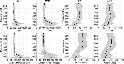
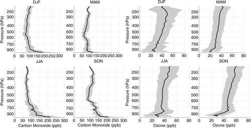
Fig. 2 Seasonal mean profile of carbon monoxide (on the left) and ozone (on the right) from the surface up to 200 hPa based on MOZAIC/IAGOS flight measurements performed during landing and taking off at Rio de Janeiro and São Paulo over the period from August 1994 to December 2012. Shading interval represents 1 SD and shows the variability of the data.

The model is driven by wind fields provided by the European Centre for Medium-range Weather Forecast (ECMWF) with a temporal resolution of 3 hours (analyses at 00:00, 06:00, 12:00, 18:00 UTC; forecasts at 03:00, 09:00, 15:00, 21:00 UTC) and with horizontal resolution of 32 km. The model output refers to the time, in seconds, the released particles spent in each output grid box before reaching the flight segment under analysis. We adopted 0.5° latitude×0.5° longitude×500 m altitude for a grid box. This residence time was further normalised, dividing it to the 14 d, the full integration time adopted to calculate the back trajectories. Seasonal maps of the normalised residence time, in percent, were constructed showing the distribution of air mass originating from low (<700 hPa), intermediate (from 700 to 380 hPa) and high altitudes (from 380 to ~60 hPa) arriving at flight layers with enhanced concentrations located in low (below 700 hPa), mid (from 650 to 380 hPa) and upper troposphere (from 380 hPa up to the maximum flight altitude at ~200 hPa). The main goal here is to verify if the air masses with enhanced concentrations (i.e. highly polluted) follow a very well-defined path and have similar emission sources at a seasonal basis.

To identify the relative importance of distinct ozone precursor emissions in the tropospheric ozone burden, over the studied cities, numerical modelling simulations were performed with a climatological perspective. The off-line global chemical transport model (CTM) GEOS-Chem (Bey et al., 2001), version 9-01-01, was used, driven by assimilated meteorological data from the Goddard Earth Observing System (GEOS-5) of the NASA Global Modeling and Assimilation Office, with a horizontal resolution of 2° latitude×2.5° longitude. In GEOS-Chem, biomass burning GFED2 (Global Fire Emissions Database version 2) inventory with monthly resolution was used. Due to the lack of a regional inventory for anthropogenic emission over South America, EDGAR v.4.1 for global anthropogenic emission was used. It provides annual global emissions of greenhouse gases and ozone precursors on a 1°×1° horizontal resolution. We also used the regional emission inventories: EMEP for Europe, CAC for Canada, BRAVO for Mexico, Streets for Southeast Asia, EPA/NEI99 with ICARTT modification for North America, all anthropogenic inventories scaled for the year 2005. The default biogenic emission was MEGAN v2.1. Detailed information on the emission inventories can be consulted on www.acmg.seas.harvard.edu/geos/doc/archive/man.v9-01-01/index.html. Runs with secondary organic aerosol (SOA) formation were performed. Sensitivity analysis (not presented) showed that runs without SOA formation caused more overestimation of tropospheric O₃ than considering SOA when compared to the measured climatology, particularly during the peak of the South American burning season, that is, from September to November (SON). Six distinct simulations were performed allowing a 6-month period spin-up: the control run considering all the emission sources and areas (ALL); considering no biomass burning NO _x emission from Africa (box centred at coordinates 32°S–34°N; 25°W–50°E) (NoBB-AF); considering no lightning NO _x from Africa (NoLight-AF); zeroing biomass burning NO _x emission in South America (54°S–12°N; 82.5°W–25°W) (NoBB-SA); considering no lightning NO _x emission in South America (NoLight-SA); and turning off all sources of anthropogenic emissions (NoAnth). Runs for the year 2009 were compared with climatological observed data for São Paulo and Rio de Janeiro together, given the model horizontal resolution. For Caracas, observation and simulation results were compared for the year 2007. We selected those years for comparison first due to the availability of meteorological data for the runs (2004–2012). For Caracas, the year with maximum observations available was 2003, followed by 2007 (37 profiles in December, January and February – DJF; 26 in March, April, May – MAM; 24 in June, July, August – JJA, but only 10 in September, October and November – SON), which motivated our choice in this case. Over São Paulo and Rio de Janeiro, the model runs for 2009 best represented the mean climatological profiles, which, in principle, could help diagnose the main sources of ozone precursors to the region. For example, using the year 2007, both ozone and carbon monoxide profiles from the model systematically overestimated observations in all the seasons, the difference reaching > 45 ppb for CO at about 750 hPa and 30 ppb for O₃ at 500 hPa in SON.

Given the low horizontal resolution of the model and the location of Caracas at the Venezuelan coast, emission inventories can present higher uncertainty in the region due to the land/water mask, affecting modelled concentration particularly in the PBL. Also, local circulation as sea breeze could also interfere in the model versus observation comparison.

Finally, the comparison between GEOS-Chem results and the measurements above 220 hPa for São Paulo and Rio de Janeiro, and 280 hPa for Caracas, must be analysed with caution. Above those thresholds, 37% of the flights over Rio de Janeiro, 23% of the flights over São Paulo and 42% over Caracas were outside the horizontal grid resolution of the model.

2.4. Satellite products: fire counts, mean flash rate data, carbon monoxide and ozone

To help interpret the results, satellite fire counts per pixel and mean flash rate from lightning data were also used. Monthly archives of fire counts from MODIS (Moderate Resolution Imaging Spectroradiometer) on board Terra satellite with 1°×1° horizontal resolution from January 2002 to December 2012 were used to create seasonal maps in the region limited by latitude from 60°S to 60°N and longitude from 120°W to 40°E, covering South and Central Americas and parts of North America and Africa. Data were downloaded from www.mirador.gsfc.nasa.gov/.

Lightning seasonal maps were created for the same area using monthly climatology of flash rate data (# flashes km⁻² month⁻¹) from LIS (Lightning Imaging Sensor) on board TRMM (Tropical Rainfall Measuring Mission) with 0.5°×0.5° horizontal resolution from January 2008 to December 2012. Data were downloaded from www.thunder.nsstc.nasa.gov/.

Seasonal maps of CO, O₃ and horizontal wind vectors were generated to have a broader view of CO and O₃ distributions and a better understanding of their transport pathways, covering South American and African continents in the same area defined previously. For CO and O₃, we used retrieved data from the Infrared Atmospheric Sounding Interferometer (IASI) on board the MetOp-A satellite (George et al., 2009; Turquety et al., 2009). The Metop-A/IASI is a thermal infrared sensor that provides a global coverage twice daily. IASI enables us to quantify the atmospheric content of a number of chemicals such as CO (De Wachter et al., 2012) and O₃ (Barret et al., 2011). The O₃ data used in the present study were retrieved from IASI radiances using the Software for a Fast Retrieval of IASI Data (SOFRID) described in Barret et al. (2011). IASI-SOFRID O₃ data were validated on the global scale with ozonesonde data (Barret et al., 2011; Dufour et al., 2012), while CO data were validated with MOZAIC-IAGOS data (De Wachter et al., 2012). The retrieved tropospheric profiles contain approximately two independent pieces of information corresponding to pressure levels of roughly 520 and 220 hPa for O₃ (Barret et al., 2011) and of roughly 800 and 220 hPa for CO (De Wachter et al., 2012), the ones adopted in this study. The maps were generated averaging all available data from 2008 to 2012 for day and nighttime overpasses on 1°×1° grids. The seasonal maps of horizontal wind vectors at 800, 500 and 225 hPa levels were produced at 0.25°×0.25° horizontal resolution with data from the ECMWF Global Reanalysis ERA Interim monthly means of daily means for the same period as IASI-SOFRID maps.

Episodes, for which we identified stratospheric intrusions, were excluded from this study. Such episodes identification was based on the analysis of potential vorticity (PV) anomalies as suggested by Thouret et al. (2006). The authors considered pressure intervals of ±15 hPa around atmospheric layer with PV higher or equal to 2 PVU (1 PVU = 10⁻⁶ K m² kg⁻¹ s⁻¹) to classify such air mass as stratosphere contaminated. At the analysed cities latitudes, the tropopause layer is located above 13 km (15–17 km) (Homeyer and Bowman, 2013). The frequency of occurrence of those episodes over South America can be found in Yamasoe et al. (2015).

3. Results and discussion

3.1. Seasonal and interannual variability of ozone and CO concentrations

Figure 1 shows the mean seasonal vertical profiles of carbon monoxide and ozone over Caracas for the period of August 1994 to March 2009. Carbon monoxide presented the highest mean concentrations in MAM, in the PBL, with values above 170–180 ppbv from the ground to 750 hPa. Concentrations as high as 400 ppbv were measured in this season, in years 2003 and 2007, which contributed to raise the mean concentration in this layer. Aloft, the mean CO mixing ratio was approximately constant, around 100 ppbv, in the four seasons. For ozone, the average profiles presented two peaks, one in the boundary layer and a more intense in the mid-troposphere. Again MAM presented the highest mean ozone concentrations and was the only season with mean concentration above 30 ppbv in the PBL.

Table 1(a–d) presents seasonal mean POC values at four distinct layers (from the surface up to 900 hPa, 900–700 hPa, 700–500 hPa and 500–200 hPa) and also integrated from the surface up to 200 hPa, for each year estimated over Caracas. As observed in Fig. 1, MAM is the season with the highest O₃ mean concentration, leading to more than 24 DU when integrated from the surface up to 200 hPa. In the other seasons, mean value is around 20 DU, indicating a rather clean atmosphere in terms of tropospheric ozone column. According to the z estimation, statistically significantly mean values higher than the global seasonal mean (z≥2) were observed in December, January and February (DJF), in the year 2006 at the layer from 500 to 200 hPa, in 2007 close to the surface and in 2008 from 700 to 500 hPa. In MAM, only at the layer closest to the surface, the mean POC in 2003 and 2007 was significantly higher than the global mean, which coincided with the period when the highest CO concentration was observed in the PBL. Finally, in SON, those values were observed only in 2004 and 2006, and again closest to the surface. As discussed in the Section 2, the number of effective (N _eff) sample was reduced due to auto-correlation ( ρ ₁>0 in the tables), and seasonal means for years with N _eff<6 were disregarded. Thus, due to the lack of enough data, no trend analysis for POC was possible.

Table 1. Seasonal mean of partial ozone column, in DU, for each year and different altitudes and respective SE corrected for autocorrelation in time

(a) December, January and February (DJF) – Caracas
Surface to 900 hPa (ρ 1=0.445)
Year	(DU)	s mean (DU)	N	N eff	z
1995	0.85	0.24	32	12	−1.56
1997	0.73	0.25	31	12	−1.95
2006	1.49	0.27	16	6	0.77
2007	2.52	0.33	33	13	3.68
2008	1.36	0.23	29	11	0.40
2009	1.21	0.18	47	18	−0.25
	1.26	0.10
900–700 hPa (ρ 1=0.572)
Year	(DU)	s mean (DU)	N	N eff	z
1995	4.07	0.47	32	9	−0.10
1997	2.65	0.35	32	9	−3.79
2007	5.20	0.40	33	9	2.51
2008	4.59	0.38	32	9	1.13
2009	4.29	0.30	56	15	0.51
	4.12	0.16
700–500 hPa (ρ 1=0.570)
Year	(DU)	s mean (DU)	N	N eff	z
1995	4.82	0.29	32	9	−1.63
1997	4.69	0.33	32	9	−1.80
2007	5.57	0.31	33	9	0.70
2008	6.23	0.38	32	9	2.20
2009	5.60	0.27	57	16	0.87
	5.33	0.14
500–200 hPa (ρ 1=0.440)
Year	(DU)	s mean (DU)	N	N eff	z
1995	6.85	0.29	30	12	−2.62
1997	7.04	0.33	28	11	−1.81
2006	9.32	0.54	15	6	2.93
2007	8.10	0.37	27	10	1.06
2008	8.19	0.38	26	10	1.28
2009	7.92	0.25	50	19	0.86
	7.68	0.13
Surface to 200 hPa (ρ 1=0.557)
Year	(DU)	s mean (DU)	N	N eff	z
1995	16.74	0.60	30	9	−2.75
1997	14.89	0.59	27	8	−5.69
2007	21.93	0.70	26	7	4.52
2008	20.60	0.65	23	7	2.93
2009	19.39	0.47	40	11	1.55
	18.55	0.26
(b) March, April and May (MAM) – Caracas
Surface to 900 hPa (ρ 1=0.445)
Year	(DU)	s mean (DU)	N	N eff	z
1995	0.60	0.27	16	6	−3.59
1996	1.27	0.32	16	6	−1.12
1999	1.38	0.23	21	8	−1.05
2000	1.61	0.35	16	6	−0.08
2003	2.12	0.21	51	20	2.01
2006	1.88	0.26	22	8	0.85
2007	3.24	0.45	18	7	3.44
2008	1.83	0.43	16	6	0.41
	1.65	0.10
900–700 hPa (ρ 1=0.572)
Year	(DU)	s mean (DU)	N	N eff	z
1999	5.10	0.50	21	6	−1.45
2003	6.15	0.37	51	14	0.52
2006	6.31	0.50	22	6	0.70
	5.91	0.26
700–500 hPa (ρ 1=0.570)
Year	(DU)	s mean (DU)	N	N eff	z
2003	6.67	0.36	52	14	−0.35
2006	7.34	0.58	22	6	0.79
2007	6.75	0.53	21	6	−0.13
	6.83	0.27
500–200 hPa (ρ 1=0.440)
Year	(DU)	s mean (DU)	N	N eff	z
1999	9.64	0.62	20	8	1.34
2000	7.81	0.46	16	6	−1.99
2003	9.35	0.38	46	18	1.37
2006	9.80	0.59	20	8	1.66
2007	8.64	0.44	20	8	−0.29
2008	9.22	0.42	15	6	0.97
2009	7.44	0.46	15	6	−2.71
	8.78	0.17
Surface to 200 hPa (ρ 1=0.557)
Year	(DU)	s mean (DU)	N	N eff	z
2003	24.25	0.62	45	13	−0.37
2006	25.25	0.96	20	6	0.65
	24.54	0.52
(c) June, July and August (JJA) – Caracas
Surface to 900 hPa (ρ 1= 0.445)
Year	(DU)	s mean (DU)	N	N eff	z
1999	1.84	0.30	20	8	0.65
2000	1.00	0.22	20	8	−2.59
2003	1.60	0.16	93	36	−0.15
2006	2.37	0.39	20	8	1.82
2007	2.30	0.35	24	9	1.82
2008	1.88	0.41	15	6	0.58
	1.63	0.10
900–700 hPa (ρ 1=0.572)
Year	(DU)	s mean (DU)	N	N eff	z
2003	3.67	0.23	93	25	−0.40
2007	4.14	0.39	24	7	0.80
	3.79	0.20
700–500 hPa (ρ 1=0.570)
Year	(DU)	s mean (DU)	N	N eff	z
2003	5.33	0.24	93	25	0.07
2007	5.21	0.46	24	7	−0.17
	5.30	0.21
500–200 hPa (ρ 1=0.440)
Year	(DU)	s mean (DU)	N	N eff	z
1999	10.01	0.63	18	7	1.19
2000	7.81	0.57	19	7	−2.35
2003	9.35	0.28	80	31	0.36
2007	9.62	0.52	20	8	0.71
2008	9.07	0.49	15	6	−0.29
	9.22	0.20
Surface to 200 hPa (ρ 1=0.557)
Year	(DU)	s mean (DU)	N	N eff	z
2003	19.92	0.41	80	23	−0.58
2007	21.29	0.75	20	6	1.26
	20.24	0.36
(d) September, October and November (SON) – Caracas
Surface to 900 hPa (ρ 1=0.445)
Year	(DU)	s mean (DU)	N	N eff	z
1994	0.87	0.22	41	16	−2.39
1995	0.44	0.27	16	6	−3.50
2003	2.01	0.39	22	8	1.34
2004	2.51	0.35	22	8	2.86
2006	2.24	0.29	37	14	2.51
2008	1.86	0.29	28	11	1.26
	1.47	0.12
900–700 hPa (ρ 1=0.572)
Year	(DU)	s mean (DU)	N	N eff	z
1994	2.58	0.31	41	11	−3.56
2003	4.27	0.42	22	6	0.87
2004	4.81	0.50	22	6	1.78
2006	4.57	0.39	36	10	1.64
2008	4.34	0.43	33	9	1.01
	3.86	0.18
700–500 hPa (ρ 1=0.570)
Year	(DU)	s mean (DU)	N	N eff	z
1994	4.40	0.32	41	11	−1.33
2003	4.89	0.44	22	6	0.02
2004	5.22	0.36	22	6	0.86
2006	5.42	0.38	37	10	1.33
2008	4.71	0.31	33	9	−0.51
	4.88	0.16
500–200 hPa (ρ 1=0.440)
Year	(DU)	s mean (DU)	N	N eff	z
1994	8.57	0.35	41	16	−0.61
1995	7.59	0.48	16	6	−2.41
2003	10.38	0.55	19	7	2.73
2004	9.31	0.50	21	8	0.92
2006	9.84	0.38	27	10	2.45
2008	7.76	0.39	27	10	−2.48
	8.81	0.17
Surface to 200 hPa (ρ 1=0.557)
Year	(DU)	s mean (DU)	N	N eff	z
1994	16.43	0.60	40	11	−4.53
2004	22.01	0.65	21	6	3.32
2006	21.68	0.74	25	7	2.59
2008	18.98	0.78	22	6	−0.69
	19.57	0.34

Also shown the available number of vertical profiles from MOZAIC/IAGOS programmes in Caracas, Venezuela, the effective number of samples, the standard Gaussian z, the lag-1 autoregressive coefficient in parentheses and, on the last line for each layer, the global seasonal mean. Values in bold indicate values statistically above the global mean at the 5% significance level.

In Fig. 2, the mean seasonal profiles of CO and ozone concentrations measured over São Paulo and Rio de Janeiro, from August 1994 to December 2012, are presented. Carbon monoxide mean concentrations were higher closer to the surface, similar to Caracas, presenting high values (>100 ppb) up to about 600 hPa, above which it was almost constant with height, except in SON when a second peak could be observed between 350 and 250 hPa. This season also presented the highest mean concentration near the surface, followed by JJA. The main sources of CO in this region are local urban emission, particularly from fossil fuel combustion. However, in SON biomass burning contribution is also possible.

In the case of O₃ concentration, the mean values increased with altitude in the four seasons. Since stratospheric events were filtered in this study, other factors might explain this behaviour. According to Jacob et al. (1996), this could be due to the fact that above 6 km (~500 hPa), photochemistry changes from a net sink to a net source of ozone, which depends on the NO _x concentration. Also, São Paulo and Rio de Janeiro are located at the edge of the region over the Atlantic Ocean where ozone maximises in the mid-troposphere all year round.

The ozone mean concentration was below 30 ppbv in DJF and MAM close to the surface, reaching a maximum of about 50 ppbv around 300–250 hPa in DJF. Higher mean concentrations were observed in SON and varied between 40 and 55 ppbv, except at the levels closer to the surface where lower concentrations were observed as in the other seasons. In JJA and SON, a second peak was observed, between 900 and 750 hPa, in the former season, and less defined in the last, going from ~900 to 600 hPa. Ozone presented higher variability especially in DJF at higher altitudes, which could be due to updraft by convective systems.

Results for POC analysis at São Paulo and Rio de Janeiro are presented in Table 2(a–d). In this region, higher POC values from surface up to 200 hPa were observed in SON, reaching 29.9±1.0 DU in 2012, while the lowest global mean was observed during MAM. Note that for all the seasons, the more recent available mean POC was statistically significantly higher than the global mean season, at 95% level, with z systematically above 2, when integrated from the surface up to 200 hPa. This gives an indication of a possible tendency of increasing concentrations from year to year, but not linearly.

Table 2. Seasonal mean of partial ozone column, in DU, for each year and different altitudes and respective SE corrected for autocorrelation in time

(a) December, January and February (DJF) – Rio de Janeiro and São Paulo
Surface to 900 hPa (ρ 1=0.151)
Year	(DU)	s mean (DU)	N	N eff	z
1995	1.42	0.28	30	22	1.85
1996	0.74	0.16	46	34	−0.85
1997	0.59	0.10	92	68	−2.52
1998	1.42	0.17	84	62	2.85
1999	1.40	0.33	20	15	1.55
2000	0.69	0.25	11	8	−0.77
2013	1.61	0.27	12	9	2.64
	0.89	0.07
900–700 hPa (ρ 1=0.491)
Year	(DU)	s mean (DU)	N	N eff	z
1995	4.50	0.39	32	11	0.46
1996	4.33	0.35	55	19	0.06
1997	3.76	0.23	93	32	−2.05
1998	4.96	0.29	83	28	2.03
1999	4.53	0.40	23	8	0.52
	4.31	0.14
700–500 hPa (ρ 1=0.495)
Year	(DU)	s mean (DU)	N	N eff	z
1995	5.70	0.46	25	8	0.29
1996	5.62	0.35	48	16	0.14
1997	4.95	0.26	74	25	−2.04
1998	5.77	0.28	69	23	0.66
1999	6.48	0.44	23	8	2.00
2013	5.60	0.45	19	6	0.07
	5.56	0.14
500–200 hPa (ρ 1=0.296)
Year	(DU)	s mean (DU)	N	N eff	z
1995	8.16	0.53	17	9	−2.28
1996	9.24	0.42	34	18	−0.39
1997	9.60	0.34	49	27	0.48
1998	9.54	0.32	44	24	0.33
1999	10.24	0.43	20	11	1.79
2013	8.82	0.60	16	9	−0.96
	9.42	0.17
Surface to 200 hPa (ρ 1=0.371)
Year	(DU)	s mean (DU)	N	N eff	z
1995	20.58	0.86	15	7	0.56
1996	19.68	0.68	27	12	−0.53
1997	18.53	0.52	45	21	−2.62
1998	20.38	0.55	44	20	0.49
1999	22.54	0.71	17	8	3.25
	20.07	0.28
(b) March, April and May (MAM) – Rio de Janeiro and São Paulo
Surface to 900 hPa (ρ 1=0.151)
Year	(DU)	s mean (DU)	N	N eff	z
1996	0.74	0.14	56	41	−0.31
1997	0.72	0.10	88	65	−0.61
1998	1.12	0.17	67	49	1.82
1999	0.73	0.17	37	27	−0.31
2000	1.05	0.30	11	8	0.84
2006	0.66	0.27	8	6	−0.50
	0.79	0.06
900–700 hPa (ρ 1=0.491)
Year	(DU)	s mean (DU)	N	N eff	z
1996	4.10	0.28	65	22	−0.57
1997	4.48	0.23	93	32	0.77
1998	4.00	0.24	68	23	−0.99
1999	4.60	0.33	39	13	0.91
	4.28	0.13
700–500 hPa (ρ 1=0.495)
Year	(DU)	s mean (DU)	N	N eff	z
1996	4.45	0.25	55	19	−1.16
1997	4.79	0.20	74	25	0.07
1998	4.59	0.26	57	19	−0.64
1999	5.43	0.30	39	13	2.05
	4.77	0.12
500–200 hPa (ρ 1=0.296)
Year	(DU)	s mean (DU)	N	N eff	z
1996	7.16	0.39	28	15	−0.88
1997	7.45	0.25	51	28	−0.29
1998	7.09	0.34	38	21	−1.19
1999	8.74	0.33	32	17	3.34
2013	6.81	0.46	11	6	−1.49
	7.53	0.15
Surface to 200 hPa (ρ 1=0.371)
Year	(DU)	s mean (DU)	N	N eff	z
1996	15.68	0.58	24	11	−2.67
1997	17.14	0.34	48	22	−0.47
1998	16.43	0.52	38	17	−1.62
1999	19.55	0.47	30	14	4.26
	17.34	0.22
(c) June, July and August (JJA) – Rio de Janeiro and São Paulo
Surface to 900 hPa (ρ 1=0.151)
Year	(DU)	s mean (DU)	N	N eff	z
1996	1.07	0.15	69	51	−1.63
1997	1.41	0.15	80	59	0.32
1998	1.41	0.27	18	13	0.19
1999	1.22	0.21	34	25	−0.60
2003	1.80	0.19	9	7	2.13
	1.35	0.08
900–700 hPa (ρ 1=0.491)
Year	(DU)	s mean (DU)	N	N eff	z
1996	5.11	0.24	74	25	−1.56
1997	5.54	0.24	84	29	−0.03
1998	6.36	0.48	21	7	1.61
1999	6.21	0.40	35	12	1.58
	5.55	0.15
700–500 hPa (ρ 1=0.495)
Year	(DU)	s mean (DU)	N	N eff	z
1996	5.24	0.25	59	20	−0.04
1997	5.31	0.21	68	23	−0.03
1998	6.36	0.48	24	8	0.08
1999	6.32	0.33	34	11	0.10
	5.56	0.14
500–200 hPa (ρ 1=0.296)
Year	(DU)	s mean (DU)	N	N eff	z
1996	9.01	0.35	39	21	0.39
1997	7.99	0.30	43	23	−2.49
1998	10.18	0.52	16	9	2.38
1999	9.31	0.35	28	15	1.12
	8.86	0.18
Surface to 200 hPa (ρ 1=0.371)
Year	(DU)	s mean (DU)	N	N eff	z
1996	20.12	0.47	37	17	−2.02
1997	19.99	0.42	38	17	−2.46
1998	25.27	0.87	12	6	4.52
1999	22.84	0.51	27	12	2.91
	21.19	0.25
(d) September, October and November (SON) – Rio de Janeiro and São Paulo
Surface to 900 hPa (ρ 1=0.151)
Year	(DU)	s mean (DU)	N	N eff	z
1994	1.61	0.20	43	32	2.22
1995	1.27	0.34	10	7	0.39
1996	0.73	0.13	69	51	−2.74
1997	1.34	0.16	72	53	1.18
1998	0.93	0.25	16	12	−0.76
1999	1.03	0.22	33	24	−0.46
2012	3.08	0.45	13	10	4.26
	1.13	0.08
900–700 hPa (ρ 1=0.491)
Year	(DU)	s mean (DU)	N	N eff	z
1994	6.86	0.35	53	18	0.35
1995	6.47	0.54	25	9	−0.46
1996	6.29	0.30	68	23	−1.30
1997	6.97	0.31	73	25	0.69
1998	6.36	0.56	17	6	−0.64
1999	7.46	0.46	38	13	1.50
	6.73	0.16
700–500 hPa (ρ 1=0.495)
Year	(DU)	s mean (DU)	N	N eff	z
1994	7.45	0.30	40	14	0.50
1995	6.58	0.42	22	7	−1.63
1996	6.90	0.30	57	19	−1.21
1997	7.10	0.27	62	21	−0.63
1998	7.85	0.45	18	6	1.20
1999	7.80	0.28	38	13	1.64
	7.29	0.13
500–200 hPa (ρ 1=0.296)
Year	(DU)	s mean (DU)	N	N eff	z
1994	12.30	0.48	26	14	1.56
1995	10.38	0.60	15	8	−1.79
1996	11.38	0.39	35	19	−0.30
1997	11.07	0.38	35	19	−1.04
1998	11.24	0.57	15	8	−0.44
1999	11.94	0.42	32	17	0.96
2012	12.05	0.54	15	8	0.95
	11.50	0.17
Surface to 200 hPa (ρ 1=0.371)
Year	(DU)	s mean (DU)	N	N eff	z
1994	28.66	0.78	19	9	2.04
1996	25.27	0.57	35	16	−2.73
1997	25.64	0.56	35	16	−2.15
1998	26.45	0.77	13	6	−0.65
1999	28.31	0.53	30	14	2.24
2012	29.90	1.01	12	6	2.80
	26.98	0.27

Also shown the available number of vertical profiles from MOZAIC/IAGOS Programs in São Paulo and Rio de Janeiro, Brazil, the effective number of samples, the standard Gaussian z, the lag-1 autoregressive coefficient in parentheses and, on the last line for each layer, the global seasonal mean. Values in bold indicate values statistically above the global mean at the 5% significance level.

3.2. Air mass origin of polluted cases according to back-trajectory analysis

In Figs. (3–6), longer residence times result from higher contributions of air masses from the corresponding layer. In general, the highest contributing air mass corresponds to the ones traveling at the same altitude as the layer under analysis. This means, for instance, that contribution from the PBL to the upper troposphere is less frequent than to the PBL itself. We will first discuss the results for Caracas, located to the north of the black dashed lines in the figures.

Fig. 3 Origin of air mass based on FLEXPART 14-d back trajectories for cases whose flight layers presented ozone mixing ratios above 40 ppbv over Caracas, Rio de Janeiro or São Paulo in DJF. Colours represent the percent of residence time (or normalised residence time in percent). The columns correspond to flight layers: low troposphere (below 700 hPa) on the left; medium troposphere (between 650 and 380 hPa) on the middle; and upper troposphere (380–180 hPa) on the right panel, while rows correspond to the layers of air mass origin: low troposphere (below 700 hPa) at the top; mid-troposphere (700 to 380 hPa) on the second line and from higher altitudes (380 to ~60 hPa) at the bottom panels. The black dashed lines separate trajectories for Caracas from the ones for São Paulo or Rio de Janeiro.

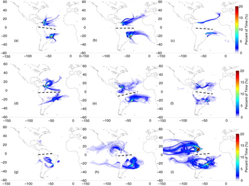
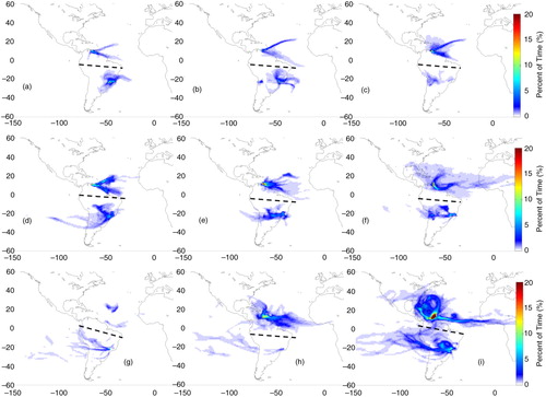
Fig. 4 Origin of air mass based on FLEXPART 14-d back trajectories for cases whose flight layers presented ozone mixing ratios above 40 ppbv over Caracas, Rio de Janeiro or São Paulo in MAM. Colours represent the percent of residence time (or normalised residence time in percent). The columns correspond to flight layers: low troposphere (below 700 hPa) on the left; medium troposphere (between 650 and 380 hPa) on the middle; and upper troposphere (380–180 hPa) on the right panel, while rows correspond to the layers of air mass origin: low troposphere (below 700 hPa) at the top; mid-troposphere (700–380 hPa) on the second line; and from higher altitudes (380 to ~60 hPa) at the bottom panels. The black dashed lines separate trajectories for Caracas from the ones for São Paulo or Rio de Janeiro.

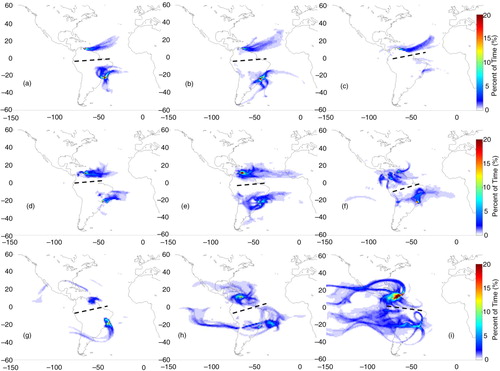
Fig. 5 Origin of air mass based on FLEXPART 14-d back trajectories for cases whose flight layers presented ozone mixing ratios above 40 ppbv over Caracas, Rio de Janeiro or São Paulo in JJA. Colours represent the percent of residence time (or normalised residence time in percent). The columns correspond to flight layers: low troposphere (below 700 hPa) on the left; medium troposphere (between 650 and 380 hPa) on the middle; and upper troposphere (380–180 hPa) on the right panel, while rows correspond to the layers of air mass origin: low troposphere (below 700 hPa) at the top; mid-troposphere (700–380 hPa) on the second line; and from higher altitudes (380 to ~60 hPa) at the bottom panels. The black dashed lines separate trajectories for Caracas from the ones for São Paulo or Rio de Janeiro.

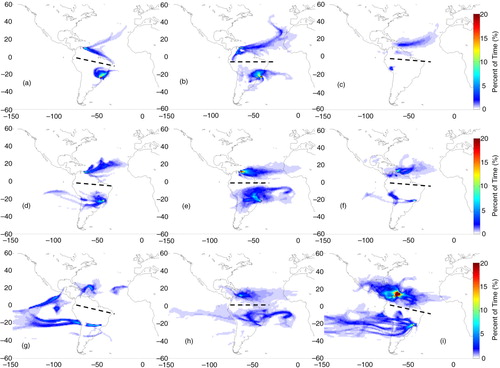
Fig. 6 Origin of air mass based on FLEXPART 14-d back trajectories for cases whose flight layers presented ozone mixing ratios above 40 ppbv over Caracas, Rio de Janeiro or São Paulo in SON. Colours represent the percent of residence time (or normalised residence time in percent). The columns correspond to flight layers: low troposphere (below 700 hPa) on the left; medium troposphere (between 650 and 380 hPa) on the middle; and upper troposphere (380–180 hPa) on the right panel, while rows correspond to the layers of air mass origin: low troposphere (below 700 hPa) at the top; mid-troposphere (700–380 hPa) on the second line; and from higher altitudes (380 to ~60 hPa) at the bottom panels. The black dashed lines separate trajectories for Caracas from the ones for São Paulo or Rio de Janeiro.

Over Caracas, air masses traveling from low levels to the PBL in the four seasons (Figs. 3a, 4a, 5a and 6a) were mostly from local sources. Except for MAM, air masses originated mainly from the northeast (Atlantic) or from the southeast, across the coast. Those are the main directions followed by air masses travelling from low levels, even from northern Africa, with more or less spatial variability depending on the season (first column of Figs. (3–6)).

The second row of Figs. (3–6) shows that except in DJF and SON, air mass origin at intermediate levels prevails from the east, around West Africa. In DJF and SON, the pattern was similar to the observed on the first row. Finally, air masses from the upper layers (third row) were predominantly from the west, with contributions from the Pacific, North and Central America and the Caribbean's in DJF and MAM. Air masses from the south, originating over South America, were observed mainly in MAM. In JJA and SON, contributions from the east were also observed.

In São Paulo and Rio de Janeiro, compared to Caracas, air masses presented higher variability regarding their origin in different seasons and altitudes. In DJF from lower levels, the main direction was from the east (Fig. 3b and c), except in the PBL, where air masses came mostly from the continent, with contributions from the Atlantic Ocean (Fig. 3a). Both in the PBL and the mid-troposphere, the residence time was higher closer to the cities, indicating a significant impact of local sources, a pattern observed in the four seasons (subpanels a and b in Figs. (3–6)). From the intermediate altitudes (second row of Fig. 3), contributions from the continent were also observed, besides the eastern direction, being mainly from southwest in the flight altitude located in the PBL (Fig. 3d) and without a defined path in the upper troposphere (Fig. 3f). From the higher altitudes (third row), air mass origin was predominant from the west, in the Pacific Ocean and following an anti-cyclonic circulation, a pattern observed in the four seasons.

In MAM, the origin of air masses, from lower levels to the PBL, was mainly from the north over land (Fig. 4a). To intermediate levels, air masses originated on the coast, with some contribution from the south, over the Atlantic Ocean (Fig. 4b). Air masses arriving from intermediate levels (second row in Fig. 4) had a northeast component towards the PBL as shown in Fig. 4d; anti-cyclonic circulation both from the continent and the Atlantic Ocean contributed to the enhanced concentrations in the mid-troposphere (Fig. 4e); and originated mainly from the north to the upper troposphere (Fig. 4f). The main difference in JJA and SON is that polluted air masses were mostly from the west, with minor contributions from the Atlantic Ocean.

3.3. Seasonal variability of the geographical distribution of biomass burning fires and lightning in the American and African continents

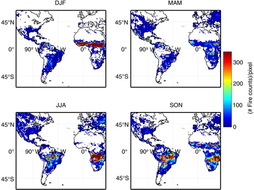
According to MODIS fire count seasonal climatology maps presented in Fig. 7, fire pixels could be observed throughout the year in both continents with large seasonal variability, as a consequence of the Intertropical Convergence Zone annual shift. In DJF, the largest numbers of fire pixels were detected in the Northern Hemisphere. In the African continent, biomass burning activities were detected south of the Sahara desert in a vast west-to-east band, extending from about 5°N to 15°N. In South America, they were concentrated over Venezuela. In MAM, fire counts peaked in Venezuela, Central America and in a small area in Central Brazil, whereas they decreased over Africa. Peaks moved further south in both continents in JJA, reaching the Amazonian deforestation arc in Brazil, Bolivia and Paraguay and covering the largest area over Africa, in the Southern Hemisphere, below the equator down to about 15°S. Figure 7 shows that in SON the area covered by fire pixels is largest over South America, particularly over the arc of deforestation in Brazil, Bolivia, Paraguay and north of Argentina. In Africa, fires were still detected in the central part of the continent and restarted in the northern portion, in the same corridor observed in DJF.

Fig. 7 Mean seasonal number of fire counts per pixel based on MODIS (Moderate Resolution Imaging Spectroradiometer) on board Terra satellite monthly data in the area delimited by latitude from −60° to 60° and longitude from −120° to 40°. Data from January 2002 to December 2012 (available at www.mirador.gsfc.nasa.gov/, – last accessed on 20 February 2014).

The LIS flash rates (Fig. 8) show that seasonal variability was more important in North and Central Americas. In DJF, the highest rates were observed in Central Africa (around the equator), and in its eastern portion, around 25°S; and from the northeast of Brazil down to Argentina, where the maximum was observed in South America. In the same season, minimum flash rates were detected in Central and North America as well as in Venezuela, coinciding with the analysis presented by Collier et al. (2013) who addressed minimum lightning frequency over Venezuela from mid-December to March and maximum from August to October. They analysed lightning data from the Optical Transient Detector and satellite instruments over different countries in South America.

Fig. 8 Mean seasonal climatology of flash rates [# flashes/(km² month)] from LIS (Lightning Imaging Sensor) on board Tropical Rainfall Measuring Mission (TRMM) satellite in the area delimited by latitude from −60° to 60° and longitude from −120° to 40°. Data from 1 January 2008 to 31 December 2012 (available at www.thunder.nsstc.nasa.gov/, last accessed on 12 November 2014).

In MAM, high flash rates persisted over Africa, moving further north and diminished in the south. In America, flash rates decreased below the equator in South America, increased in Central and North America and peaked over Colombia and Venezuela. While flash rate distribution was quite similar to the previous season in Africa, moving a little to the north and east (with a peak over Ethiopia), the number of flash rates increased in Central and North America in JJA, presenting maximum rates around Florida, in the United States, western Mexico and over Colombia and minimum over Brazil. In SON, the lightning frequency decreased in Central and North America and peaked over Colombia and Venezuela, in the south of the Amazon Basin and south of Brazil. In this season, flash rates continued high in Central Africa, peaking over the Democratic Republic of the Congo, in the interior, and over Liberia, in the west coast. Probably due to the Sahara desert, no lightning was observed above 15°N in the African continent. Also, the maximum flash rates over Venezuela were detected in SON, while around São Paulo and Rio de Janeiro, the maximum occurred in DJF with a second peak in SON.

According to Collier et al. (2013), in Brazil, maximum lightning frequency was around October to December and minimum from May to July. Rickenbach et al. (2011), analysing mesoscale convective systems structures in four distinct regions of South America, included 10 yr of lightning flash rates also from TRMM (1998–2007), with results similar to that discussed here. Their region I covered the central and western portions of the Amazon basin, and region II was located to the north–northeast of Brazil. Region III was located north of São Paulo and Rio de Janeiro states, encompassing the northeast portion of São Paulo state and region IV was located to the southwest, covering the western portion of São Paulo state. In region I, lightning flash rates presented a maximum in August–September and minimum from December to about May. Region II presented a broader and weaker maximum around mid-August to November. In region III, the maximum lightning flash rates were observed between August and October and the minimum around June and July. Finally, in region IV, lightning flash rates presented more variability compared to the other regions, with a peak more than twice as high in mid-September, but with several other lower local maxima from July to October and also around March–April. According to the authors, the noisier behaviour was due to the influence of wintertime baroclinic systems and the lack of a strong annual cycle, while the highest peak in lightning flash rates was due to the predominance of mesoscale convective complexes in the region.

3.4. Analysis of CO and O₃ distribution maps from IASI

As already mentioned, in the boundary layer, one of the pressure levels with independent information for carbon monoxide from IASI retrievals is around 800 hPa. In Fig. 9, seasonal maps are presented for CO at this pressure level. A persistent plume over Africa and the western portion of the tropical Atlantic Ocean, south of about 5°S is observed all year round. In DJF, the high concentrations located between the Equator and 10°N from Western to Eastern Africa are coincident with the highest fire counts. The high CO concentrations detected over central Africa and the gulf of Guinea result from the strong Harmattan wind blowing from northeast Africa and transporting CO from the BB region (Fig. 10, DJF). In SON, the plume is shifted to the south, coincident with the fire count seasonal maps of Fig. 7.

Fig. 9 Seasonal maps of carbon monoxide mixing ratio in ppbv at 800 hPa retrieved from IASI measurements on board MetOp-A satellite: (a) DJF; (b) MAM; (c) JJA; and (d) SON based on data from years 2008 to 2012.

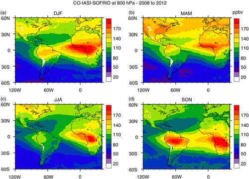
Fig. 10 Horizontal wind vector (m s⁻¹) seasonal maps at 800 hPa from ECMWF ERA-Interim Global Reanalysis at 0.25°×0.25° resolution based on 2008–2012 data.

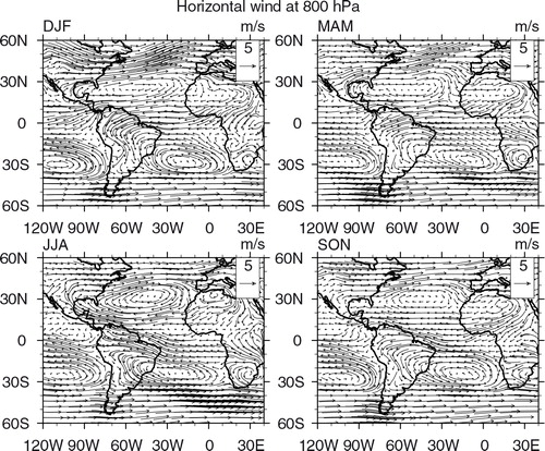
In South America, the highest concentrations of CO around Colombia and Venezuela are observed in MAM and in SON over central Brazil. Returning to the fire pixel count maps from Fig. 7, we conclude that biomass burning is also the source of the enhanced concentrations in those regions. In DJF, this second maximum is located between 0° and 15°S, possibly due to vegetation fires from the northern part of the continent or from long-range transport from Africa (see the wind map in Fig. 10). Over Central and North America, the highest mixing ratios are observed in MAM, especially in the southeast and western portions of the United States. In this region, anthropogenic emissions are the dominant CO source. It is interesting to note that although in JJA, fire counts are high in the central part of South America, the peak of the CO plume is located further west, through transport towards the Pacific Ocean by the strong easterly winds (Fig. 10), and uplifted to higher altitudes across the Andes mountains as shown in Fig. 11.

Fig. 11 Seasonal maps of carbon monoxide mixing ratio in ppbv at 220 hPa retrieved from IASI measurements on board MetOp-A satellite: (a) DJF; (b) MAM; (c) JJA; (d) SON based on data from years 2008 to 2012.

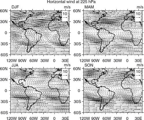
High CO concentrations measured in the upper troposphere in SON over São Paulo and Rio de Janeiro (Fig. 2) were due to local anthropogenic sources or South American vegetation fires without contribution from Africa, as pointed before. The CO maps at 220 hPa in Fig. 11 and horizontal wind maps at 500 and 225 hPa, respectively, in Figs. 12 and 13 corroborate this analysis. In SON, a high altitude anticyclone is centred over southwestern Brazil, and westerly winds prevail in the mid and upper troposphere, south of about 15°S, inhibiting air masses from Africa being transported to South America. Furthermore, our back trajectory analysis gives no indication of transport from Africa or the Atlantic Ocean in SON towards São Paulo and Rio de Janeiro either (Fig. 6).

Fig. 12 Horizontal wind vector (m s⁻¹) seasonal maps at 500 hPa from ECMWF ERA-Interim Global Reanalysis at 0.25°×0.25° resolution based on 2008–2012 data.

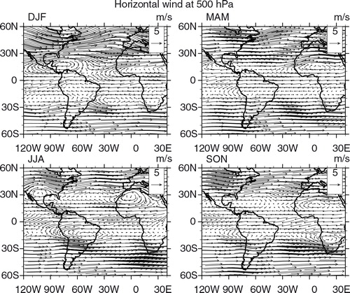
Fig. 13 Horizontal wind vector (m s⁻¹) seasonal maps at 225 hPa from ECMWF ERA-Interim Global Reanalysis at 0.25°×0.25° resolution based on 2008–2012 data.

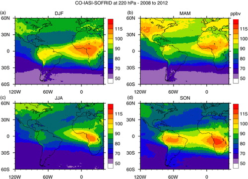
Distribution maps of ozone from IASI retrievals at 520 and 220 hPa are presented in Figs. 14 and 15, respectively. Starting with the 520 hPa level, the O₃ high concentrations detected over northern Africa and especially over the Saharan desert are erroneous because they result from surface emissivity problems. A persistent plume is observed over the Atlantic Ocean, close to the Brazilian northeast coast, south of the equator and can be associated with the zonal wave-one pattern (Thompson et al., 2000; Edwards et al., 2003; Jenkins and Ryu, 2004; Sauvage et al., 2006). From the horizontal wind and lightning maps (Figs. 12 and 8, respectively), the origin of that ozone in the mid-troposphere includes lightning from Africa, as suggested by Sauvage et al. (2006). Lightning from the northeast portion of South America in DJF is also a possible source (Fig. 8; Jenkins and Ryu, 2004). In JJA, precursors from biomass burning in South America can also be transported by the anti-cyclonic circulation centred near 10–20°S, although the location of the ozone plume in this season contrasts with the one for CO, located further west. One possible explanation is that lightning from the south contributed to this plume, transported by the anti-cyclonic circulation at 500 hPa, while biomass burning products were transported to the northwest in the PBL being lifted up by convection further away from the sources. Finally, both lightning and biomass burning from South America, as well as fires from southern Africa and lightning from Central Africa in SON, could have contributed to this plume as pointed out by Sauvage et al. (2006). São Paulo and Rio de Janeiro are located south of this plume and, depending on the season, might also be contaminated by it due to the presence of the anti-cyclonic circulation.

Fig. 14 Seasonal maps of ozone mixing ratio in ppbv at 520 hPa retrieved from IASI measurements on board MetOp-A satellite: (a) DJF; (b) MAM; (c) JJA; (d) SON based on data from years 2008 to 2012.

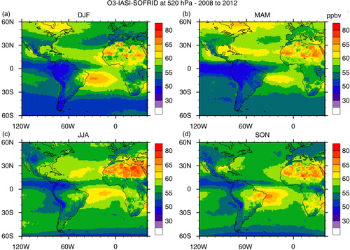
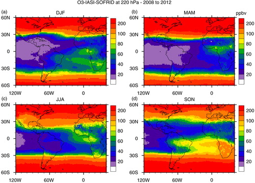
Fig. 15 Seasonal maps of ozone mixing ratio in ppbv at 220 hPa retrieved from IASI measurements on board MetOp-A satellite: (a) DJF; (b) MAM; (c) JJA; (d) SON based on data from years 2008 to 2012.

In DJF, an anti-cyclonic circulation is observed over Central America. Transport from Central and North Americas to the northernmost South America, around Venezuela could be responsible for the ozone mixing ratio at 520 hPa, where no local plume is evidenced in the O₃ map. In MAM, transport of biomass burning precursors from Central America and West Africa and anthropogenic emissions and lightning from North America and Central Africa are possible sources of the plume located over the Tropical North Atlantic and the Caribbean's. Wind from the west is observed at northern latitudes and from the east further south in this season (Fig. 12), indicating that this plume could also reach Caracas. In JJA, the wind map indicates that air masses in Venezuela are from Africa, confirmed by back trajectories (Fig. 5). In SON, contributions from both the Caribbean and Africa could be expected, although the back trajectories indicate that the Caribbean contributes only if there are downdrafts from the upper atmosphere (Fig. 6h).

In MAM and JJA, the ozone plume at 220 hPa is limited to Africa and the Gulf of Guinea (Fig. 15). Note also that as discussed previously, the lightning frequency is low in JJA. Despite the fact that fire counts were high in South America in this season, no ozone enhancement is observed indicating that there is no vertical transport of ozone or its precursors to the upper troposphere due to the lack of deep convection. In contrast, in DJF and SON, the ozone plume extends over south tropical Atlantic and the western part of South America. Observations from IASI clearly indicate SON as the season of the annual maximum for this upper tropospheric O₃ plume as already observed by other satellite instruments such as Total Ozone Mapping Spectrometer (TOMS) and Solar Backscattered Ultra Violet (SBUV) (Fishman et al., 1990, 2003). This seasonal maximum results from a combination of lightning and biomass burning sources from both continents as discussed in Sauvage et al. (2007a). As already discussed for CO, São Paulo and Rio de Janeiro are located further south where strong westerly winds prevail (Fig. 13), and the possible sources of ozone over these cities are therefore lightning and biomass burning from South America.

3.5. Integration of GEOS-Chem model results with previous analyses

In this section, results from the sensitivity tests performed with GEOS-Chem CTM are discussed. Starting with the results over Caracas for the year 2007 and for CO simulations, GEOS-Chem in general reproduced higher altitude mean concentrations within 1 SD (Fig. 16). MAM was the exception, when numerical simulations underestimated the observed mean concentrations at all altitudes. In the PBL, the model underestimated the high CO concentrations in all the seasons, indicating its inability to capture local anthropogenic emissions. Particularly in MAM, Fig. 9 illustrates elevated CO concentration at 800 hPa over Venezuela. From Figs. 9 and 7, local biomass burning and from Central America could also be an important source to the observed pollution. Still from Fig. 9 and wind map from Fig. 10, anthropogenic emissions from North America could also present some contributions. One reason for the observed underestimation could be the biomass burning inventory. For instance, Longo et al. (2010) proposed a new technique to estimate biomass burning emissions of trace gases over South America, based on remote sensing fire products and field observations. They compared the results of the new technique with several available inventories, including GFED2, the same as used in the present analysis and concluded that GFED2 systematically underestimated CO concentrations. Most available inventories of biomass burning emission are based on fire counts retrieved from satellite data. Limitations intrinsic to the technique are attributed, for instance, to sensor channel saturation by high temperatures, undetected or missed fires, cloud cover that can mask the detection of fires under the cloud fields, all causing underestimation of the emissions (Pereira et al., 2009). In fact, other studies reported that GFED2 inventory might underestimate CO emissions (van der Werf et al., 2006; Jones et al., 2009; Turquety et al., 2009; Barret et al., 2010). Recent versions of the model from v-01-02 and later accept GFED3 updated inventory, which might have solved this issue. Another reason for the model failure to capture PBL CO higher concentrations is that local anthropogenic emission source could also have been underestimated for Caracas, a problem common to global models due to the low horizontal resolution. Moreover, Alonso et al. (2010) compared their local inventories based on mobile sources for anthropogenic emissions with EDGAR using a regional atmospheric chemistry model for some cities in South America. There is no result for Caracas but for Bogotá, in Colômbia, EDGAR annual emission rate for CO was underestimated by 23.5%, while for NO _x it was overestimated by 37% when compared with their inventories. According to the authors, the difference over São Paulo for NO _x can vary by a factor of 2, indicating a potential problem with EDGAR inventory over South America for anthropogenic emission. Also, Caracas is located on the coast and land/ocean mask for the emission inventory could cause dilution of pollutants in the region. Finally, the location of Caracas on the coast, next to high hills, favours the accumulation of pollution, not captured by models with coarse horizontal resolution.

Fig. 16 Comparison of seasonal mean vertical profile of carbon monoxide concentrations measured over Caracas and estimated numerically with GEOS-Chem for the year 2007. Grey shading represents the SD of the measured concentrations and indicates their variability throughout the season.

Figure 17 presents the mean seasonal profiles of O₃ concentrations from measurements and from GEOS-Chem run outputs. In the four seasons, anthropogenic local emissions are the main ozone precursor source close to the surface, with detectable influence up to the upper troposphere. During DJF, GEOS-Chem runs systematically overestimated the measured concentrations above ~750 hPa. The second important precursor source is lightning from South America followed by lightning from Africa. Lightning from South America becomes the most important source in the upper troposphere. No influence from biomass burning coming from Africa was detected by the model which attributed about 5 ppbv at high altitudes to biomass burning from South America in this season. According to Section 3.3 and Collier et al. (2013), the DJF season is expected to present minimum lightning activity in Venezuela. However, from the lightning flash rate (Fig. 8) and 225 hPa wind maps (Fig. 13), lightning from the northeast of Brazil, where precursors were transported by the anti-cyclonic circulation, could have been captured by the model. Moreover, from the satellite fire counts (Fig. 7) and 500 hPa wind maps (Fig. 12), biomass burning either from local sources in Venezuela and Colombia or from Central America, which re-circulated over the Caribbean could also have contributed. The map of carbon monoxide seasonal mean concentration at 800 hPa for DJF presented in Fig. 9 shows that CO transport over the Atlantic Ocean coming from Africa was further south, at least in the PBL. In contrast, the maps for ozone and wind at 520 hPa in Figs. 14 and 12, respectively, indicate that some contribution from lightning coming from Central Africa and North America could also be possible. Back trajectories from Fig. 3 indicate that ozone from northern African continent could also be transported towards Caracas, due to lightning as described by Edwards et al. (2003).

Fig. 17 Comparison of seasonal mean vertical profile of ozone concentrations measured over Caracas and estimated numerically with GEOS-Chem for year 2007. Five different runs were performed, considering all NO _x emission sources and turning off NO _x emissions from biomass burning and lightning from Africa and South America in sensitivity analysis tests. Grey shading represents the SD of the measured concentrations and indicates their variability throughout the season.

During MAM, the mean seasonal concentration of ozone from the model was inside 1 SD from the measured mean, above 700 hPa. In the PBL, GEOS-Chem underestimated ozone concentration by more than 30 ppbv around 800 hPa, indicating a potential problem in representing photochemical processes from biomass burning or urban emissions. Again, anthropogenic sources followed by lightning from South America were identified as the main precursor sources of ozone, the latter in the mid and upper troposphere. From the higher altitude wind maps at 500 and 225 hPa, combined with the flash rates map, the possible source origin could be lightning from Colombia and Venezuela, with some contributions also from Central and North America. Back trajectories in Fig. 4f, h and i corroborate this result. Biomass burning contribution either from South America or Africa was negligible in the model, although fires in Venezuela were common in this period of the year, as shown in Fig. 7 and confirmed by CO concentration map presented in Fig. 9, which could explain why the model could not capture the peak in the PBL. As for CO, biomass burning from Central America and anthropogenic emissions from North America could also impact the observed ozone peak.

In JJA, GEOS-Chem represented the mean ozone profile within 1 SD and attributed lightning from Africa as a significant source of precursors, followed by anthropogenic emissions and biomass burning from South America, where fires are more common to the south of the Amazon basin and Maranhão state (Fig. 7). Also, lightning from South America affected the ozone profile in the upper layers. From the 800 hPa wind map (Fig. 10), fire products from Maranhão could be transported towards Caracas. Wind maps for higher levels (Figs. 12 and 13), combined with flash rates from Fig. 8, indicate that lightning from Colombia, the Caribbean, Central and North America as well as from northern Africa could also have contributed to the enhancement of ozone concentration in this season, as well as anthropogenic emission from the southernmost North America. Maps of CO and O₃ concentrations presented in Figs. 9 and 14, respectively, corroborate lightning from Africa as the main source of ozone precursors, given that no carbon monoxide from Africa was transported to Caracas region, while one can observe the ozone plume crossing the Atlantic Ocean in a corridor north of the equator. Back trajectories also corroborate those findings (Fig. 5). However, the model could not represent the peak concentrations in the mid and upper troposphere. Sauvage et al. (2007b) attributed the problem to the convective parameterisation based on the Relaxed Arakawa Schubert, which tends to overestimate ozone concentration at high levels. According to Mitovski et al. (2012), it is difficult to assess the accuracy of convective transport in a global model. The difficulty comes from the fact that in global chemical transport models, the spatial scale of convective clouds is much smaller than the grid scale, so that the convective transport of chemical tracers is parameterised rather than explicitly modelled.

In SON, GEOS-Chem systematically underestimated the observed concentration, in particular above 600 hPa. After anthropogenic emissions, lightning from Africa was identified to cause the higher variability in the ozone profile mainly in low and intermediate levels and from South America at higher altitudes. No influence from biomass burning emissions was identified. From the PBL and upper troposphere wind (Figs. 10 and 13, respectively), fire counts (Fig. 7) and flash rates maps (Fig. 8), both biomass burning from the northeast of Brazil (at lower altitudes) and lightning from the Amazon (at higher altitudes) could have contributed to the observed concentrations. At intermediate altitudes, ozone produced by lightning from Africa and Central America, in this case, transported by the anti-cyclonic circulation centred over the Caribbean Sea, could also reach Caracas (Fig. 12). The ozone seasonal mean concentration map from Fig. 14 confirms that contribution from Central and North Americas and the Caribbean was also possible. Back trajectories in Fig. 6 corroborate the transport from the coast of Brazil from low and intermediate levels (Fig. 6a–e) and from Africa and the Caribbean from intermediate and upper levels (Fig. 6f, h and i). Again, the model failed to capture the mid and upper troposphere peak. According to Torres et al. (2010), the year 2007 was characterised by a severe dry season in South America, and the number of detected fires from satellite was the largest from the 10 years analysed period (2000–2009) in their study. Thus, comparing ozone mean climatological profile in Fig. 1 for JJA and SON with the year 2007 for the same seasons, the mid-troposphere peak observed in both seasons in 2007 might have been produced by fires from Brazil, underestimated by the model. Also, the convective parameterisation problem discussed previously can have moved these peaks too high.

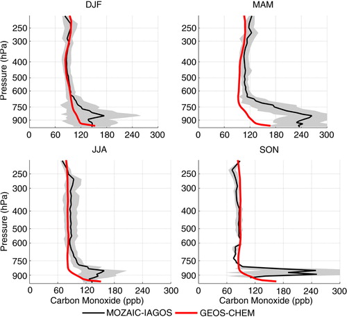
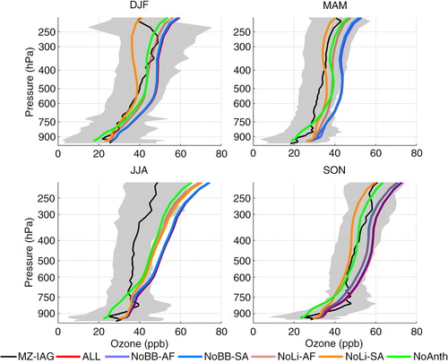
Comparison of the GEOS-Chem simulations for CO concentrations with observations over São Paulo and Rio de Janeiro, presented in Fig. 18, shows that the model captured the main sources below 600 hPa, representing the mean concentration within 1 SD from the observations in all the seasons, except in SON, when the model underestimated the mean concentrations. According to Freitas et al. (2005), the main corridor of smoke export to the Atlantic Ocean is further south, reaching mainly the southernmost portion of Brazil, north of Argentina and Uruguay. This corridor is due to the barrier caused by the Andes on the western side and an anti-cyclonic circulation over the Atlantic Ocean. This pattern is changed only when some atmospheric perturbations take place, such as a cold front system, depleting the plume to the east, allowing the transport of the smoke plume over São Paulo and Rio de Janeiro. Thus, the lack of this contribution from GEOS-Chem results could be due to the fact that no systems transported the plume towards southeast Brazil in 2009, when compared with the measurements performed in earlier years. Figure 9 for SON, however, indicates that this was not the case since it shows that the CO plume encompasses the whole of the northern portion of South America down to about 25°S, remembering that the map was built using data from 2009 also. As mentioned before, CO and wind maps [225] at 220 hPa (Figs. 11 and 13) show that the peak from biomass burning origin observed above 400 hPa is also underestimated by the model, again indicating a problem with GFED2. However, the good representation of PBL CO, during the other seasons, indicates that local anthropogenic emissions are well represented by GEOS-Chem in this region.

Fig. 18 Comparison of climatological seasonal mean vertical profile of carbon monoxide concentrations measured over Rio de Janeiro and São Paulo and estimated numerically with GEOS-Chem for the representative year 2009. Grey shading represents the SD of the measured concentrations and indicates their variability throughout the season.

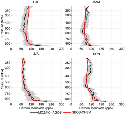
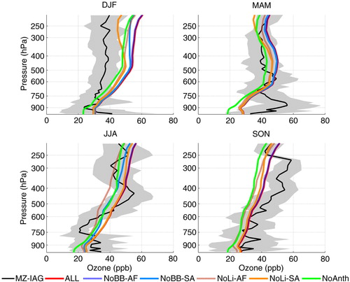
Figure 19 presents the seasonal mean of ozone profiles based on the entire database measured over Rio de Janeiro and São Paulo compared to GEOS-Chem runs performed for the year 2009 when the control runs (including all the possible emission sources in the model) better represented the observed means, as already mentioned. GEOS-Chem represented the observed concentrations within 1 SD in DJF and SON, but systematically overestimated the observed means in the other two seasons. In MAM, numerical results were in the upper limit of 1 SD in all altitudes, while in JJA, below about 550 hPa, GEOS-Chem results were within 1 SD but overestimated aloft. Except for this season, the main source of NO _x able to cause the highest variability on the ozone concentration was lightning from South America (from 10 to ~15 ppbv), followed by anthropogenic local emissions and lightning from Africa (~3–5 ppbv). This result agrees with the seasonal variability for lightning over South America, which presented minimum flash rates in JJA, maximum activity in DJF and a second peak in SON, as shown in Fig. 8.

Fig. 19 Comparison of climatological seasonal mean vertical profile of ozone concentrations measured over Rio de Janeiro and São Paulo and estimated numerically with GEOS-Chem for year 2009. Five different runs were performed, considering all NO _x emission sources and turning off NO _x emissions from biomass burning and lightning from Africa and South America in sensitivity analysis tests. Grey shading represents the SD of the measured concentrations and indicates their variability throughout the season.

In DJF and MAM, at 500 hPa, the maps presented in Fig. 12 illustrate that the wind prevails from the west at latitudes below 20°S, transporting NO _x produced by lightning, located mainly to the southwest and west (Fig. 8). Back trajectories, from Figs. 3h, for DJF, and 4f, for MAM, show that the air masses were transported to the cities from the upper troposphere. Moreover, in both seasons, the anti-cyclonic circulation can also import ozone from the region of the Tropical Atlantic paradox, where high ozone concentration is frequently observed; back trajectories corroborate this for low and mid troposphere (Figs. 3b, d, e and 4b, d–f). In contrast, ozone peaks in central Brazil, coincident with the largest fire counts region in JJA (Fig. 7), although as discussed previously, CO maps indicate that fire products from this source were mainly transported to the northwest. The latter explains the small contribution from this source attributed by the model around 750 hPa. GEOS-Chem assigned anthropogenic emissions and lightning from Africa and South America as the ozone precursor sources in this season. Wind maps at 500 hPa (Fig. 12) indicate that transport from the ozone plume located over central Brazil and the Atlantic Ocean is plausible. In previous discussion about the ozone plume, lightning from the south of Brazil can be a potential source to its formation, as well as from Africa. Back trajectories from polluted cases presented in Fig. 5 suggest origin over the continent from low and intermediate altitudes and even from the Pacific from upper layers.

In SON, GEOS-Chem identified lightning from South America as the main ozone precursor source, followed by anthropogenic emissions and then biomass burning also from South America and lightning from Africa. According to the wind maps, only at 500 hPa (Fig. 12) ozone could be transported from the Tropical Atlantic towards São Paulo and Rio de Janeiro and only after recirculating over the continent. However, as discussed in the previous section, this Tropical Atlantic plume is due to a combination of fire and lightning from both continents. From the upper troposphere wind map presented in Fig. 13, only the westerly wind from the Pacific and recirculation from the continent prevail towards São Paulo and Rio de Janeiro. The 14-d back trajectory climatology for this region, presented on the second and third rows of Fig. 6, corroborates this behaviour. Thus, the results indicate that the model could capture the influence of South American lightning to ozone production but overestimating the concentration and performed poorly in representing the contribution of biomass burning from South America. Moreover, if lightning from Africa had contributed to the observed ozone in this season, contribution from African fires should have been detected too, noting that there is also a CO plume over the Atlantic Ocean.

In all the seasons, the modelled concentration of O₃ showed a rapid increase with altitude above ~300 hPa, particularly in JJA, even though this season presented the less sensitivity to the perturbed sources and less lightning, indicating less convective activity. For the other seasons as discussed previously over Caracas, the convective parameterisation might be the source of the overestimation, remembering that in those seasons lightning from South America was identified as the main source of ozone precursors by the model. For JJA, since it is the season with the higher frequency of occurrence of STE events over São Paulo, caused by the subtropical and polar jets (Yamasoe et al., 2015), this analysis should be explored in the future to verify if this effect is overestimated by GEOS-Chem.

4. Conclusions

This study analysed vertical profiles of ozone and carbon monoxide measured during landing and take-off of commercial aircrafts as part of the MOZAIC and IAGOS programmes at Caracas, Rio de Janeiro and São Paulo. Even though the frequency of flights in this part of the world was rather irregular, MOZAIC/IAGOS databases were useful to explore the seasonal variability of both ozone and carbon monoxide in the troposphere. The model strengthened the importance of anthropogenic local emissions over the three analysed cities particularly in the PBL. In terms of seasonal variability, the season with elevated ozone and CO concentrations coincided with the peak of the biomass burning season in both regions. Over Caracas, the maximum concentrations were observed in March to May, while in São Paulo and Rio de Janeiro the maximum was observed from September to November.

Over Caracas, from the surface up to 200 hPa, MAM presented the highest mean value of POC, with more than 24 DU, while December to February presented the lowest, varying from 15 DU in 1997 to 22 DU 2007, indicating relatively clean conditions. Considering interannual variability, no trend was observed in the tropospheric ozone mixing ratio.

Over São Paulo and Rio de Janeiro, the highest ozone concentration was observed during SON, with mean POC, integrated from the surface up to 200 hPa, reaching about 30 DU in 2012. Although no trend analysis could be performed due to the rather irregular frequency of flights over this area, results indicated a possible tendency of increasing concentrations in the recent years at 95% significance level.

From the back trajectories analysis using FLEXPART model, the main corridors of pollutants transport towards Caracas were from the northeast, over the Atlantic Ocean and as far as from Africa and from the southeast boarding the coast. Central and North Americas as well as the Caribbean were also identified as potential sources, mainly from higher altitudes. Eastern origin was observed from intermediate and higher altitudes. Over São Paulo and Rio de Janeiro, results presented larger variability, with contributions from the continent and both from the Atlantic and Pacific Oceans. Air masses from the Atlantic were transported mainly at lower and intermediate levels and in DJF and MAM. In JJA and SON, air masses were predominantly from the continent. From upper layers, western origin prevailed in all seasons, as far as the Pacific.

Satellite products as fire counts from MODIS, lightning flash rates from LIS and O₃ and CO from IASI as well as wind maps from different pressure levels helped interpreting GEOS-Chem sensitivity analysis on the identification of contributions from biomass burning and lightning from South American and African continents as well as other source regions, particularly over Caracas. From those maps, Central and North Americas and the Caribbean also export pollution towards Caracas, either from anthropogenic emissions in the case of North America or from lightning and biomass burning activities.

Sensitivity analyses performed with GEOS-Chem showed that lightning produced in South America is an important source of ozone precursors over São Paulo and Rio de Janeiro, except in JJA the only season when anthropogenic emissions were more important even above the PBL. The model captured the seasonal variability of the lightning activity, although improvements are still needed since modelling results appear to overestimate measurements and did not capture the observed influence of biomass burning from South America. Results for CO corroborates this finding, since GEOS-Chem, in general, reproduced CO mean concentration even below 600 hPa, except in SON, when biomass burning is the major source over the region. The observed good performance in the other seasons indicates that the model could capture the influence of the local anthropogenic emission in the region. In contrast, in SON, the model systematically underestimated the observed mean concentration. The same result was obtained over Caracas in MAM, also the season with the largest number of fire counts in the region. No influence of biomass burning from Africa was detected by the model.

Over Caracas, the model could capture the influence of lightning long-range transported from Africa as an important ozone precursor source in JJA and SON, corroborated by the back trajectories analysis and satellite maps. Although lightning activity is minimum in the Venezuelan region in DJF, the model attributed lightning from South America as an important source. From the satellite data and wind maps, we conclude that the model was able to capture the influence of lightning from the northeast of Brazil.

The synergy between in situ measurements, satellite retrievals and modelling studies helped us to have a better knowledge on the carbon monoxide and ozone precursor sources over South America, outside the Amazon Basin, where most of the studies were performed in the recent decades. As expected, anthropogenic local emissions had a significant impact in perturbing the ozone profile and the GEOS-Chem model performed well in capturing their influence, particularly for CO over São Paulo and Rio de Janeiro. Biomass burning contributions is believed to be underestimated in our study, but this potential problem might have been solved in more recent versions of GEOS-Chem since they allow the use of GFED3 with more up-to-date information. The analysis showed the significant impact of lightning from South America and to a lesser extent from Africa on the ozone formation. The model could even reproduce the seasonal variability of lightning over South America. The anthropogenic emission inventory particularly over smaller cities as Caracas was underestimated in the model. The convective parameterisation and STE, on the other hand, overestimated ozone concentration in the mid and upper troposphere. Revision on these items will help improve the performance of the model over South America in future studies.

Acknowledgements

The authors acknowledge the support of the European Commission to the MOZAIC project (1994–2003) and the preparatory phase of IAGOS (2005–2012), Airbus and the Airlines (Lufthansa, Air-France, Austrian, Air Namibia, Cathay Pacific and China Airlines so far) for carrying the MOZAIC or IAGOS equipment and for performing the maintenance since 1994. MOZAIC is presently funded by INSU-CNRS (France), Météo-France, CNES, Université Paul Sabatier (Toulouse, France) and Research Center Jülich (FZJ, Jülich, Germany). The MOZAIC-IAGOS data are available at www.pole-ether.fr, thanks to the support from ETHER, French data centre service. M.A. Yamasoe thanks Conselho Nacional de Desenvolvimento Científico e Tecnológico (CNPq) and Ciências sem Fronteira Program for grant number 237032/2012-0, and Coordenação de Aperfeiçoamento de Pessoal de Nível Superior (CAPES). She also acknowledges all the staff from the Laboratoire d'Aérologie for the help during her visit. The Lightning Imaging Sensor (LIS) Science Data were obtained from the NASA EOSDIS Global Hydrology Resource Center (GHRC) DAAC, Huntsville, AL, www.thunder.nsstc.nasa.gov/. Fire counts from MODIS (Moderate Resolution Imaging Spectroradiometer) on board Terra satellite were obtained using Mirador Earth Science Data Search Tool, www.mirador.gsfc.nasa.gov/. Thanks to the European Centre for Medium-Range Weather Forecasts (ECMWF) for making available the Global Reanalysis ERA Interim data at www.apps.ecmwf.int/datasets/data/interim_full_moda/. Finally, we acknowledge the anonymous referees for their time and thorough review of the manuscript and their constructive suggestions.

Notes

This paper is part of a Special Issue on MOZAIC-IAGOS in Tellus B celebrating 20 years of an ongoing air chemistry climate research measurements from airbus commerical aircraft operated by an international consortium of countries. More papers from this issue can be found at http://www.tellusb.net

References

- Alonso M. F. , Longo K. M. , Freitas S. R. , Fonseca R. M. , Marécal V. , co-authors . An urban emissions inventory for South America and its application in numerical modeling of atmospheric chemical composition at local and regional scales. Atmos. Environ. 2010; 44: 5072–5083.
- Andrade M. F. , Fornaro A. , Freitas E. D. , Mazzoli C. R. , Martins L. D. , co-authors . Ozone sounding in the Metropolitan Area of São Paulo, Brazil: wet and dry season campaigns of 2006. Atmos. Environ. 2012; 61: 627–640.
- Andreae M. O. , Artaxo P. , Beck V. , Bela M. , Freitas S. , co-authors . Carbon monoxide and related trace gases and aerosols over the Amazon Basin during the wet and dry seasons. Atmos. Chem. Phys. 2012; 12: 6041–6065. DOI: http://dx.doi.org/10.5194/acp-12-6041-2012 .
- Andreae M. O. , Merlet P . Emission of trace gases and aerosols from biomass burning. Global Biogeochem. Cycles. 2001; 15(4): 955–966.
- Ashmore M. R . Assessing the future global impacts of ozone on vegetation. Plant Cell Environ. 2005; 28: 949–964.
- Barret B. , Le Flochmoen E. , Sauvage B. , Pavelin E. , Matricardi M. , co-authors . The detection of post-monsoon tropospheric ozone variability over south Asia using IASI data. Atmos. Chem. Phys. 2011; 11: 9533–9548. DOI: http://dx.doi.org/10.5194/acp-11-9533-2011 .
- Barret B. , Williams J. E. , Bouarar I. , Yang X. , Josse B. , co-authors . Impact of West African Monsoon convective transport and lightning NOx production upon the upper tropospheric composition: a multi-model study. Atmos. Chem. Phys. 2010; 10: 5719–5738.
- Bey I. , Jacob D. J. , Yantosca R. M. , Logan J. A. , Field B. D. , co-authors . Global modeling of tropospheric chemistry with assimilated meteorology: model description and evaluation. J. Geophys. Res. 2001; 106(D19): 23073–23095.
- Collier A. B. , Bürgesser R. E. , Ávila E. E . Suitable regions for assessing long term trends in lightning activity. J. Atmos. Sol. Terr. Phys. 2013; 92: 100–104.
- Curtis L. , Rea W. , Smith-Willis P. , Fenyves E. , Pan Y . Adverse health effects of outdoor air pollutants. Environ. Int. 2006; 32: 815–830.
- De Wachter E. , Barret B. , Le Flochmoën E. , Pavelin E. , Matricardi M. , co-authors . Retrieval of MetOp-A/IASI CO profiles and validation with MOZAIC data. Atmos. Meas. Tech. 2012; 5: 2843–2857. DOI: http://dx.doi.org/10.5194/amt-5-2843-2012 .
- Dufour G. , Eremenko M. , Griesfeller A. , Barret B. , LeFlochmoën E. , co-authors . Validation of three different scientific ozone products retrieved from IASI spectra using ozonesondes. Atmos. Meas. Tech. 2012; 5: 611–630.
- Duncan B. N. , Logan J. A. , Bey I. , Megretskaia I. A. , Yantosca R. M. , co-authors . Global budget of CO, 1988–1997: source estimates and validation with a global model. J. Geophys. Res. 2007; 112(D22): 22301. DOI: http://dx.doi.org/10.1029/2007JD008459 .
- Edwards D. P. , Lamarque J.-F. , Attié J.-L. , Emmons L. K. , Richter A. , co-authors . Tropospheric ozone over the tropical Atlantic: a satellite perspective. J. Geophys. Res. 2003; 108(D8): 4237. DOI: http://dx.doi.org/10.1029/2002JD002927 .
- Fishman J. , Watson C. E. , Larsen J. C. , Logan J. A . Distribution of tropospheric ozone determined from satellite data. J. Geophys. Res. 1990; 95(D4): 3599–3617.
- Fishman J. , Wozniak A. E. , Creilson J. K . Global distribution of tropospheric ozone from satellite measurements using the empirically corrected tropospheric ozone residual technique: identification of the regional aspects of air pollution. Atmos. Chem. Phys. 2003; 3: 893–907.
- Freitas S. R. , Longo K. M. , Dias M. A. F. S. , Dias P. L. S. , Chatfield R. , co-authors . Monitoring the transport of biomass burning emissions in South America. Environ. Fluid Mech. 2005; 5: 135–167.
- Galanter M. , Levy H., II. , Carmichael G. R . Impacts of biomass burning on tropospheric CO, NOx, and O3 . J. Geophys. Res. 2000; 105(D5): 6633–6653.
- George M. , Clerbaux C. , Hurtmans D. , Turquety S. , Coheur P.-F. , co-authors . Carbon monoxide distributions from the IASI/METOP mission: evaluation with other space-borne remote sensors. Atmos. Chem. Phys. 2009; 9: 8317–8330.
- Guenther A. , Hewitt C. N. , Erickson D. , Fall R . A global model of natural volatile organic compound emissions. J. Geophys. Res. 1995; 100(D5): 8873–8892.
- Holloway T. , Levy H., II. , Kasibhatla P . Global distribution of carbon monoxide. J. Geophys. Res. 2000; 105(D10): 12123–12147.
- Homeyer C. R. , Bowman K. P . Rossby wave breaking and transport between the tropics and extratropics above the subtropical jet. J. Atmos. Sci. 2013; 70: 607–626. DOI: http://dx.doi.org/10.1175/JAS-D-12-0198.1 .
- Huntrieser H. , Schlager H. , Roiger A. , Lichtenstern M. , Schumann U. , co-authors . Lightning-produced NOx over Brazil during TROCCINOX: airborne measurements in tropical and subtropical thunderstorms and the importance of mesoscale convective systems. Atmos. Chem. Phys. 2007; 7: 2987–3013.
- Iwabe C. M. N. , Rocha R. P . An event of stratospheric air intrusion and its associated secondary surface cyclogenesis over the South Atlantic Ocean. J. Geophys. Res. 2009; 114: 09101. DOI: http://dx.doi.org/10.1029/2008JD011119 .
- Jacob D. J. , Heikes B. G. , Fan S.-M. , Logan J. A. , Mauzerall D. L. , co-authors . Origin of ozone and NOx in the tropical troposphere: a photochemical analysis of aircraft observations over the South Atlantic basin. J. Geophys. Res. 1996; 101(D19): 24235–24250.
- Jaeglé L. , Steinberger L. , Martin R. V. , Chance K . Global partitioning of NOx sources using satellite observations: relative roles of fossil fuel combustion, biomass burning and soil emissions. Faraday Discuss. 2005; 130: 407–423.
- Jenkins G. S. , Ryu J.-H . Linking horizontal and vertical transports of biomass fire emissions to the tropical Atlantic ozone paradox during the Northern Hemisphere winter season: climatology. Atmos. Chem. Phys. 2004; 4: 449–469.
- Jones D. B. A. , Bowman K. W. , Logan J. A. , Heald C. L. , Liu J. , co-authors . The zonal structure of tropical O3 and CO as observed by the Tropospheric Emission Spectrometer in November 2004 – Part 1: inverse modeling of CO emissions. Atmos. Chem. Phys. 2009; 9: 3547–3562.
- Kim J. H. , Newchurch M. J . Biomass-burning influence on tropospheric ozone over New Guinea and South America. J. Geophys. Res. 1998; 103(D1): 1455–1461.
- Lelieveld J. , Butler T. M. , Crowley J. N. , Dillon T. J. , Fischer H. , co-authors . Atmospheric oxidation capacity sustained by a tropical forest. Nature. 2008; 452: 737–740. DOI: http://dx.doi.org/10.1038/nature06870 [PubMed Abstract].
- Longo K. M. , Freitas S. R. , Andreae M. O. , Setzer A. , Prins E. , co-authors . The coupled aerosol and tracer transport model to the Brazilian developments on the Regional Atmospheric Modeling System (CATT-BRAMS) – Part 2: model sensitivity to the biomass burning inventories. Atmos. Chem. Phys. 2010; 10: 5785–5795. DOI: http://dx.doi.org/10.5194/acp-10-5785-2010 .
- Marenco A. , Thouret V. , Nédélec P. , Smit H. , Helten M. , co-authors . Measurement of ozone and water vapor by Airbus in-service aircraft: the MOZAIC airborne program. An overview. J. Geophys. Res. 1998; 103(D19): 25631–25642.
- Martin R. V. , Sauvage B. , Folkins I. , Sioris C. E. , Boone C. , co-authors . Space-based constraints on the production of nitric oxide by lightning. J. Geophys. Res. 2007; 112: 09309. DOI: http://dx.doi.org/10.1029/2006JD007831 .
- Martins L. D. , Andrade M. F . Ozone formation potentials of volatile organic compounds and ozone sensitivity to their emission in the Megacity of São Paulo, Brazil. Water Air Soil Pollut. 2008; 195: 201–213. DOI: http://dx.doi.org/10.1007/s11270-008-9740-x .
- Mitovski T. , Folkins I. , Martin R. V. , Cooper M . Testing convective transport on short time scales: comparisons with mass divergence and ozone anomaly patterns about high rain events. J. Geophys. Res. 2012; 117: 02109. DOI: http://dx.doi.org/10.1029/2011JD016321 .
- Moxim W. J. , Levy H., II . A model analysis of the tropical South Atlantic Ocean tropospheric ozone maximum: the interaction of transport and chemistry. J. Geophys. Res. 2000; 105(D13): 17393–17415.
- Nédélec P. , Cammas J.-P. , Thouret V. , Athier G. , Cousin J.-M. , co-authors . An improved infrared carbon monoxide analyser for routine measurements aboard commercial Airbus aircraft: technical validation and first scientific results of the MOZAIC III programme. Atmos. Chem. Phys. 2003; 3: 1551–1564.
- Pena-Ortiz C. , Gallego D. , Ribera P. , Ordonez P. , Alvarez-Castro M. D. C . Observed trends in the global jet stream characteristics during the second half of the 20th century. J. Geophys. Res. 2013; 118: 2702–2713. DOI: http://dx.doi.org/10.1002/jgrd.50305 .
- Pereira G. , Freitas S. R. , Moraes E. C. , Ferreira N. J. , Shimabukuro Y. E. , co-authors . Estimating trace gas and aerosol emissions over South America: relationship between fire radiative energy released and aerosol optical depth observations. Atmos. Environ. 2009; 43: 6388–6397.
- Petzold A. , Thouret V. , Gerbig C. , Zahn A. , Brenninkmeijer C. A. M. , co-authors . Global-scale atmosphere monitoring by in-service aircraft – current achievements and future prospects of the European research infrastructure IAGOS. Tellus B. 2015. 2015, 28452. DOI: http://dx.doi.org/10.3402/tellusb.v67.28452 .
- Price J. D. , Vaughan G . The potential for stratosphere–troposphere exchange in cut-off-low systems. Q. J. Roy. Meteorol. Soc. 1993; 119: 343–365.
- Rickenbach T. M. , Nieto-Ferreira R. , Barnhill R. P. , Nesbitt S. W . Regional contrast of mesoscale convective system structure prior to and during monsoon onset across South America. J. Clim. 2011; 24: 3753–3763. DOI: http://dx.doi.org/10.1175/2011JCLI3975.1 .
- Saunois M. , Emmons L. , Lamarque J.-F. , Tilmes S. , Wespes C. , co-authors . Impact of sampling frequency in the analysis of tropospheric ozone observations. Atmos. Chem. Phys. 2012; 12: 6757–6773. DOI: http://dx.doi.org/10.5194/acp-12-6757-2012 .
- Sauvage B. , Martin R. V. , van Donkelaar A. , Liu X. , Chance K. , co-authors . Remote sensed and in situ constraints on processes affecting tropical tropospheric ozone. Atmos. Chem. Phys. 2007b; 7: 815–838.
- Sauvage B. , Martin R. V. , van Donkelaar A. , Ziemke J. R . Quantification of the factors controlling tropical tropospheric ozone and the South Atlantic maximum. J. Geophys. Res. 2007a; 112: 11309. DOI: http://dx.doi.org/10.1029/2006JD0088008 .
- Sauvage B. , Thouret V. , Thompson A. M. , Witte J. C. , Cammas J.-P. , co-authors . Enhanced view of the “tropical Atlantic ozone paradox” and “zonal wave one” from the in situ MOZAIC and SHADOZ data. J. Geophys. Res. 2006; 111: 01301. DOI: http://dx.doi.org/10.1029/2005JD0006241 .
- Scott R. K. , Cammas J.-P. , Mascart P. , Stolle C . Stratospheric filamentation into the upper tropical troposphere. J. Geophys. Res. 2001; 106(D11): 11835–11848.
- Stohl A. , Forster C. , Frank A. , Seibert P. , Wotawa G . Technical note: the Lagrangian particle dispersion model FLEXPART version 6.2. Atmos. Chem. Phys. 2005; 5: 2461–2474.
- Stohl A. , James P. , Forster C. , Spichtinger N. , Marenco A. , co-authors . An extension of Measurement of Ozone and Water Vapour by Airbus In-service Aircraft (MOZAIC) ozone climatologies using trajectory statistics. J. Geophys. Res. 2001; 106(D21): 27757–27768.
- Thompson A. M. , Doddridge B. G. , Witte J. C. , Hudson R. D. , Luke W. T. , co-authors . A tropical Atlantic paradox: shipboard and satellite views of a tropospheric ozone maximum and wave-one in January–February 1999. Geophys. Res. Lett. 2000; 27(20): 3317–3320.
- Thompson A. M. , Pickering K. E. , McNamara D. P. , Schoeberl M. R. , Hudson R. D. , co-authors . Where did tropospheric ozone over southern Africa and the tropical Atlantic come from in October 1992? Insights from TOMS, GTE TRACE A, and SAFARI 1992. J. Geophys. Res. 1996; 101(D19): 24251–24278.
- Thouret V. , Cammas J.-P. , Sauvage B. , Athier G. , Zbinden R. , co-authors . Tropopause referenced ozone climatology and inter-annual variability (1994–2003) from the MOZAIC programme. Atmos. Chem. Phys. 2006; 6: 1033–1051.
- Thouret V. , Marenco A. , Nédélec P. , Grouhel C . Ozone climatologies at 9–12 km altitude as seen by MOZAIC airborne program between September 1994 and August 1996. J. Geophys. Res. 1998; 103(D19): 25653–25679.
- Torres O. , Chen Z. , Jethva H. , Ahn C. , Freitas S. R. , co-authors . OMI and MODIS observations of the anomalous 2008–2009 Southern Hemisphere biomass burning seasons. Atmos. Chem. Phys. 2010; 10: 3505–3513.
- Turquety S. , Hurtmans D. , Hadji-Lazaro J. , Coheur P.-F. , Clerbaux C. , co-authors . Tracking the emission and transport of pollution from wildfires using the IASI CO retrievals: analysis of the summer 2007 Greek fires. Atmos. Chem. Phys. 2009; 9: 4897–4913.
- Van der Werf G. R. , Randerson J. T. , Giglio L. , Collatz G. J. , Kasibhatla P. S. , co-authors . Interannual variability in global biomass burning emissions from 1997 to 2004. Atmos. Chem. Phys. 2006; 6: 3423–3441.
- Wilks D. S . Statistical Methods in the Atmospheric Sciences. 2006; Elsevier Academic Press, Burlington, MA. 2nd ed.
- Yamasoe M. A. , Sauvage B. , Nedelec P. , Boulanger D . Estimation of stratosphere–troposphere-exchange events frequency over South America and the impact on the tropospheric radiative heating rates. Tellus B. 2015
- Ziemke J. R. , Chandra S. , Duncan B. N. , Schoeberl M. R. , Torres O. , co-authors . Recent biomass burning in the tropics and related changes in tropospheric ozone. Geophys. Res. Lett. 2009; 36: 15819. DOI: http://dx.doi.org/10.1029/2009GL039303 .