The IAGOS-core greenhouse gas package: a measurement system for continuous airborne observations of CO₂, CH₄, H₂O and CO

Abstract

Within the framework of IAGOS-ERI (In-service Aircraft for a Global Observing System – European Research Infrastructure), a cavity ring-down spectroscopy (CRDS)-based measurement system for the autonomous measurement of the greenhouse gases (GHGs) CO₂ and CH₄, as well as CO and water vapour was designed, tested and qualified for deployment on commercial airliners. The design meets requirements regarding physical dimensions (size, weight), performance (long-term stability, low maintenance, robustness, full automation) and safety issues (fire-prevention regulations). The system uses components of a commercially available CRDS instrument (G2401-m, Picarro Inc.) mounted into a frame suitable for integration in the avionics bay of the Airbus A330 and A340 series. To enable robust and automated operation of the IAGOS-core GHG package over 6-month deployment periods, numerous technical issues had to be addressed. An inlet system was designed to eliminate sampling of larger aerosols, ice particles and water droplets, and to provide additional positive ram-pressure to ensure operation throughout an aircraft altitude operating range up to 12.5 km without an upstream sampling pump. Furthermore, no sample drying is required as the simultaneously measured water vapour mole fraction is used to correct for dilution and spectroscopic effects. This also enables measurements of water vapour throughout the atmosphere. To allow for trace gas measurements to be fully traceable to World Meteorological Organization scales, a two-standard calibration system has been designed and tested, which periodically provides calibration gas to the instrument during flight and on ground for each 6-month deployment period. The first of the IAGOS-core GHG packages is scheduled for integration in 2015. The aim is to have five systems operational within 4 yr, providing regular, long-term GHG observations covering major parts of the globe. This paper presents results from recent test flights and laboratory tests that document the performance for CO₂, CH₄, CO and water vapour measurements.

• greenhouse gases
• carbon dioxide (CO₂)
• methane (CH₄)
• carbon monoxide (CO)
• carbon cycle
• cavity ring-down spectroscopy
• IAGOS
• commercial aircraft
• instrumentation

This paper is part of a Special Issue on MOZAIC/IAGOS in Tellus B celebrating 20 years of an ongoing air chemistry climate research measurements from airbus commerical aircraft operated by an international consortium of countries. More papers from this issue can be found at http://www.tellusb.net

1. Introduction

CO₂ and CH₄ are the most important anthropogenic greenhouse gases (GHGs) and they play an important role in global climate change. Increased atmospheric concentrations of CO₂ and CH₄ caused a radiative forcing for 2011 relative to 1750 of 1.82 and 0.48 W/m², respectively (IPCC, 2013), which accounts for ~65 and ~17%, respectively, of the total radiative forcing by long-lived GHGs [World Meteorological Organization (WMO), 2014]. Atmospheric CO has dominant sources from anthropogenic emissions, and thus it is a useful tracer for emissions of CO₂ and CH₄ from biomass and fossil fuel burning (Andreae and Merlet, 2001; Levin and Karstens, 2007). Knowledge of the temporal and spatial atmospheric distribution of CO₂, CH₄ and CO is crucial information for the understanding of GHG budgets and their trends under a changing climate. Observations of these trace gases by ground-based stations (towers, ships, Fourier Transform Spectrometers, air sampling sites and so on) or satellites either do not cover at all or are not able to sufficiently resolve vertical structures throughout the troposphere and lower stratosphere. Airborne measurements done with in-situ instruments, air sampling in flasks or other sampling systems such as AirCore (Karion et al., 2010) aboard research aircraft or balloons are quite limited in their temporal and spatial coverage. Regarding these aspects, passenger aircraft provide a unique platform for directly measuring atmospheric composition in the free troposphere and lower stratosphere with regular temporal coverage.

Some of the major programmes, showing the great potential of using commercial aircraft, are the MOZAIC project (Measurement of Ozone and Water Vapor by Airbus In-Service Aircraft; Marenco et al., 1998), the CARIBIC project (Civil Aircraft for the Regular Investigation of the Atmosphere Based on an Instrument Container; Brenninkmeijer, 2007), and especially important for GHGs the CONTRAIL project (Comprehensive Observation Network for Trace gases by an Airliner; Matsueda and Inoue, 1996; Machida, 2008). These three programmes follow different approaches: MOZAIC used five Airbus A340-300 that were permanently equipped with instruments to provide measurements of ozone and water vapour (operational since 1994), and since 2001 also CO (Nédélec et al., 2003) and NO_y (Volz-Thomas et al., 2005). Altogether, more than 25 000 long-range flights were performed until the last MOZAIC-equipped aircraft went out of service in 2014. Within the CARIBIC project, an airfreight container, equipped with in-situ instruments and sampling devices for more than 60 different trace gases and aerosol properties, is deployed on board an Airbus A340-600 once per month for four long-range flights since 1997 (Brenninkmeijer, 2007). CONTRAIL started in 1993 with the installation of automated air sampling systems aboard passenger aircraft operated by Japan Airlines to obtain a long-term record of CO₂ and other trace gases. In 2005, the measurement equipment was extended by a continuous CO₂ analyser, based on non-dispersive infrared technique. IAGOS (In-service Aircraft for a Global Observing System, www.iagos.org), launched in 2005, continues the approach of MOZAIC (as ‘IAGOS-core’) and CARIBIC (as ‘IAGOS-Caribic’) but with modernised instrumentation and enhanced measurement capabilities (Volz-Thomas et al., 2009; Petzold et al., 2015). New measurement systems for NO_x, GHGs, aerosols and cloud particles were developed and evaluated, and more international operating airlines were acquired to increase the number of equipped aircraft. Spatially, the programme currently covers major parts of the world (www.iagos.fr/web/images/map/map_iagos.png), with regular temporal coverage.

The IAGOS-core GHG package, measuring CO₂, CH₄, CO and water vapour using cavity ring-down spectroscopy (CRDS), was designed and tested in the framework of IAGOS-ERI, and the first package is scheduled for integration in 2015. The aim is to have five systems deployed operationally aboard aircraft of different airlines within 4 yr, providing regular, long-term GHG observations covering major parts of the globe. With more than 600 flights per year and instrument, and on average 6 h per flight, the expected total flight-hours per year and instrument add up to more than 3600 h. The measurements will help to improve the predictive capabilities of global and regional climate models, which require a better understanding and quantification of processes and feedbacks controlling the atmospheric abundance of GHGs. Furthermore, observations of the vertical distribution of GHGs across the globe represent the most direct way to validate and anchor remote-sensing-based observations (e.g. GOSAT, OCO-2, TROPOMI) to the calibration scales used for in-situ measurements (Araki et al., 2010), thus paving the way for a homogenised data basis to be used in inverse modelling of GHGs targeted at regional fluxes. Note that remote sensing instruments do not observe atmospheric abundances directly, but derive them from measured radiances through retrieval algorithms. The atmospheric signature of the long-lived GHGs, CO₂ and CH₄, is closely related to the specifics of atmospheric transport, hence IAGOS GHG measurements provide essential data for validation and improvement of atmospheric tracer transport models (e.g. in simulating vertical transport), and help to assess stratosphere–troposphere exchange (STE) and lower stratosphere transport. A prominent example for such use of data collected by commercial airliners is given by Newell et al. (1999). Moreover, since all IAGOS data are sent by Global System for Mobile Communications to the central IAGOS-database directly after landing, and in future also near-real time via satellite in flight, measurements are utilised by the Copernicus Atmospheric Monitoring Service and weather-prediction centres.

All data of the IAGOS-core GHG package, from near-real time to final, will be provided free and with unrestricted access for scientific (non-commercial) use at the IAGOS database (www.iagos.org) and, regarding near-real time data, within the World Meteorological Organization Information System. Final data will be also submitted to the World Data Centre for Greenhouse Gases.

CO₂ and CH₄ flight analysers based on CRDS have been used for several short-term airborne studies in the past years (Chen et al., 2010; Messerschmidt et al., 2011; Turnbull et al., 2011; Geibel et al., 2012; Peischl et al., 2012; Tadić et al., 2014). A system designed for long-term airborne operation, similar to what is intended here, is described by Karion et al. (2013). They have performed bi-weekly flights over Alaska, conducted with a Hercules C-130 aircraft from March to November each year, with a total of 38 successful flights during the first three seasons (2009–2011). The IAGOS GHG system however differs in its design due to different requirements within the IAGOS project: rather than bi-weekly there are daily flights throughout the year; the cruising altitude is around 10–12.5 km (corresponding to about 260–180 hPa) compared to 8 km (around 360 hPa) for the Hercules C-130 aircraft; finally the instrument has to operate fully unattended over 6 months of deployment.

This paper presents the IAGOS-core GHG measurement system, based on wavelength-scanned cavity ring-down technique, for the autonomous measurement of the GHGs CO₂ and CH₄, CO and water vapour. It is designed for the deployment aboard commercial aircraft to provide regular, long-term GHG observations with near-global coverage. The calibration strategy, partially developed within the IGAS project (IAGOS for the GMES Atmospheric Service, a European Commission's Seventh Framework Programme project) will be introduced, and results from test flights and laboratory tests which validate the performance and airworthiness of the instrument are presented.

The measurement principle and setup of the system, as well as instrument operation are introduced in Section 2, followed by laboratory experiments and their results, which are used to assess instrument performance under flight conditions, in Section 3. The calibration chain, ensuring traceability of the measurements to the WMO primary scales, is described in Section 4. A detailed uncertainty analysis for the measurement data is presented in Section 5, while Section 6 contains results from a test flight of the measurement system. Section 7 concludes the paper.

2. The measurement system

2.1. Measurement principle

The instrument is based on a commercial analyser developed by Picarro Inc. (model G2401-m, Santa Clara, CA) and simultaneously measures CO₂, CH₄, CO and water vapour at high precision. The measurement principle is wavelength-scanned CRDS technique, using spectral lines in the infrared (Crosson, 2008; Chen et al., 2010).

A sample cell (‘cavity’, 35 ml), equipped with three high-reflectivity mirrors (>99, 995%), is constantly flushed with the sample gas during operation. For a measurement, laser light of a specific wavelength is injected into the sample cell through a partially reflecting mirror and gets reflected between the three mirrors (path length 15–20 km). The light intensity, which is monitored through a second partially reflecting mirror using a photo-detector located outside the sample cell, builds up over time and as it reaches a threshold the laser is turned off. The following exponential decay of the light intensity (‘ring-down’) is modulated by absorption of the sample gas. Making use of the decay time (‘ring-down time’), the absorption coefficient can be calculated independent of fluctuations in the laser light intensity. By tuning the wavelength of the laser, a specific spectral line of a species can be scanned. Mathematical analysis of this absorption line provides a quantity, which at constant pressure and temperature is proportional to the mole fraction of the species.

The analyser uses selected spectral lines in the infrared for the measurements: at 1603 nm for ¹²C¹⁶O₂, at 1651 nm for ¹²CH₄ and H₂ ¹⁶O and at 1567 nm for ¹²C¹⁶O. Three telecom-grade distributed feedback lasers provide light of the appropriate wavelengths.

To minimise impact on gas density and spectroscopy, pressure and temperature in the sample cell are kept constant.

2.2. Setup of the measurement system

The instrument is designed for but not limited to deployment aboard Airbus A340 and A330 aircraft as part of the IAGOS project. The IAGOS installation provides a mounting rack, installed in the avionics bay below the cockpit, with electrical [28 V power supply; Weight-on-Wheels (WoW) signal from the aircraft] and pneumatic (air inlet and exhaust; fan for ventilation) provisions for installation and operation, as well as the central data acquisition system which collects the aircraft position and other aircraft parameters that are relevant for georeferencing of the measurements.

An aircraft-qualified aluminium box (350 mm×300 mm×530 mm), which is attached to a base-plate by six shock absorbers to provide a vibration-damped mounting of the instrument frame, serves as an enclosure for the components of the instrument. The modules of the commercial CRDS-analyser were evaluated with regard to their airworthiness onboard passenger aircraft, and parts were replaced where necessary. Particularly, the wiring and tubing required replacement by non-flammable components to meet the requirements regarding fire-prevention regulations. The modified parts, together with a specially designed calibration system, were integrated into the frame. Several circuit breakers, fuses and electromagnetic interference (EMI) filters were added to protect the electronic system of the instrument as well as the electronics of the aircraft. The selection of material in contact with either the sample or the calibration gases was not always optimal for the measured species, but it is subject to external constraints (e.g. only specific pressure regulators were qualified for use within IAGOS). Thus, specific care needed to be taken to work around any negative impacts on the quality of the measurements.

Table 1 shows an overview of the main parts of the instrument and their functions. A schematic gas flow diagram is given in Fig. 1.

Fig. 1 Schematic flow diagram of the IAGOS GHG measurement system.

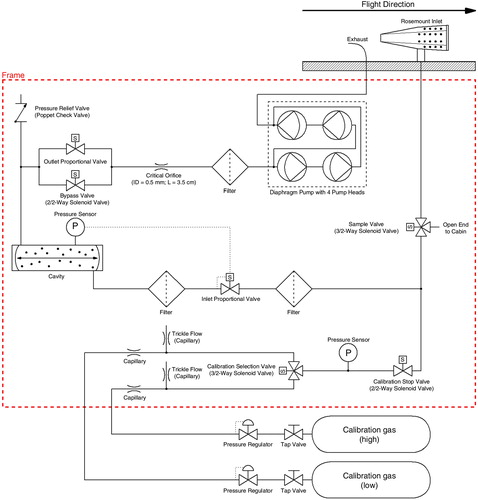
Table 1. Description of sub-assemblies and auxiliary parts

Part or assembly	Function/description
Frame	Aluminium box hosting all parts and providing the mechanical, electrical and pneumatic interface to the installation structure and to the calibration gas cylinders.
Functional parts
Cavity enclosure	Contains the sample cell (cavity). The enclosure is temperature controlled and set to T=45°C.
Wavelength monitor enclosure	Contains the wavelength monitor. The enclosure is temperature controlled. Setpoint is 45°C.
Vacuum pump	Provides the airflow through the instrument.
Laser system	The four channel analyser uses three telecom-grade distributed feedback lasers, mounted on similar diode laser electronic boards. Laser light is carried by fibre optics. A Semiconductor Optical Amplifier (SOA) amplifies the laser light before the measurement.
Calibration system	Controls three valves to calibrate the instrument with standard gas provided by the two high-pressure cylinders.
Thermo switches	Interrupt the electrical power provision to the whole instrument at temperatures above 70°C.
Auxiliary parts
Data acquisition system and power management	Circuit breaker; DC/DC converters for generation of 12V, −12V, 3.3V, 5V and 24V; Computer board to manage the data storage and handling the data transfer to the PI data interface; Power Board and Logic Board to control the subunits; SSD; AD-converter.

In order to provide uncontaminated ambient air to the instrument, it is equipped with an inlet line [3.18 mm (1/8″) OD Fluorinated Ethylene Propylene (FEP) tube, 60 cm], which is connected to a Rosemount Total Air Temperature (TAT) housing (model 102B; Stickney et al., 1994) mounted on the inlet plate at the fuselage of the aircraft. The Rosemount probe offers several advantages: it acts as a virtual impactor since the inlet line is pointed orthogonal to the airflow through the housing, and thus prevents from sampling larger aerosols (larger than about 2 µm), ice particles and water droplets; due to the strong speed reduction of the air it provides positive ram-pressure; and as standard housing for temperature and humidity sensors onboard civil aircraft it already possesses the required certifications (Fahey et al., 2001; Volz-Thomas et al., 2005). The additional positive ram-pressure of around 60 hPa at the ceiling level of 12.5 km, together with a low sample gas flow of 100 ml/min (100 sccm) (standard conditions for all given flows and volumes here and in the following: T=20°C, p=101 kPa) and the relatively short inlet line ensures operation of the instrument throughout the aircraft altitude operating range up to 12.5 km without an upstream sampling pump. Selection of the inlet line material (FEP) was made considering its suitability for the measurement of different species, as the IAGOS-core GHG system can be fully interchanged with the IAGOS-core NO/NO_x and NO/NO_y system and the characteristics of the material are particularly appropriate for these measurements. Given the short residence time of sample gas, the small inner surface area, the small mole fraction differences between ambient and cabin air and the low permeability of FEP, any impact from diffusion of CO₂, CH₄ and CO is minimal. The sample flow is exhausted through an exhaust line [6.35 mm (1/4″) OD FEP tube, 60 cm] connected to the exhaust duct included in the inlet plate.

The connection between Calibration Stop Valve and the tee-connector (see Fig. 1), which connects ambient air, calibration gas and the sample cell, is kept small [2.5 cm long 3.18 mm (1/8″) OD tube, 2 mm ID] to minimise the dead volume when measuring ambient/cabin air. Diffusion flow from the dead volume into the sample gas is <0.1% of the sample flow 30 s after switching from calibration to ambient/cabin sampling, and can thus be neglected.

To protect the sample cell from contamination, filters (Wafergard II F Micro In-Line Gas Filters, Entegris Inc.) are implemented. They also ensure thermal equilibration of the sample gas, as they are kept at the same temperature as the sample cell.

Pressure in the sample cell is controlled to 186.65 hPa (=140 Torr, variations of less than 0.04 hPa) with a proportional valve (‘inlet valve’) upstream of the cell, and the temperature is kept at 45°C (variations of less than 20 mK). Gas flow through the sample cell is controlled at 100 ml/min by a fixed flow restrictor (capillary) downstream of the sample cell and upstream of the pump. This capillary acts as critical orifice, as the pressure drops by more than a factor two between sample cell and pump. This makes the flow rate independent of ambient or cabin pressure. A pressure relief valve [set point 0.07 bar (1 PSIG)] protects the sample cell from accidental excess pressure.

Each species is measured once every 2.3 s. The physical exchange time of the sample cell is 3.6 s (volume=35 ml, sample flow=100 ml/min, pressure=186.65 hPa, sample temperature=45°C), ensuring that the ambient air is continuously sampled given the shorter measurement interval of 2.3 s.

The instrument has provisions to be connected to two fibre-wrapped aluminium cylinders (AVOX 897-94077 Cylinder and Valve Assembly, 17.1 l, max. filling pressure: 124 bar) filled with calibration gas. The connection to the outlets of the cylinder pressure regulators (AVOX 27660-19 Oxygen Regulator Assembly, sealing ring material: KEL-F81, membrane: silicon rubber) is made via coiled 1.59 mm (1/16″) OD stainless steel tubes equipped with quick connectors [Stäubli Tec-Systems GmbH, model RBE03, sealing: fluoric rubber (FPM)]. The quick connectors are sealed when not connected. During laboratory tests, it has been observed that the cylinder valves and pressure regulators can alter the composition of the calibration gas when the valves are open. For example, the pressure regulators were closed for different time spans and the gas composition was measured after they were opened again. It was found that already after 90 min of closing the CO₂ and CH₄ mole fractions at the beginning of the flushing period showed maximum deviations of more than 3 ppm, 4 ppb, respectively, from the final values, which were reached not until 30 min, 15 min respectively, of flushing. Such effects are known to be caused by permeation of CO₂ and CH₄ from the high- to the low-pressure side through polymer seal rings and by surface interaction effects (Sturm et al., 2004). Using theoretical calculations, the back-diffusion from the regulators into the cylinders was estimated to be <0.1 ml/min. Thus in order to eliminate back-diffusion and minimise the impact of the permeation and surface interaction effects in the regulator (in the following referred to as ‘regulator effects’), a trickle flow of 2.8 ml/min is applied to constantly flush the regulators.

2.3. Instrument operation

The measurement system operates fully automatically and without interruptions as long as the aircraft has power. The functions of the instrument are controlled by a single-board PC using Picarro Inc. measurement software.

Two operation modes are implemented to fulfil the different measurement requirements while the aircraft is in air (about 12 h/day, depending on the exact flight schedule) or on ground (about 8 h/day):

1. Ground Mode

   The instrument measures air from inside the frame (cabin air, i.e. outside air filtered by the air conditioning system) to protect the analyser from highly polluted air. Sample valve is off (see Table 2 and Fig. 1). High frequency of calibrations enabled.

2. Flight Mode

   Ambient air is measured and the calibration frequency is lower than on the ground.

To switch between ground and flight modes, the WoW signal from the aircraft is used. In the laboratory, the instrument can be operated in ground mode, flight mode and manual mode, where all valves and I/O functions can be switched individually.

Table 2. Valve selection for different instrument modes

Instrument mode	Sample valve (off=cabin air)	Calibration stop valve	Calibration selection valve
Ground mode	Off	Off	Off
Calibration tank I (on ground)	Off	On	Off
Calibration tank II (on ground)	Off	On	On
Flight mode	On	Off	Off
Calibration tank I (during flight)	On	On	Off
Calibration tank II (during flight)	On	On	On

The instrument is calibrated at regular intervals by measuring calibration gas provided by two fibre-wrapped aluminium cylinders. Each cylinder contains dried ambient air, but with different CO₂, CH₄ and CO concentrations (high-span and low-span). With the help of three valves (sample valve, calibration stop valve, calibration selection valve; GEMS Sensors Inc., G- & GH-Series) the gas flow through the measuring cell can be switched between calibration gas and air from the inlet respectively in the cabin, as can be seen in Fig. 1 and Table 2.

The calibration gas flow is maintained by capillaries acting as flow restrictors with an upstream pressure regulated to 570–670 kPa (5.7–6.7 bar, depending on the cylinder pressure and cabin pressure) with pressure regulators. This pressure is monitored with a pressure sensor in the calibration gas line (GCT-225 model, Synotech GmbH). Calibration gas flow is kept above 110 ml/min, ranging up to 165 ml/min with nearly empty cylinders and at lowest cabin pressure (800 hPa), and thus higher than the normal sample flow (100 ml/min). During calibration, the excess flow of at least 10 ml/min leaves the system backwards through the inlet to ensure that no air from outside is entering the system.

Although small variations in sample gas flow have no impact on the measurements, it is important to monitor the flow as it affects the exchange rate of the sample gas. When the instrument switches between ambient air, cabin air, or calibration gas measurement, time passes until the change in signal occurs. The flow is inversely proportional to this lag time and can be calculated if the inner volume of the flushed tubing is known. To allow a regular determination of the sample flow, the ‘open end to cabin’ in Fig. 1 is realised as a 1.3 cm (0.5″) ID tube with a length of about 22 cm. Thus, the lag time when switching from calibration gas to cabin air during ground operation is extended, which together with the cabin pressure measurement allows monitoring the flow with ~5% accuracy.

For reporting dry air mole fractions, the system requires no drying of the sample air, as the simultaneously measured water vapour mole fraction is used to correct for dilution and spectroscopic (pressure-broadening) effects. The parameters of this wet-to-dry correction are based on laboratory experiments made with each IAGOS-core GHG instrument during each maintenance cycle, i.e. every 6 months, as this method has been shown to result in the lowest uncertainty in the water vapour correction (Chen et al., 2013; Rella et al., 2013).

Further tests will be made before the first deployment regarding the implementation of an updated software parameter, affecting the transition time between wet and dry measurements, to avoid artificial gradients between wet and dry air, e.g. boundary layer and free troposphere, or troposphere and stratosphere (Karion et al., 2013).

3. Laboratory tests

To prepare the IAGOS-core GHG instrument for deployment onboard commercial aircraft and ensure a reliable performance of the analyser, tests in the laboratory were conducted to assess airworthiness and measurement characteristics, detect functional limits and develop needed corrections.

3.1. Instrument response stability

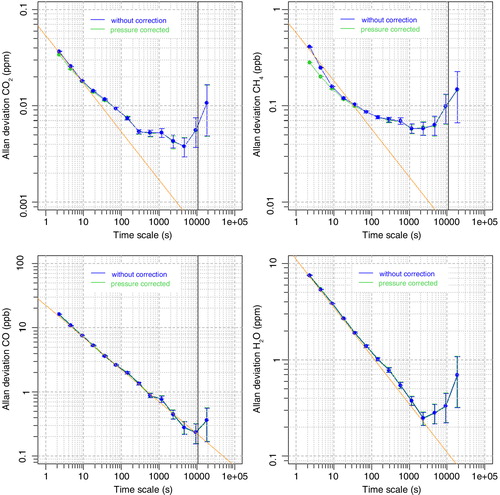
To assess the long-term stability of the measurement system and design an initial calibration strategy (particularly calibration frequency), dried ambient air from a high-pressure tank was measured continuously for 24 h. The first 3 h were removed to ensure dry and stable conditions. Analysis of the data by Allan variance technique (Allan, 1966, 1987), using the R-package ‘allanvar’, determined the standard deviations of the raw 0.4 Hz data as 0.039 ppm for CO₂, 0.40 ppb for CH₄ and 15 ppb for CO. As can be seen in the resulting Allan deviation plots (see Fig. 2, blue data points) the CO and water vapour signals are, at a timescale of ~10 000 s, dominated by white noise (green line), while for CO₂ and CH₄ also other effects, e.g. drift, are an issue. Since random errors are uncorrelated, precision of the CO measurements can be reduced by applying temporal integration. Passenger aircraft travel approximately 1 km horizontal and 30 m vertical in 4 s. Therefore, an integration time of 3 min, reducing the precision to 1.7 ppb, would be sufficient for global and regional atmospheric models with typical horizontal resolutions of around 50–100 km. To eliminate drift impact on the CO₂ and CH₄ measurements, calibrations are needed. The Allan variances shown here are obtained under laboratory conditions and it needs to be assessed during the first flight period if they can be achieved under flight conditions, too. Therefore, a conservative initial frequency of three-hourly calibrations (every 10 800 s) during flight is chosen, which allows for at least two calibrations per flight. On ground, an even higher frequency with two-hourly calibrations is chosen, to utilise the time where no measurements are made for detailed drift analysis.

Fig. 2 Allan deviation plots of a 21-h measurement of dried, ambient air from a high-pressure tank for CO₂, CH₄, CO and H₂O. The raw measurement data are shown in blue, data corrected for sample cell pressure deviations in green. The orange line (slope −0.5) shows the region of Gaussian or white noise. The black vertical lines at 10 800 s (3 h) indicate the planned calibration frequency.

3.2. Calibration tests

The fully automated calibration system was tested in the laboratory by executing a typical measurement cycle during deployment of the instrument onboard aircraft with alternating measurements of ambient air (during flight), respectively cabin air (on ground) and calibration gas. Trickle flow was adjusted to 2.8 ml/min. The ‘Weight on wheels’ signal from the aircraft was simulated with a mock-up to switch between ground and flight modes and hence between different calibration sequences (3 hourly in air, 2 hourly on ground). A calibration consisted of a high-span and a low-span measurement of 10 min each, whereby the measurement order was swapped every other calibration.

Figure 3 shows a single, low-span calibration measurement during the simulation. After starting the calibration, a distinct delay for CO₂ (black points) and CH₄ (dark green points) and H₂O (blue line) can be observed until the measurement is stable. For water vapour, this is caused by the switch from wet ambient/cabin air to dry calibration gas, and by desorption of H₂O from the walls of the inlet line downstream of the sample valve. For CO₂ and, to a lesser extent for CH₄, the main reasons for this “transition effect” are diffusion and surface interaction effects in the pressure regulator of the calibration gas cylinder, mainly preferential permeation of CO₂ through sealing rings (membrane: silicon rubber; Sturm et al., 2004). The transition time from wet to dry gas related to the slow update of the CO₂ and CH₄ baselines in the Picarro measurement software (Karion et al., 2013) is not important here, since this effect is small and of shorter duration compared to the regulator effects. For CO, the measurement variability is too high to see any transition effects.

Fig. 3 Low-span calibration measurement (CO₂ – black, CH₄ – light green, CO – yellow, H₂O – blue) during simulation of a typical measurement cycle with a trickle flow of 2.8 ml/min. ‘Time’ is the time after the calibration was started in minutes. For CO₂ and CH₄ exponential fitting curves to the calibration time series are shown in grey and light green, respectively.

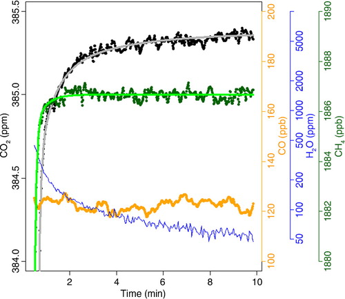
Since the amount of calibration gas is limited and needs to last for a full 6-month deployment period, the duration of each calibration needs to be limited. However, especially the measured CO₂ signal might not yet have reached the final value at the end of the calibration cycle. To reduce the impact from non-equilibrium calibration gas measurements, a fit procedure is applied to each calibration measurement to estimate the equilibrium values for dry air mole fraction for each calibration gas (grey line for CO₂, light green line for CH₄). For this, a combination of exponential functions is used:1 Here, X is the mole fraction, t the time and t ₀ the starting time of the calibration plus 30 s. The first 30 s of a calibration are removed to allow for some initial flushing. The number of exponential functions used varies between one and three depending on the species. The parameters X _equilibrium, a _i and τ _i for the different species are determined by fitting an averaged time series of all 10-min calibration cycles (six low-span calibrations+six high-span calibrations) performed in the laboratory. This procedure is possible since tests with different calibration frequencies (from hourly to daily) and different mole fractions of the previous measurements (350–420 ppm for CO₂, 1600–2000 ppb for CH₄, 20–300 ppb for CO) indicated, that the characteristics of the calibration time series are reproducible and nearly independent of the different calibration frequencies, and the difference in mole fraction to the previous measurement (after accounting for the 30 s flushing time). After the average temporal characteristic of the transition effect is captured with eq. (1), the following equation is used to fit each individual calibration:2 Here, a correction c _j to the equilibrium mole fraction X _equilibrium and a factor b _j to scale the sum of the exponential functions are adjusted.

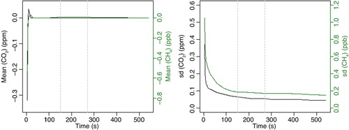
To assess to which degree this procedure allows for reducing the length of a calibration, eq. (2) was fitted to each individual time series of the above mentioned 10-mine calibrations, whereby the length of the time interval used for fitting was varied between 4 and 560 s. Figure 4 shows the mean and the standard deviation of the 12 fitted correction factors c _j for CO₂ and CH₄ depending on the time span used for the fit, i.e. the calibration length minus 30 s flushing. While the mean is not changing any more after around 30 s (variations of >0.005 ppm for CO₂ and 0.01 ppb for CH₄), the standard deviations still decrease. After 150 s (calibration length of 3 min) the standard deviation for CO₂ (CH₄) is 0.07 ppm (0.19 ppb), after 270 s (5 min calibration length) it is 0.05 ppm (0.17 ppb). Compared to a 10-min long calibration, this means an increase in the standard deviation, and thus an increase in the uncertainty of the correction factor c _j , of 0.03 ppm for CO₂ (0.04 ppb for CH₄) for a calibration length of 3 min, and of 0.01 ppm (0.03 ppb) for a calibration length of 5 min. This procedure will be regularly re-assessed during maintenance.

Fig. 4 Mean and standard deviation (SD) of the eight fitted corrections c _j for CO₂ and CH₄ as a function of the time interval used for fitting the calibration measurement. ‘Time’ is the time after 30 s flushing. The grey vertical lines indicate 3- and 5-min calibration lengths (150 and 270 s, respectively).

For CO, the experiments showed that no fit procedure is needed and the calibration gas measurement is obtained by averaging the measurement data, after discarding the first 30 s.

3.3. Pressure test

During flight, the instrument faces a wide range of ambient pressures at the air inlet and outlet. Air pressure decrease during ascent varies from 100 hPa/min at lower altitudes (0–3 km, corresponding to 1000–700 hPa) to 10 hPa/min at higher altitudes (9–12 km, corresponding to 300–200 hPa). Similarly, pressure increase during descent lies between 100 and 20 hPa/min for lower and higher altitudes, respectively. At ceiling level (approximately 12 km), the inlet pressure drops to about 250 hPa. This is higher than the real ambient pressure at that height since the Rosemount inlet provides additional ram-pressure of around 60 hPa. For the backward-facing air-outlet negative ram-pressure has to be taken into account, which leads to outlet pressures down to about 130 hPa at ceiling level. To assure that the sampling pump downstream of the sample cell can cope with the low pressure conditions and keep the sample flow stable at 100 ml/min and that the pressure adjustment in the sample cell is fast enough to compensate for the strong pressure gradients, parameters of the pressure control loop were adjusted and an appropriate test was performed in the laboratory. Pressure at the outlet was lowered with the help of an additional pump downstream of the instruments pump, with a needle valve in between to adjust the pressure. To achieve the required inlet pressure variations, gas was provided to the instrument with an excess flow, which was lowered in pressure by a further pump, using a buffer volume and a needle valve for pressure control.

Figure 5 shows a complete pressure cycle including an ascending and descending flight profile with typical pressure gradients. Sample flow (in green) is nearly stable at 104 ml/min throughout the whole test with only small deviations during ascent (−2 ml/min) and descent (+2 ml/min) which are caused by the required pressure equilibration in the inlet line. This confirms the good performance of the sampling pump also at low ambient pressures. Pressure in the sample cell (in blue) is stable at its setpoint of 186.65 hPa (dark blue line) when the inlet pressure is stable regardless of whether the actual pressure is high or low. During normal changes of the inlet pressure, like they occur during flight, the sample cell pressure shows small deviations up to 0.03 hPa. Only for large changes in inlet pressure at pressure levels lower than 300 hPa (changes by 40 hPa/min, see minute 26), the sample cell pressure deviation peaks at 0.15 hPa, indicating that the sample cell pressure adjustment is too slow to adapt.

Fig. 5 Typical pressure changes during flight profile measurements. Shown are the 30 s means of the pressure at the air inlet (in grey) and the air outlet (black), pressure in the sample cell (blue) and sample flow (green). The vertical dark blue line indicates the setpoint of the sample cell pressure at 186.65 hPa (corresponding to 140 Torr).

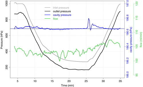
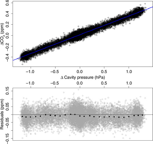
Since the measurements of the instrument are calibrated at a sample cell pressure of 186.65 hPa, deviations in sample cell pressure result in erroneous GHG measurements due to changes in dilution and pressure-broadening effects with changing cell pressure. While dilution leads to higher signals with higher sample cell pressure, for pressure broadening it is the other way round. Figure 6 shows the deviation in the observed CO₂ signal due to pressure deviations in the sample cell, measured at a CO₂ mole fraction level of 390 ppm. The use of a linear fit (blue line) allows for a correction of the measurements. The correction factor (slope of the linear fit) is 0.35 ppm/hPa for CO₂, 6.18 ppb/hPa for CH₄ (at a CH₄ mole fraction level of 1920 ppb) and −2.1 ppb/hPa for CO (at a CO mole fraction level of 150 ppb). The negative correction factor for CO is likely due to a relatively stronger effect from pressure broadening than dilution for CO. Residuals of the raw CO₂ data can be seen in grey, the black points are mean values for sample cell pressure intervals of 0.1 hPa. It is obvious that the noise of the raw data is much larger than the actual correction. To assess quantitatively how much extra noise the sample cell pressure correction adds to measurement data, the data of the response stability test (Section 3.1) were pressure corrected using the raw 0.4 Hz sample cell pressure data, and the Allan variance was recomputed. The Allan Deviation plots in Fig. 2 show the results for the uncorrected and the corrected data. The standard deviation of the corrected 0.4 Hz measurement data is decreased by 0.002 ppm for CO₂ and 0.1 ppb for CH₄ compared to the uncorrected values, while for CO and water vapour no changes were observed. This means that applying the sample cell pressure correction to the measurement data has no negative impact on the data quality.

Fig. 6 Error of the CO₂ measurement due to deviations in sample cell pressure referenced to the setpoint of 186.65 hPa (140 Torr), measured at a CO₂ mole fraction level of 390 ppm. The blue line is a linear fit of the data. The correction factor (slope of the linear fit) is 0.35 ppm/hPa for CO₂, 6.18 ppb/hPa for CH₄ (at a CH₄ mole fraction level of 1920 ppb) and −2.1 ppb/hPa for CO (at a CO mole fraction level of 150 ppb). Residuals are shown in grey, black points are the mean values for intervals of 0.1 hPa sample cell pressure.

3.4. Airworthiness tests

To assess the risks regarding mechanical and electrical performance (physical damage by loose or broken parts, EMI with the electronic system of the aircraft, exposure to abnormal power supply), the instrument was tested according to a specified qualification programme. Vibration and shock tests have been applied for all three orthogonal axes of the analyser. After the tests, no mechanical damages of the system have been detected. Tests concerning power input and voltage spikes, as well as EMI tests for conducted and radiated EMI proved that no inferences could adversely affect other aircraft systems.

After completing these qualification tests, the instrument was installed and tested in the first IAGOS equipped aircraft (Lufthansa D-AIGT) in May 2013. This ‘Ground Test’ included a general design inspection of the instrument as well as functional tests, and the absence of EMI with other aircraft systems was checked. The analyser passed all tests.

4. Calibration strategy

A single deployment period of the instrument in the frame of the IAGOS project lasts for approximately 6 months. The exact number of days depends on the maintenance schedule of the aircraft set by the airline. To ensure traceability of the IAGOS-core GHG measurements to the WMO primary scales, the calibration strategy includes measurements of standards traceable to the primary scale before and after the deployment period (‘pre- and post-deployment calibration’), as well as regular measurements of calibration gas during the deployment (‘In-flight calibrations’). When determining frequency and length of the in-flight calibrations, it has to be considered that the amount of calibration gas during one deployment period is limited by the size of the two gas cylinders (each with a capacity of 1600 standard litres of gas, which can be used for the calibrations) carried along.

4.1. CO₂, CH₄, CO

Traceability of the CO₂, CH₄ and CO measurements to the WMO primary scales [currently WMO X2007 scale for CO₂, WMO X2004 scale for CH₄, WMO X2014 scale for CO (WMO GAW report 206, 2012)] is ensured in a multi-step procedure:

During the 6-month deployment of the instrument aboard aircraft regular calibration takes place by measuring pressurised standard air from two calibration gas cylinders (mole fractions for CO₂, CH₄ and CO of approximately 375 ppm, 1700 ppb, and 70 ppb for the low and 400 ppm, 1900 ppb and 150 ppb for the high cylinder; ‘in-flight calibrations’). Since the analyser detects only the most abundant isotopologue of each trace gas, standards were prepared with similar isotopic composition to that found in ambient background air. While the aircraft is on the ground, more frequent and longer calibrations will be made than during flight to ensure an optimal usage of measurement time in air. The first calibration on ground will always start 30 min after power is switched on to allow enough time for the warming phase of the instrument. After short power interruptions of some minutes, e.g. when the aircraft switches from self-power to gate-power and vice versa, the warm-up lasts for around 5 min. If the aircraft is parked longer without power supply, the warming phase takes longer. In air, the first calibration is scheduled after 1 h. That way no calibration takes place during ascent such that a full profile measurement is achieved. Nevertheless, after half-a-year deployment with usually two long-range flights per day and because of the different flight durations enough calibrations will be performed at all altitudes during descent so that any potential pressure effects can be detected. After landing, a calibration will be started immediately to assure that at least one calibration cycle is finished before power is shut off, when switching from self- to gate-power.

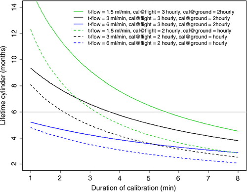
Figure 7 shows the lifetime of a calibration gas cylinder filling depending on the duration and number of in-flight calibrations and the trickle flow rate, which is used to constantly flush the regulator and thus minimise the impact of regulator effects. While a long calibration time and a large trickle flow reduce the uncertainty of the calibration gas measurement, a more appropriate drift correction can be achieved by a higher calibration frequency. As a compromise, in order to reach 6-month lifetime of the cylinder filling, a trickle flow of 3 ml/min and a 3 hourly calibration frequency during flight, 2 hourly on ground, with 3 and 5 min duration of the calibrations in air and on ground, respectively, appears to be a suitable approach. It will be reviewed as soon as the first real flight data are available. Especially an envisioned 3-month test phase, which will allow for more frequent and longer calibrations, will be used to verify the calibration strategy.

Fig. 7 Lifetime of a calibration gas cylinder filling for various calibration scenarios. t-flow stands for trickle flow, cal@flight(ground) is the calibration frequency during flight (on ground). The grey horizontal line indicates a lifetime of 6 months.

After the deployment period, the calibration gas cylinder assembly (cylinders, pressure regulators, tubing) and the instrument get re-calibrated at the Max Planck Institute for Biogeochemistry (MPI-BGC) with the help of three working standards (‘post-deployment calibration’). These working tanks are filled with pressurised, dried ambient air at the GasLab of the MPI-BGC and are measured against calibrated reference gas mixtures (tertiary standards) provided by the WMO Central Calibration Laboratory (CCL) that maintains the primary scale. The in-house tertiary standards are regularly (every 3–5 yr) recalibrated by the CCL. CCL for all three species (CO₂, CH₄, CO) is NOAA/ESRL. The flow diagram in Fig. 8 illustrates the calibration chain of the CO₂, CH₄ and CO measurements.

Fig. 8 Calibration chain of the IAGOS-core instrument ensuring the traceability of the measurements to the World Meteorological Organization primary scales.

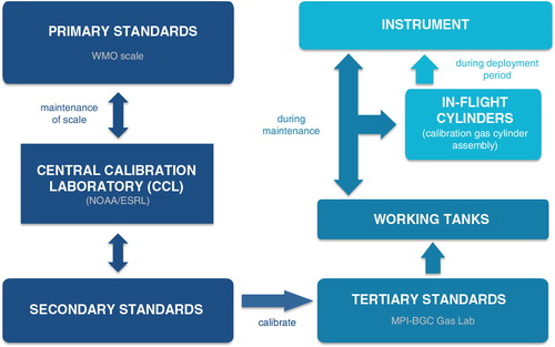
After the post-deployment, calibration and maintenance the calibration gas cylinders are refilled and the calibration gas cylinder assembly and the instrument are calibrated again with the help of three working standards traceable to the respective primary scales (‘pre-deployment calibration’). Later, instrument and cylinders are shipped for a new deployment period.

A settling time of 2 weeks between filling and measuring the calibration gas cylinders ensures that a representative measurement of the gas can be made, as experience with the first set of calibration gas cylinders indicated. Hence, the cylinders might be replaced by a different set for the next flight period depending on the time schedule.

During both, pre- and post-deployment calibrations, the same pressure regulators for the in-flight calibration gas cylinders are used as during flight operation. This minimises impact from potentially different effects on CO₂ from different regulators (i.e. with a different serial number). To reduce impact from wall effects in the calibration gas cylinders (release of CO₂ bound to the cylinder walls), the final pressure (at the end of the post-deployment calibration) is kept above 3 MPa (30 bar; Daube et al., 2002).

The role of the in-flight calibrations in the data processing will be assessed as soon as first data are available. Possible options: fully rely on each individual in-flight calibration; fully rely on the linear drift of the instrument between the pre- and post-deployment calibrations in the laboratory; or a mixture of both options, e.g. only a temporal average of the in-flight calibrations is used for the correction, as described by Karion et al. (2013).

The data management system allows for easy reprocessing and propagation of scale changes from the secondary standards to the final measurements.

4.2. Water vapour

Currently, the water vapour measurements are not calibrated regularly against a reference standard that is traceable to the primary scale. For the initial water calibration of the instrument, the calibration constants of a similar instrument (G1301-m, Picarro Inc.) calibrated at MPI-BGC Jena against a dew point mirror [Dewmet, Cooled Mirror Dewpointmeter, Michell Instruments Ltd., UK, referenced to National Institute of Standards and Technology (NIST)] in the range from 0.7 to 3.0% were transferred to all subsequently manufactured CRDS instruments by Picarro Inc. (Winderlich et al., 2010). A procedure to ensure proper traceability is under development.

5. Uncertainty analysis

The current uncertainty analysis of the IAGOS-core GHG instrument measurements is based on laboratory tests and test flights on a research aircraft, since the instrument is not yet operational. For the first installation of the instrument aboard passenger aircraft, a 3-month test phase is envisioned. This will allow for detailed checks of all instrument functions, more frequent and longer calibrations than during normal 6-month deployment periods, and a review of the overall uncertainties. An up-to-date detailed uncertainty analysis will be provided and regularly updated in the document ‘Standard Operation Procedure for the IAGOS-Core GHGs Instrument (P2d)’ at the IAGOS database (www.iagos.org). Final data, stored at the database, include individual uncertainty components (e.g. from calibrations, wet-to-dry correction, isotopic effects) for every observation. These time-dependent uncertainty estimates will for CO₂, CH₄ and CO include effects from varying water vapour content, varying mole fractions (relative to the calibration range set by the low-span and high-span gases), and possibly effects rising from different ambient pressure. In the following, we discuss conservatively estimated uncertainties, but for mole fractions within the calibration range.

5.1. CO₂, CH₄, CO

Table 3 shows the different contributions to the overall uncertainties of the CO₂, CH₄ and CO measurements. The individual components concern the referencing of the in-flight calibration gases to WMO primary standards, but uncertainty in the conversion of observed wet mole fractions to dry air mole fractions is also included. Instrument response drift is compensated by regular calibrations. As the steps in calibration transfer are independent from each other, and independent of the uncertainty introduced by the wet-to-dry correction, propagation of uncertainties is made assuming that all contributions are independent (Gaussian error propagation assuming independent variables). Only the bias for isotopic effects is added linearly.

Table 3. Estimates of the different uncertainty components for the IAGOS-core CO₂, CH₄ and CO measurements and the resulting overall uncertainties (1-sigma)

Uncertainty contributions	CO2	CH4	CO
MPI-BGC GasLab implementation of the WMO primary scale	0.015 ppm	0.7 ppb	0.5 ppb or 0.25% (whichever is greater)
Calibration transfer to the laboratory working tanks	0.02 ppm	0.15 ppb	0.7 ppb or 0.4% (whichever is greater)
Calibration transfer from the working tanks via in-flight cylinders to the instrument	0.07 ppm	0.28 ppb	2.8 ppb
Drift correction of the in-flight cylinders and regulator effects	0.05 ppm	–	–
Isotopic composition	0.019 ppm	–	–
Wet-to-dry correction	0.05 ppm	1 ppb	2 ppb
Measurement repeatability	0.039 ppm (2.3 s time resolution)	0.40 ppb (2.3 s)	1.7 ppb (3 min time resolution)
Achieved overall uncertainty (1-sigma)	0.13 ppm	1.3 ppb	4 ppb
WMO/GAW compatibility goal	0.1 ppm/0.05 ppm (northern/southern hemisphere	2 ppb	2 ppb

Also listed are the GAW compatibility goals for comparison.

MPI-BGC GasLab implementation of the WMO primary scale for CO₂ covers uncertainty of the NOAA secondary standards (0.014 ppm; Zhao and Tans, 2006) and tertiary standards (0.014 ppm). The MPI-BGC GasLab has seven tertiary standards available and thus, the uncertainty of the BGC-GasLab implementation of the WMO CO₂ primary scale can be calculated using the following equation:3 For CH₄, an uncertainty of the WMO tertiary standards of 0.7 ppb is assumed (Dlugokencky et al., 2013). This tertiary standard set includes standards at non-ambient mole fractions, which might be slightly biased, such that 0.7 ppb is taken as uncertainty of the MPI-BGC GasLab implementation of the WMO CH₄ primary scale. For CO, uncertainty of tertiary standards is adopted from the GAW Report No. 206 (WMO, 2012).

CO₂ and CH₄ calibration of the laboratory working tanks is made at the MPI-BGC GasLab using a CRDS analyser (G1301, Picarro Inc.), CO calibration using a vacuum ultraviolet resonance fluorescence (VURF) analyser (Aerolaser AL 5002). Each of these instruments is calibrated by working standards that are assigned relative to the above-mentioned suite of WMO tertiary standards. The uncertainty of the calibration transfer at MPI-BGC GasLab comprises the uncertainty of the GasLab working standard assignment (including its stability over time) and the reproducibility of the analytical method to assign the IAGOS working tanks.

The CRDS instrument is calibrated daily using three GasLab working standards spanning the atmospheric range of CO₂ and CH₄. The reproducibility of assignments of these standards for multiple calibration episodes relative to the WMO tertiary standard suite (ca. 10 episodes per working standard) is 0.01 ppm for CO₂ and 0.1 ppb for CH₄, respectively. Within this series of re-calibrations, drifts of CO₂ mole fractions of 0.01–0.015 ppm/yr have been detected in several working standards. A linear drift function is applied in these cases. In contrast, all working standards have been stable in their CH₄ mole fraction. Thus, the uncertainty of the CH₄ scale transfer to the GasLab working standards is corresponding to the standard error of 0.03 ppb (0.1 ppb/), whereas the uncertainty of the CO₂ scale transfer is approximated as 0.01 ppm.

The accuracy of the GasLab assignments of IAGOS working tanks is assessed based on the time series of daily target standard measurements. The standard deviation of these daily mean values is 0.015–0.02 ppm for CO₂, and 0.1–0.2 ppb for CH₄ for a 20-min measurement period. These long-term quality control records do not only represent the analysers precision but also additional disturbances apparent in the laboratory operation (e.g. temporary small leakages). Combining the uncertainty of the GasLab working standard assignment and the general reproducibility of the analytical method yields a total MPI-BGC GasLab scale transfer uncertainty of 0.02 ppm for CO₂ and 0.15 ppb for CH₄.

For the VURF CO-analyser, a one-point calibration using a single working standard and a zero gas analysed each for 6 min is made every 30 min. The relative reproducibility of working standard assignments relative to the WMO tertiary standard suite (six episodes per working standard) is 0.2% (0.4 and 0.8 ppb for two working standards at 246 and 426 ppb, respectively). The first working standard showed a steady increase of CO mole fractions at a drift rate of 0.6 ppb/yr that was accounted for using a linear interpolation. Similarly, one of the standards in the GasLab CO WMO tertiary standard set showed a CO growth of 1 ppb/yr and therefore has not been used for calibration. This points to a potential bias of the tertiary set due to a similar drift of the entire set as it has been reported by the WMO-CCL for CO in some primary standards at a rate of 0.3 ppb/yr (see www.esrl.noaa.gov/gmd/ccl/co_scale.html). Recent re-calibrations at the WMO-CCL of two tertiary standards, however, did not indicate any CO growth over a period of 9 yr. Absolute values of the residuals of the seven tertiaries with CCL assignments obtained in different years since 2005 are less than 0.5 ppb with no systematic trend in the time series of residuals of any single standard. Based on this evidence, it is assumed to be unlikely that the MPI-BGC GasLab tertiary standard suite comprises any bias due to instabilities in the standard CO mole fractions. This is consistent with the absence of any significant drift in the time series of target standards. However, despite the absence of a clear indicator for drift of the GasLab tertiaries an upper limit of 0.5 ppb for the stability of the set is taken as conservative estimate for the uncertainty of the tertiary assignments considering the known problems with CO growth and the associated challenge of detecting small drifts. Accounting for this uncertainty, a relative calibration transfer uncertainty of the GasLab working standards of 0.3% is derived for the working standard containing 246 ppb CO. Target standards are analysed daily in the same way as the IAGOS working tanks (15-min measurement period divided by a calibration). The record of these target standard measurements documents a long-term relative reproducibility of the VURF CO analysis of 0.25%. By combining the uncertainty of the MPI-BGC GasLab working standard assignment and the reproducibility of the analytical method, the MPI-BGC GasLab scale transfer uncertainty for CO is estimated as 0.4% relative or 0.7 ppb absolute (whichever is greater).

The last step of the calibration chain is the calibration of the IAGOS-core GHG instrument with the help of the working tanks and the in-flight calibration gas cylinders. Here, the repeatability of the instrument for the measurements of the working tank calibration gases and the in-flight calibration gases is deduced from laboratory experiments as 0.015 ppm for CO₂, 0.15 ppb for CH₄ and as 2 ppb for CO. For the in-flight calibrations the uncertainty of the free parameter c _j in eq. (2) has to be added to the measurement uncertainties for CO₂ and CH₄. Table 3 assumes the worst case, where instrument drift needs to be compensated for by 3-hourly calibrations. In the best case, the instrument does not drift significantly, and all calibrations (pre-, post- and all in-flight calibrations) can be statistically combined, which reduces the uncertainty significantly. For now, without flight experience, the worst-case scenario is considered for the calculations to give an upper limit of the uncertainty. The uncertainty of the parameter c _j for 3-min calibrations is 0.07 ppm for CO₂ and 0.19 ppb for CH₄ (see Section 3.2). By combining the repeatability of the working tank measurements and the in-flight calibration gas measurements with the uncertainty of the parameter c _j , the overall uncertainty of this calibration transfer step is determined as 0.07 ppm for CO₂, 0.28 ppb for CH₄ and 2.8 ppb for CO. For the best-case scenario, the uncertainty would be 0.015 ppm for CO₂, 0.15 ppb for CH₄ and 2 ppb for CO.

Uncertainty due to drift correction of the in-flight calibration gas cylinders and due to regulator effects [e.g. parameters in eqs. (1 and 2) determined beforehand change over time and in particular with decreasing tank pressure] is for now only estimated and will later be based on experience from operational QA/QC cycles. As known from experience, in-flight calibration gas cylinder drift and regulator effects are very small for CH₄, for CO they are small in relation to the uncertainty introduced by calibration transfer and instrument repeatability, respectively. Therefore, uncertainty due to these effects is assumed to be negligible for CH₄ and CO.

The CO₂ isotopic composition in the calibration gases is kept close to that of ambient air (−12‰>δ¹³C _VPDB>−8‰, 0‰>δ¹⁸O _VPDB>7‰). Due to differences in the isotopic signature of CO₂ between the tertiary standards calibrated by the CCL and the laboratory working tanks (filled with the calibration gases), small measurement biases of maximal 0.019 ppm at 400 ppm level occur. Any further measurement bias from differences in the isotopic composition of the working standards and the in-flight standards can be excluded as their assignment is done with the same analytical technique. Measurement errors caused by deviations of the calibration gases in the isotopic composition of CH₄ were found to be negligible as the fraction of these deviations to total methane is small; in addition the measured biases due to ¹³C and deuterium compensate each other. For CO the isotopic composition is not known, but estimations based on similar values as for CO₂ are insignificant compared to the measurement repeatability.

The wet-to-dry correction is based on laboratory experiments made with each instrument during each maintenance cycle. Thus, the smallest uncertainties can be achieved as described in Rella et al. (2013) for CO₂ and CH4 and Chen et al. (2013) for CO. With the experience of repeated wet-to-dry experiments in the laboratory over a long period, the uncertainty estimates will be optimised.

Measurement repeatability of the instrument is given at 2.3 s time resolution for CO₂ and CH₄; for CO an integration time of 3 min is applied (see Section 3.1).

Propagation of all these uncertainty contributions (Gaussian error propagation assuming independent variables, bias due to isotopic composition added linearly) results in an overall uncertainty (1-sigma) of the IAGOS-core GHG measurement system of 0.13 ppm for CO₂, 1.3 ppb for CH₄ and 4 ppb for CO. A less conservative assumption of instrument drift in the third step of the calibration chain (calibration transfer from the working tanks via in-flight cylinders to the instrument) results in overall uncertainties of 0.10 ppm for CO₂, 1.3 ppb for CH₄ and 3.4 ppb for CO. The uncertainty estimates are in good agreement with the overall uncertainty (0.15 ppm for CO₂, 1.4 ppb for CH₄, 5 ppb for CO) of the similar CRDS measurements made by Karion et al. (2013). Note that the WMO GAW compatibility goals shown in Table 3 should actually represent most upper limits, as individual measurement programmes should strive for significantly smaller uncertainties. However, the fact that those are likely not met for CO₂ and CO indicates that this is hard to achieve with aircraft measurement programmes.

5.2. Water vapour

For water vapour, the overall uncertainty includes an instrument response drift of <100 ppm or <0.5% (whichever is greater) over 6 months and traceability to the NIST (Gaithersburg, MD) scale. Uncertainty of the calibration transfer from NIST scale to the instrument is 0.2°C dewpoint at 20°C dewpoint, linearly increasing to 0.4°C dewpoint at −60°C dewpoint, corresponding to the specifications of the Cooled Mirror Dewpointmeter from Michell Instruments used for calibration. A conservative estimate of the measurement repeatability is 4 ppm for mole fractions<100 ppm, and 4% (relative) for mole fractions>100 ppm (see Section 6). The resulting overall uncertainty (1-sigma) of the water vapour measurements for the different measurement ranges can be seen in Table 4.

Table 4. Overall uncertainty (1-sigma values) of the water vapour measurements

Measurement range	Achieved overall uncertainty
<100 ppm	<15 ppm
100–300 ppm	<25%
300–1000 ppm	<11%
1000–10 000 ppm	<6%
>10 000 ppm	<4%

6. Flight test – DENCHAR flight campaign

In May–June 2011, the gas analyser (G2401-m, Picarro Inc.) was tested, as it was purchased before being repacked, in a flight campaign based in Hohn (Germany). This inter-comparison campaign was conducted within the framework of the DENCHAR (Development and Evaluation of Novel Compact Hygrometer for Airborne Research) project, funded by the European Facility for Airborne Research (EUFAR), to compare well-established reference instruments with newly developed systems measuring water vapour. During the inter-comparison campaign, four flights with a Learjet 35A took place in an area between North-Germany and South-Norway and North-Poland and the North Sea respectively. Altidues up to 13 km were reached, hence also the lower stratosphere was covered.

Since the CRDS analyser and the inlet system components, a 1 m-long 3.18 mm (1/8″) FEP-tube connected to a Rosemount TAT housing (model 102BX) installed on a window plate of the Learjet, are identical to those in the repacked IAGOS-core GHG package this test setup ensures full comparability with the deployment of the analyser within IAGOS.

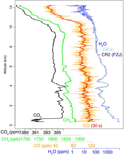
Figure 9 shows a profile for each species measured during the campaign at noon on 1 June 2011. The steep gradient at approximately 800 m indicates the mixing height covering the planetary boundary layer. At approximately 10 km, the aircraft crossed the tropopause which can be clearly seen by the strong decrease in the mole fractions of all four species with altitude, characteristic for the lower stratosphere.

Fig. 9 Measured profiles (0.4 Hz data) by the CRDS analyser during noon on 1 June 2011 over Hohn (Germany) for CO₂ (black), CH₄ (green), CO (orange, 30 s average in red) and H₂O (blue, 30 s average in light blue). The measurements from the frostpoint hygrometer CR2 can be seen in dark blue.

Upper limits for the measurement repeatability of the instrument during the test flights were determined during time periods with stable atmospheric conditions. The results are shown in Table 5. Note that the time resolution during the flight test campaign (2.5 s) was different to the laboratory tests (2.3 s) due to small modifications to the instrument after the flight test.

Table 5. Upper limits of the measurement repeatability during the DENCHAR flight campaign

Species	Time resolution	Measurement repeatability
CO2	2.5 s	0.06 ppm
CH4	2.5 s	1 ppb
CO	2.5 s	10 ppb
H2O	2.5 s	4 ppm at H2O <100 ppm 4% (rel.) at H2O >100 ppm

Furthermore, the campaign allowed for the initial validation of the long-term IAGOS-core H₂O measurements by CRDS against reference instruments with a long performance record: the Fast In-situ Stratospheric Hygrometer (FISH; Zöger et al., 1999) and the CR2 frostpoint hygrometer, both operated by the research centre Juelich. The comparison shows that the analyser is reliable and has a good long-term stability (note that the H₂O calibration scale was transferred via comparison against an analyser at the Picarro Company immediately after manufacturing). Regarding response time, it is comparable to the FISH instrument (not shown in Fig. 9) and faster than the CR2 which oscillates strongly after changes in concentration and needs relatively long time to stabilise as can be seen in Fig. 9.

Flight data of periods for which atmospheric homogeneity was assumed suggest a conservative repeatability of the water vapour measurements of 4 ppm for mole fractions <100 ppm, and 4% (relative) for mole fractions >100 ppm. These results were confirmed by a comparison against the WASUL-Hygro instrument, a dual-channel photoacoustic (PA) humidity measuring system, operated by the University of Szeged (Tátrai et al., 2015). Accuracy at mole fractions below 50 ppm was difficult to assess, as the reference instruments suffered from lack of stability.

7. Conclusions

A measurement system for the GHGs CO₂ and CH₄, as well as CO, and water vapour, based on CRDS, was developed for deployment aboard passenger aircraft within the frame of the IAGOS infrastructure. To ensure traceability of the CO₂, CH₄ and CO measurements to the WMO primary scales a two-standard calibration system was designed and tested allowing for calibrations in flight and on ground during each 6-month deployment period, to complement the calibrations of the instrument before and after the deployment. Taking advantage of the simultaneously measured water vapour no sample drying is needed, since dilution and spectroscopic effects affecting the measurements can be corrected to achieve dry air mole fractions for CO₂, CH₄ and CO. Tests of the prototype IAGOS-core GHG instrument in the laboratory regarding response stability, sensitivity to pressure changes and airworthiness proved the fully sufficient performance of the analyser. A correction for deviations in the pressure of the sample cell was developed and was proven to have no negative impact on the data quality. Measurement repeatability of the instrument for 0.4 Hz data is 0.039 ppm for CO₂, 0.4 ppb for CH₄ and 15 ppb for CO in the laboratory. During a test flight, upper limits for the measurement repeatability were determined as 0.06 ppm for CO₂, 1 ppb for CH₄ and 10 ppb for CO. Applying temporal integration of 3 min reduces the repeatability to >1.7 ppb for CO. Overall uncertainty of the measurements, accounting for the uncertainty of referencing the in-flight calibration gases to WMO primary standards, uncertainty in the applied wet-to-dry correction and the actual instrumental repeatability was determined as <0.13 ppm for CO₂, <1.3 ppb for CH₄ and <4 ppb for CO, based on laboratory tests. A less conservative assumption of instrument drift reduces the overall uncertainties to <0.10 ppm for CO₂, <1.3 ppb for CH₄ and <3.4 ppb for CO. The uncertainty estimation will be updated as needed, as soon as real IAGOS flight data are available.

Test flights of the instrument on a Learjet during the DENCHAR flight campaign allowed for an initial validation of the water vapour measurements. The flight data suggest a conservative repeatability estimate for the water vapour measurements of 4 ppm for mole fractions between 50 and 100 ppm, and 4% (relative) for mole fractions>100 ppm.

Integration of the first IAGOS-core GHG measurement system is scheduled for 2015. Assembly and implementation of additional systems is planned within the next 4 yr, increasing the fleet to five operationally deployed GHG systems plus a spare instrument. Thus, data from more than 600 flights per year and instrument, and specifically over 6000 vertical profiles per year, will be available for inverse modelling of GHG fluxes, validation of remote sensing observations and process studies (e.g. STE, or vertical transport by moist convection). Spatial coverage of the data depends on the flight routes of the aircraft equipped; however, major parts of the globe will be covered as soon as several instruments are operational.

Acknowledgements

The authors are thankful for the helpful discussions on the uncertainty analysis with C. Zellweger and A. Andrews. They thank M. Rähder and S. Baum for lab assistance. Provision of CR2 water vapour data by colleagues H. Smit, N. Spelten and M. Krämer from research centre Juelich is greatly acknowledged. This work was supported by the European Commission through the FP6 project IAGOS – Design Study (contract number 011902-DS) and IAGOS – ERI, an FP7 project (grant agreement no. 212128). The DENCHAR flight campaign was funded by the European Commission's FP7 project EUFAR. Funding for IAGOS-Deutschland was provided by the Bundesministerium für Bildung und Forschung (BMBF), Germany. The IGAS project has received funding from the European Commission's Seventh Framework Programme (FP7/2007-2013) under grant agreement no. 312311. For additional funding to support the development, they acknowledge funding from the German Max Planck Society.

Notes

This paper is part of a Special Issue on MOZAIC/IAGOS in Tellus B celebrating 20 years of an ongoing air chemistry climate research measurements from airbus commerical aircraft operated by an international consortium of countries. More papers from this issue can be found at http://www.tellusb.net

References

- Allan D. W . Statistics of atomic frequency standards. Proc. IEEE. 1966; 54(2): 221–230.
- Allan D. W . Time and frequency (time-domain) characterization, estimation, and prediction of precision clocks and oscillators. IEEE Trans. Ultrason. Ferroelectr. Freq. Control. 1987; 34(6): 647–654.
- Andreae M. O. , Merlet P . Emission of trace gases and aerosols from biomass burning. Global Biogeochem. Cycles. 2001; 15: 955–966.
- Araki M. , Morino I. , Machida T. , Sawa Y. , Matsueda H. , co-authors . CO2 column-averaged volume mixing ratio derived over Tsukuba from measurements by commercial airlines. Atmos. Chem. Phys. 2010; 10(16): 7659–7667.
- Brenninkmeijer C. A. M. , Crutzen P. , Boumard F. , Dauer T. , Dix B. , co-authors . Civil Aircraft for the regular investigation of the atmosphere based on an instrumented container: the new CARIBIC system. Atmos. Chem. Phys. 2007; 7: 4953–4976.
- Chen H. , Karion A. , Rella C. W. , Winderlich J. , Gerbig C. , co-authors . Accurate measurements of carbon monoxide in humid air using the cavity ring-down spectroscopy (CRDS) technique. Atmos. Meas. Tech. 2013; 6(4): 1031–1040.
- Chen H. , Winderlich J. , Gerbig C. , Hoefer A. , Rella C. W. , co-authors . High-accuracy continuous airborne measurements of greenhouse gases (CO2 and CH4) using the cavity ring-down spectroscopy (CRDS) technique. Atmos. Meas. Tech. 2010; 3(2): 375–386.
- Crosson E. R . A cavity ring-down analyzer for measuring atmospheric levels of methane, carbon dioxide, and water vapour. Appl. Phys. B. 2008; 92(3): 403–408.
- Daube B. C. Jr. , Boering K. A. , Andrews A. E. , Wofsy S. C . A high-precision fast-response airborne CO2 analyzer for in situ sampling from the surface to the middle stratosphere. J. Atmos. Ocean. Technol. 2002; 19(10): 1532–1543.
- Dlugokencky E. , Crotwell A. , Lang P. , Thoning K. , Hall B . Extension of the WMO CH4 standard scale beyond the background ambient range. Presented at WMO, 17th WMO/IAEA Meeting on Carbon Dioxide, Other Greenhouse Gases, and Related Measurement Techniques (GGMT-2013). 2013; China: Beijing. 10–14 June 2013. Online at: http://ggmt-2013.cma.gov.cn/dct/page/70029 .
- Fahey D. W. , Gao R. S. , Carslaw K. S. , Kettleborough J. , Popp P. J. , co-authors . The detection of large HNO3-containing particles in the winter Arctic stratosphere. Science. 2001; 291: 1026–1031.
- Geibel M. C. , Messerschmidt J. , Gerbig C. , Blumenstock T. , Chen H. , co-authors . Calibration of column-averaged CH4 over European TCCON FTS sites with airborne in-situ measurements. Atmos. Chem. Phys. 2012; 12: 8763–8775.
- IPCC. Stocker T. F. , Qin D , Plattner G.-K , Tignor M , Allen S. K , co-editors . Climate Change 2013: The Physical Science Basis. Contribution of Working Group I to the Fifth Assessment Report of the Intergovernmental Panel on Climate Change.
- Karion A. , Sweeney C. , Tans P. , Newberger T . AirCore: an innovative atmospheric sampling system. J. Atmos. Ocean Technol. 2010; 27(11): 1839–1853.
- Karion A. , Sweeney C. , Wolter S. , Newberger T. , Chen H. , co-authors . Long-term greenhouse gas measurements from aircraft. Atmos. Meas. Tech. 2013; 6: 511–526.
- Levin I. , Karstens U . Inferring high-resolution fossil fuel CO2 records at continental sites from combined 14CO2 and CO observations. Tellus B. 2007; 59: 245–250.
- Machida T. , Matsueda H. , Sawa Y. , Nakagawa Y. , Hirotani K. , co-authors . Worldwide measurements of atmospheric CO2 and other trace gas species using commercial airlines. J. Atmos. Ocean. Technol. 2008; 25(10): 1744–1754.
- Marenco A. , Thouret V. , Nédélec P. , Smit H. , Helten M. , co-authors . Measurement of ozone and water vapor by Airbus in-service aircraft: the MOZAIC airborne program, an overview. J. Geophys. Res. Atmos. (1984–2012). 1998; 103(D19): 25631–25642.
- Matsueda H. , Inoue H. Y . Measurements of atmospheric CO2 and CH4 using a commercial airliner from 1993 to 1994. Atmos. Environ. 1996; 30: 1647–1655.
- Messerschmidt J. , Geibel M. C. , Blumenstock T. , Chen H. , Deutscher N. M. , co-authors . Calibration of TCCON column-averaged CO2: the first aircraft campaign over European TCCON sites. Atmos. Chem. Phys. 2011; 11: 10765–10777.
- Nédélec P. , Cammas J.-P. , Thouret V. , Athier G. , Cousin J. M. , co-authors . An improved infrared carbon monoxide analyser for routine measurements aboard commercial Airbus aircraft: technical validation and first scientific results of the MOZAIC III programme. Atmos. Chem. Phys. 2003; 3: 1551–1564.
- Newell R. E. , Thouret V. , Cho J. Y. N. , Stoller P. , Marenco A. , co-authors . Ubiquity of quasi-horizontal layers in the troposphere. Nature. 1999; 398: 316–319.
- Peischl J. , Ryerson T. B. , Holloway J. S. , Trainer M. , Andrews A. E. , co-authors . Airborne observations of methane emissions from rice cultivation in the Sacramento Valley of California. J. Geophys. Res. 2012; 117: D00V25.
- Petzold A. , Thouret V. , Gerbig C. , Zahn A. , Brenninkmeijer C. A. M. , co-authors . Global-scale atmosphere monitoring by in-service aircraft – current achievements and future prospects of the European research infrastructure IAGOS. Tellus B. 2015; 67
- Rella C. W. , Chen H. , Andrews A. E. , Filges A. , Gerbig C. , co-authors . High accuracy measurements of dry mole fractions of carbon dioxide and methane in humid air. Atmos. Meas. Tech. 2013; 6(3): 837–860.
- Stickney T. M. , Shedlov M. W. , Thompson D. I . Goodrich Total Temperature Sensors. 1994; 30. Technical Report 5755, Revision C, Aerospace Division, Rosemount, Inc., Burnsville, Minnesota, USA.
- Sturm P. , Leuenberger M. , Sirignano C. , Neubert R. E. M. , Meijer H. A. J. , co-authors . Permeation of atmospheric gases through polymer O-rings used in flasks for air sampling. J. Geophys. Res. 2004; 109: D4309.
- Tadić J. M. , Loewenstein M. , Frankenberg C. , Butz A. , Roby M. , co-authors . A Comparison of in situ aircraft measurements of carbon dioxide and methane to GOSAT data measured over Railroad Valley Playa, Nevada, USA. IEEE Trans. Geosci. Remote Sens. 2014; 52(12): 7764–7774.
- Tátrai D. , Bozóki Z. , Smit H. , Rolf C. , Spelten N. , co-authors . Dual-channel photoacoustic hygrometer for airborne measurements: background, calibration, laboratory and in-flight intercomparison tests. Atmos. Meas. Tech. 2015; 8: 33–42.
- Turnbull J. C. , Karion A. , Fischer M. L. , Faloon I. , Guilderson T. , co-authors . Assessment of fossil fuel carbon dioxide and other anthropogenic trace gas emissions from airborne measurements over Sacramento, California in spring 2009. Atmos. Chem. Phys. 2011; 11: 705–721.
- Volz-Thomas A. , Berg M. , Heil T. , Houben N. , Lerner A. , co-authors . Measurements of total odd nitrogen (NOy) aboard MOZAIC in-service aircraft: instrument design, operation and performance. Atmos. Chem. Phys. 2005; 5(3): 583–595.
- Volz-Thomas A. , Cammas J.-P. , Brenninkmeijer C. A. , Machida T. , Cooper O. R. , co-authors . Civil aviation monitors air quality and climate. EMMagazine, Air & Waste Management Association. 2009; 16–19.
- Winderlich J. , Chen H. , Gerbig C. , Seifert T. , Kolle O. , co-authors . Continuous low-maintenance CO2/CH4/H2O measurements at the Zotino Tall Tower Observatory (ZOTTO) in Central Siberia. Atmos. Meas. Tech. 2010; 3(4): 1113–1128.
- WMO. GAW Report No. 206: 16th WMO/IAEA Meeting on Carbon Dioxide, Other Greenhouse Gases, and Related Measurement Techniques (GGMT-2011) (Wellington, New Zealand, 25–28 October 2011). 2012; Geneva, Switzerland: World Meteorological Organization. 67.
- WMO (Atmospheric Environment and Research Division). WMO-GAW Annual Greenhouse Gas Bulletin No. 10. 2014; Geneva, Switzerland: World Meteorological Organization.
- Zhao C. L. , Tans P. P . Estimating uncertainty of the WMO mole fraction scale for carbon dioxide in air. J. Geophys. Res. 2006; 111: D08S09.
- Zöger M. , Afchine A. , Eicke N. , Gerhards M.-T. , Klein E. , co-authors . Fast in situ stratospheric hygrometers: a new family of balloon-borne and airborne Lyman-α photofragment fluorescence hygrometers. J. Geophys. Res. 1999; 104(D1): 1807–1816.