On the representation of IAGOS/MOZAIC vertical profiles in chemical transport models: contribution of different error sources in the example of carbon monoxide

Abstract

Utilising a fleet of commercial airliners, MOZAIC/IAGOS provides atmospheric composition data on a regular basis that are widely used for modelling applications. Due to the specific operational context of the platforms, such observations are collected close to international airports and hence in an environment characterised by high anthropogenic emissions. This provides opportunities for assessing emission inventories of major metropolitan areas around the world, but also challenges in representing the observations in typical chemical transport models. We assess here the contribution of different sources of error to overall model–data mismatch using the example of MOZAIC/IAGOS carbon monoxide (CO) profiles collected over the European regional domain in a time window of 5 yr (2006–2011). The different sources of error addressed in the present study are: 1) mismatch in modelled and observed mixed layer height; 2) bias in emission fluxes and 3) spatial representation error (related to unresolved spatial variations in emissions). The modelling framework combines a regional Lagrangian transport model (STILT) with EDGARv4.3 emission inventory and lateral boundary conditions from the MACC reanalysis. The representation error was derived by coupling STILT with emission fluxes aggregated to different spatial resolutions. We also use the MACC reanalysis to assess uncertainty related to uncertainty sources 2) and 3). We treat the random and the bias components of the uncertainty separately and found that 1) and 3) have a comparable impact on the random component for both models, while 2) is far less important. On the other hand, the bias component shows comparable impacts from each source of uncertainty, despite both models being affected by a low bias of a factor of 2–2.5 in the emission fluxes. In addition, we suggested methods to correct for biases in emission fluxes and in mixing heights. Lastly, the evaluation of the spatial representation error against model–data mismatch between MOZAIC/IAGOS observations and the MACC reanalysis revealed that the representation error accounts for roughly 15–20% of the model–data mismatch uncertainty.

• airborne observations
• IAGOS
• carbon monoxide
• representation error
• model–data mismatch

This paper is part of a Special Issue on MOZAIC/IAGOS in Tellus B celebrating 20 years of an ongoing air chemistry-climate research measurement from airbus commercial aircraft operated by an international consortium of countries. More papers from this issue can be found at http://www.tellusb.net

1. Introduction

Presently, the lion's share of atmospheric observations comes from two main sources: in-situ measurements from ground-based observational networks and remote sensing from satellite-borne instruments.

Globally distributed ground-based networks measure atmospheric mixing ratios of a number of atmospheric species, including greenhouse gases (GHG) such as CO₂ (Rödenbeck et al., 2003) or CH₄ (Hein et al., 1997; Bousquet et al., 2006), but also chemically active species such as CO (Bergamaschi et al., 2000). Modellers trying to tease apart different sources and sinks in a certain spatial domain often use atmospheric observations from the global network as top-down constraint in inverse modelling. Inverse modelling simulates atmospheric transport using a general circulation model to track different air parcels that are observed. In this way it is possible to deduce magnitude and spatial distribution of sources and sinks in a global domain.

As for data from space-borne platforms, the combination of several sensors on different satellites allow for daily global coverage of different species, including the above mentioned CO₂, CH₄ (SCIAMACHY, GOSAT) and CO (MOPITT, AURA) from low orbit. Albeit of lower quality in terms of the measurement uncertainty, due to their coverage also in otherwise inaccessible and sparsely sampled regions, those observations have a large potential for inferring, for example, emissions of CH₄ (Bergamaschi et al., 2009), CO emissions (Kopacz et al., 2009), or sources and sinks of CO₂ (Nassar et al., 2011).

An interesting recent alternative is represented by aircraft-measured profiles, which allows for gathering mixing ratio information across the whole vertical path of the flight, leading to a detailed description of the internal structure of the troposphere. Many recent studies made use of aircraft profiles alone or in combination with other data sources (e.g.: Gourdji et al., 2012; Brioude et al., 2013). However, mainly due to the cost of a rental aircraft, the number of flights is usually quite limited, with direct consequences on data availability. A way of overcoming such a limitation is to make use of commercial airliners. This approach makes available atmospheric concentration measurements on a regular basis and has been selected from research projects such as CONTRAIL (Comprehensive Observation Network for Trace Gases) (Machida et al., 2008) and MOZAIC/IAGOS (Measurements of Ozone and water vapour by in-service AIrbus aircraft/In-service Aircraft for a Global Observing System) (Marenco et al., 1998; Volz-Thomas et al., 2009). MOZAIC/IAGOS has been active for more than two decades by now and is widely recognised as an important data provider for atmospheric modelling applications and for calibration/validation (Cal/Val) of satellite observations. Among others, observations from MOZAIC have been used in an attempt to describe global vertical profiles CO climatology (Zbinden et al., 2013). A more detailed and recent description of the project is available in the overview paper of this special issue (Petzold et al., 2015).

MOZAIC/IAGOS provides atmospheric composition data collected from long-haul passenger aircraft. This implies that these observations are made in a quite specific context: taking off and landing at major airports, and cruising in flight corridors in the upper troposphere and lower stratosphere. In addition, the observations are made in-situ, as point observations along the flight track.

It is obvious that MOZAIC/IAGOS observations are influenced by this specific context, which is characterised by high local anthropogenic emissions. Thus, it is possible that MOZAIC/IAGOS observations are representative only at local scale and hence high-resolution models are needed to capture these local features, with direct impact on computational effort. For this reason, understanding the sources of error of such observations is crucial for a successful use of their information content in the context of modelling or Cal/Val.

In the context of modelling, it is paramount to assess how well models can reproduce observations; the difference between model outputs and retrieved measurements (observations) is hereafter referred to as model–data mismatch. Model–data mismatch composes of different error sources, for example:

• Observation uncertainty

• Mixed layer (ML) height mismatch

• Uncertainty of the bottom-up derived emission fluxes

• Unresolved spatial variations in emission fluxes

The present study is focused on a quantitative description of the above-mentioned four sources of error related to model imperfection in the frame of the IGAS project. The aim of IGAS (IAGOS for GMES Atmospheric Service) is to improve connections between data collected by MOZAIC/IAGOS and the Copernicus Atmosphere Monitoring Service (CAMS), where the data are used for model evaluation. CAMS is intended to provide continuous data and information on atmospheric composition, in both hindcasting and forecasting a few days ahead.

The ML is usually defined as the part of the troposphere in which a compound is well mixed due to turbulent convection in the time scale of an hour or less (Seibert et al., 2000), and for this reason it is the part of the troposphere in which surface influence from anthropogenic emissions is strongest. A poor modelling of the vertical mixing transport is well known for being one of the most important sources of error in atmospheric modelling and has already been investigated in at least one recent paper (Kretschmer et al., 2012).

In simulating atmospheric composition, not only transport but also emission fluxes need to be modelled based on emission inventories. Uncertainty in the simulated fluxes from emission inventories is not a completely new issue. Underestimation of CO mixing ratios by most atmospheric models has led some authors to investigate the accuracy of emission inventories (Stein et al., 2014).

Effects from spatial resolution of simulated fluxes can be described in different ways; the quantitative indicator for this source of uncertainty is hereafter referred to as representation error. Assessments of representation error for airborne measurements have been made for several research campaigns by applying spatial statistic methods to densely distributed profiles of CO₂ mixing ratios (Gerbig et al., 2003a; Lin et al., 2004). This empirically derived representation error was shown to be consistent with a model-based analysis, that combines a Lagrangian transport model with spatially resolved surface–atmosphere fluxes at different spatial resolutions (Gerbig et al., 2003b); this indicated that most of the observed spatial variability of trace gases in the ML is explained by spatial variability in surface–atmosphere fluxes.

Here we use a similar approach: we combine the STILT (Stochastic Time Inverted Lagrangian Transport) model (Lin et al., 2003) with high-resolution fossil fuel emission inventories, in order to assess the impact of the spatial resolution on simulated mixing ratios within the PBL, and ultimately on the representativeness of profile observations for specific spatial scales. We use standard deviations of differences resulting from different spatial resolution in simulated CO to quantify the spatial representation error.

The central question for this third model-derived source of uncertainty is to which degree spatial and temporal variations in the representation error are meaningful to describe and ideally predict corresponding spatial and temporal variations in the model–data mismatch. If successful, the knowledge of such a representation error would allow for a more quantitative comparison between point observations of mixing ratios and corresponding simulations at coarser spatial scales.

This paper addresses the partitioning of uncertainties for one of the main parts of the MOZAIC/IAGOS observations: vertical profile data collected during take-off and landing. The focus of the work is on carbon monoxide (CO), a non-greenhouse gas that is of interest as a tracer for anthropogenic emissions as emission fluxes of CO are mostly collocated with those of CO₂ from fossil fuel combustion.

The paper is structured as follows. In Section 2, we describe the treatment of the observations and the main components of the modelling framework. In addition, we give an account on the first two model-derived sources of uncertainty, and the way the biases they introduce can be dealt with. Section 2 also includes a detailed description of the statistical methods used to estimate and validate the spatial representation error and describes a methodology to compare the different sources of error. In Section 3, we present and analyse our results. Finally, Section 4 presents our conclusions, provides recommendations on future research and shows possible applications of our main results.

2. Materials and methods

2.1. Observations

In this study observations are collected from the MOZAIC/IAGOS fleet of commercial airliners; more precisely, we made use of CO mixing ratio profiles.

Measurement technique is described in Nedelec (2003), whereas extensive MOZAIC CO databases have been already used in different studies (Nedelec et al., 2005; Elguindi et al., 2010; Zbinden et al., 2013). Measurement precision from CO analyser is ±5 ppbv CO for a 30-second response time (Nedelec et al., 2003), with an accuracy of within 5%.

We considered only airports in the European domain with a significant number of observations (Frankfurt, London and Vienna) in the 2006–2011 time frame for all hours of the day; we did not use 2010 as observations are available for only 6 months and this may affect seasonality. In the profiles, continuous observations are averaged into 150 m intervals with each value referring to the mean height of the interval. Data were downloaded from IAGOS database (www.iagos.fr/).

Flight tracks of commercial airliners usually extend up to 12 km of height, but here we limit the vertical extent to 4 km as the focus is on surface influence on atmospheric concentration.

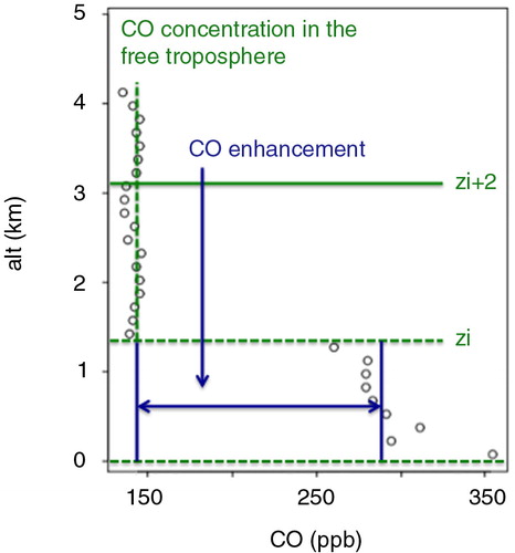
We focus on the ML as the part of the troposphere in which the contribution of local anthropogenic emissions to atmospheric mixing ratio is dominant. Conversely, above the ML, the atmosphere is mostly stably stratified, and CO mixing ratios depend mainly on long-range transport from distant emission sources. We assume that at 2 km above the top of the ML, the influence of regional surface emissions is small, and we refer to this portion of the atmosphere as free troposphere (FT). Due to the difference of transport regime in ML and FT, CO mixing ratio is usually higher in ML; the difference between mixing ratio in ML and FT is referred to as CO enhancement and is used here as a main indicator for the signal from regional surface fluxes (Fig. 1). Although due to the chaotic nature of turbulent transport and convection enhanced CO can also be found above the ML, we focus here on the much stronger enhancement within the ML.

Fig. 1 Illustration of the CO enhancement in the mixed layer (height z _i) above the CO in the free troposphere.

There are many ways to calculate the depth of the ML (z _i), but most of them are variations of the Bulk Richardson's number method or of the parcel method (Seibert et al., 2000). To establish the method of choice for the MOZAIC/IAGOS observations, we selected a sample of profiles for which it was possible to estimate the actual mixing height from the tracer's concentration profiles, and we compared the results from eight different methods with the tracer-based z _i treated as true value. The method that proved to be better in reproducing the tracer-based z _i was the parcel method with a 2 K excess temperature, which was therefore used to calculate the ML depth for each of the observed profiles.

2.2. Modelling framework

The modelling framework combines a regional transport model (STILT) with an anthropogenic emission model (EDGAR) and output from a global transport model for lateral boundary conditions (MACC). For regional atmospheric transport we use the STILT (Stochastic Time-Inverted Lagrangian Transport) model, a Lagrangian particle dispersion model. Starting from each measurement (receptor) points, STILT uses analysed wind fields from ECMWF (European Centre for Medium-range Weather Forecasts) to drive back in time for a period of 10 d ensembles of simulated particles representing air parcels of equal mass (cf. Lin et al., 2003). The model uses the back-trajectories of said particles to derive sensitivity maps of the atmospheric mixing ratio measurement to the upstream surface–atmosphere fluxes (Fig. 2, right). By matrix-multiplication with a map of surface–atmosphere fluxes (e.g. from an emission inventory), this sensitivity map returns the simulated mixing ratio corresponding to the time and location of the observation (Fig. 2, left and middle). This allows for creating simulated profiles that can be analysed in the same way as the measured ones as shown in Fig. 3, where a few exemplary profiles are given. In the following, we will refer to the Lagrangian modelling system as ‘STILT/EDGAR’.

Fig. 2 MOZAIC/IAGOS flight tracks below 4 km altitude shown on a map with CO emissions based on the EDGAR version 4.3 emissions at 10 km horizontal resolution (left), MOZAIC observation locations during 2007 in the vicinity of Frankfurt, coloured by altitude (middle), and STILT/EDGAR-derived footprint (sensitivity to upstream fluxes) for a single measurement location/time near Frankfurt airport (right).

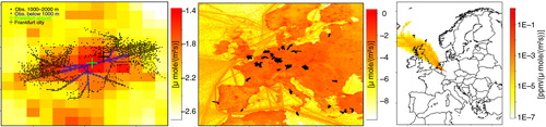
Fig. 3 Vertical profiles from MOZAIC/IAGOS observations (red), STILT/EDGAR simulations (blue) and boundary conditions from the MACC reanalysis (black) for different locations and times. Note that observations have been plotted both as continuous data (continuous red line) and averaged over 150 m intervals (red dots). The dashed lines indicate the value of z _i and z _i+2 km for the observed (red) and modelled (blue) profile, respectively.

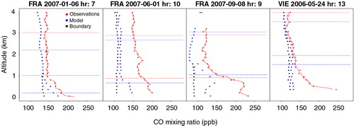
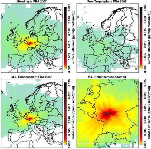
Contributions to atmospheric concentrations can be either from sources and sinks close to the receptor point or from far field advection. In modelling, the former is given from the simulated fluxes in the defined horizontal domain, whereas the latter is specified by lateral boundary conditions. STILT/EDGAR-derived profiles are obtained by summing the contributions from both within-domain fluxes and boundary conditions. Figure 3 shows profiles from observations compared with the corresponding profiles derived from STILT/EDGAR and the boundary condition derived from the MACC reanalysis (Inness et al., 2013). The difference between the latter two should give an idea of the increase in tropospheric CO mixing ratio due to the simulated fluxes close to the measurement locations. From the figure is possible to infer that there is indeed an increase from the boundary condition in the lower part of the profile, with only exception the rightmost panel in which the STILT/EDGAR profile is indistinguishable from its boundary condition. In both modelled and observed profiles, by subtracting the free tropospheric CO value from the corresponding value in the ML, the region of influence is limited to more recent emissions. A mean sensitivity map for the receptor points in the ML and FT is presented in Fig. 4, together with the sensitivity for mixed-layer enhancements computed as the difference between the above-mentioned maps for ML and FT.

Fig. 4 Illustration for STILT-derived mean surface influence for receptor points collected near Frankfurt in 2007 for the mixed layer (top left) and free troposphere (top right). The bottom panels show the enhancements from the troposphere (the difference between the former two), with different zoom.

We use STILT/EDGAR for a regional domain that covers most of Europe with a spatial resolution of 1/8 deg. latitude and 1/12 deg. longitude, corresponding to 10 km (Fig. 2, left). As lateral boundary condition for CO mixing ratios the MACC reanalysis (downloaded from www.ecmwf.int) was used.

Photochemical loss due to reaction with OH and production from CH₄ oxidation was implemented following Gerbig et al. (2003b). More detailed, the contribution to modelled CO from the advected lateral boundary condition was subject to photochemistry, but no chemical loss was included for the contribution from regional emissions, which was dominated by recent input close to the observation location with an age of typically a few hours.

For fossil fuel emissions we use EDGAR (Emission Database for Global Atmospheric Research); specifically we follow the approach taken in the COFFEE (CO₂ release and Oxygen uptake from Fossil Fuel Emission Estimate) (Steinbach et al., 2011) dataset by combining EDGARv4.3 annual global emission maps at 0.1 deg. spatial resolution for the base year 2010 provided by EDGAR (EDGARv4.2 and 4.1 are available under www.edgar.jrc.ec.europa.eu), specific for IPCC emission categories and fuel types, based on IEA (2014) fuel consumption data and EMEP/EEA (2013) emission factors. In the model, we use specific temporal factors (seasonal, weekly and daily cycles) for different emission categories, and with country and fuel type specific year-to-year changes for different fuel types at national level from the BP statistical review of World Energy 2014 (BP 2014). The basic difference to COFFEE is that here the focus is on CO rather than on CO₂ and on oxygen. This resulted in hourly resolved CO emissions, which were projected to the STILT/EDGAR EU domain. Wind fields from ECMWF have a spatial resolution of 0.25 deg. with 61 vertical levels, and a temporal resolution of 3 hours. As already mentioned in the introduction, model–data mismatch can include different aspects in both the horizontal and vertical domain, for example spatial and temporal resolution of the modelled fluxes, poorly represented convective transport in the boundary layer or biased fluxes in the emission inventory.

Even though the main focus here is on characterising error contributions from different sources, we also deem particularly important to investigate the effect of spatial resolution of simulated fluxes on model–data mismatch. As the STILT/EDGAR simulations are of course affected also by the other sources of error, we need to implement specific corrections accounting for the other dominant sources of error in order to single out the representation error. The following sections describe implemented corrections for the mismatch in observed and simulated depth of the ML, and for bias in the emission fluxes.

2.2.1. Mismatch in mixing height

The depth of the ML (z _i) is a very important variable in atmospheric modelling. In fact, in a one-dimensional model, the change in atmospheric mixing ratio of a trace gas due to underlying emissions is directly proportional to the ratio between emission flux and z _i (apart from the minor influence from the change in air density with altitude). Even assuming perfectly simulated fluxes, if the model returns a z _i that is higher (or lower) than the observed one, the simulated tracer in the ML will be too diluted (or too concentrated), leading to a net underestimate (overestimate) in the mixing ratio enhancement. Thus, tracer enhancements within the ML directly depend on the thickness of the ML itself; the same emission will lead to a larger enhancement the lower the ML depth z _i is.

STILT diagnoses z _i values from ECMWF's meteorological fields using the Bulk Richardson's number method (Lin et al., 2003). The comparisons show that in general, STILT-derived values for z _i are lower than the corresponding values diagnosed from MOZAIC/IAGOS meteorological profiles.

To account for this effect we apply a first-order correction to the simulated enhancements that adjusts modelled z _i while maintaining the column-integrated tracer amount (Kretschmer et al., 2012). Such correction is specific for each different profile and is applied only to profiles in which the simulated z _i value exceeded 225 m (the second vertical level in the MOZAIC/IAGOS profiles).

When this condition is not met in fact, the uncertainty in the observed z _i itself is expected to be too high to justify the use of a correction that adjusts the modelled value to match the observed one. Note that this situation of a simulated ML height lower than 225 m occurs predominantly at night or during winter time.

2.2.2. Flux error

Emission inventories are widely recognised as important tools for atmospheric modelling. The estimated fluxes they provide are coupled with atmospheric transport in order to simulate mixing ratios that can be compared with observations. Note that spatial distributions of population density and economic activities are often used as a proxy for emissions to downscale national emission inventories. For example, an urban population gridmap, different road maps (for the four different types of streets) and different international aviation maps (at three different heights) of Janssens-Maenhout et al. (2013) are used in this paper for gridding the CO emissions in the region around Frankfurt. Such downscaling process is not perfect and can result in biased fluxes. Differences between simulated and observed mixing ratios can then be used to quantitatively assess the emission inventories (Stein et al., 2014). In fact, as boundary condition profiles are relatively constant with height, the lion's share in the CO enhancement is accounted for by regional emissions from the emission inventories. Hence, the difference between observed and modelled enhancements reflects the difference between actual and estimated emissions.

Here we do something similar, but we take the investigation one step further. After applying the correction for ML height mismatch, we assess to which degree the emission inventory correctly simulates the emission fluxes by deriving scaling factors representing the ratio between observed and modelled CO enhancements. Secondly, we apply the obtained scaling factors to correct the model output. Using these flux-corrected CO enhancements to calculate the residuals between model and observations, we remove the flux-bias contribution to the model–data mismatch, which allows to single out the spatial representation error.

To better describe this bias, observed CO enhancements are fitted against modelled enhancements using a non-linear regression model that involves three scaling factors:1

Here sf_all is an overall scaling factor and represents the bias component in the second source of uncertainty. Conversely, sf_loc is specific for different airports (Frankfurt, London and Vienna) and thus represents spatial variations in the scaling factor while sf_month varies according to the month and allows for adjusting the seasonality of anthropogenic emissions; together, they introduce a random component in the flux error. Weighted least-squares are used to estimate the scaling factors and their uncertainties; a random error term is here indicated by ɛ.

Note that large areas with low emissions and small areas with strong emissions typically characterise fossil fuel emissions, which leads to a log-normal distribution of the enhancements. However, a least-squares optimisation of the scaling factors requires a normal distribution of the dependent variable. To account for this effect, modelled and observed enhancements were log-transformed before the optimisation of the scaling factors. As furthermore the log-transformation does not allow negative enhancements, the analysis was limited to the central 80% of the CO enhancements.

This method can be affected by biases related to the representation of photochemistry and of the lateral boundary condition. To assess this, we performed two additional STILT/EDGAR simulations: one without taking into account any photochemistry and one using a flat (zero) lateral boundary condition instead of MACC reanalysis fields for CO.

2.2.3. Representation error estimation

Spatial variations in emissions or fluxes at scales not resolved by a given tracer transport model are responsible for at least a large fraction of the spatial representation error (cf. Gerbig et al., 2003a,b). Principally such representation errors can be estimated from comparisons of simulations made at different spatial resolutions. By using a Lagrangian transport model, the grid scale at which transport is combined with the emissions is flexible. STILT has a feature that allows for transport-flux coupling at resolutions of n times the highest resolution of 10 km (the resolution of the emission inventory); here n can assume values of 1, 2, 4, 8, 16 and 32. As coarser resolved fluxes are the result of averaging over highly resolved fluxes, the effects from localised strong emission sources are reduced with decreasing spatial resolution. The representation error can thus be written in a general way as2

Here CO is the simulated CO enhancement after correction for mixing height mismatch and flux error. For each location and time, the difference between the simulated CO mixing ratio at the highest and a lower resolution can be interpreted as a single realisation of the representation error for a specific spatial scale.

Because the representation error is defined as the standard deviation of several realisations, the data need to be divided into different groups such that the representation error is not estimated as a single number, but specific for different situations. As the CO enhancements for the different airports show a strong dependence on wind direction (see results Section 3.3), we decided to group into 30° circular sectors. In addition, as wind direction determination is difficult at low wind speed, a further group ‘low wind’ was formed for wind speeds of less than 3 m/s.

As the representation error is also expected to be in some way proportional to the enhancement (in the sense that larger enhancements are associated with larger errors), we estimate a relative representation error for each airport and wind sector. For this the airport and wind sector specific data were sorted by the simulated enhancement and grouped into 10 bins of equal size. For each bin, we calculate the standard deviation of the error realisation. The random component of the relative representation error is then derived as the slope of a linear model fitting the within-bin standard deviations of the realisations against the median enhancement of the bin. The bias component was computed in a similar way, but using within-bin median instead of the standard deviation. That way each profile is associated with a relative representation error that varies between airports and wind sector. The random component corresponds to the noise in the representation error whereas the bias component represents a systematic error.

The presence of a bias component for the high-resolution STILT/EDGAR simulation after applying the correction for the flux error may seem surprising; however, it is to some degree expected: due to the log-normal distribution of the enhancements the bias correction is unbiased only for the log-transformed values, not for the enhancements themselves.

The absolute (as opposed to relative) representation error for each profile is then derived as the product between the relative representation error and the simulated CO enhancement of the considered profile.

2.2.4. Representation error validation

In order to evaluate to which degree the estimated representation error can be useful to describe and ideally predict model–data mismatch for an independent model, the representation error was compared with residuals between the MACC reanalysis and observations from MOZAIC/IAGOS.

Here we assess the dependence on wind direction and on time (month) for the random component. This was done in order to validate whether or not the representation error has any capability to describe spatial or temporal variations in model–data mismatch. The validation analysis was limited to the city of Frankfurt due to the better data coverage.

The slope of the linear regression indicates the fraction of variance and bias in the model–data mismatch that is accounted for by representation error and was derived using the Theil-Sen estimator. Such a method calculates the median of all the slopes of the lines passing through a couple of points in the graph and is therefore less sensitive to outliers. Validation results are shown only for a single spatial resolution of the STILT/EDGAR simulation (80 km). This resolution was chosen as it is closest to the MACC reanalysis horizontal resolution of 1.125 deg.

2.2.5. Contribution from different error categories

After the different sources of error (mismatch in the ML depth, bias in the emission fluxes and spatial representation error) contributing to model–data mismatch have been quantified, they can be compared to each other in order to arrive at a quantitative estimate of each source's contribution and thus to assess their relative importance.

For ML height mismatch and emission bias, the random and bias components are derived separately from mean and standard deviation respectively of the relative residuals between simulated CO enhancements before and after corrections according to eqns. (3) and (4), respectively.3 4

In assessing the contributions from the corrections, we consider the modelled values before the correction as stronger biased compared to the corresponding corrected values (in other words, corrected values are expected to be closer to the truth). The calculation was performed separately for both STILT/EDGAR and MACC. Contribution from representation error for each of the considered resolutions was derived from the mean of both random and bias component of representation error.

3. Results and discussion

3.1. Observed mixing ratios

Regular observations from MOZAIC/IAGOS allows for a thorough description of the internal structure of the troposphere. Figure 5 shows mean monthly values for CO mixing ratios collected around Frankfurt at four different heights each 1000 m. A strong seasonal cycle is present in all the investigated years, with higher mixing ratios in winter–spring and lower mixing ratios in summer–fall. CO mixing ratios around Frankfurt range between 115 and 205 ppb at 1000 m height and between 90 and 155 ppb at 4000 m. In addition, atmospheric concentration values decrease with increasing heights. It is worth pointing out that the decrease in mixing ratio between 1000 and 2000 m is much larger than the same decrease in the 2000–3000 m and 3000–4000 m step. London and Vienna have similar patterns (not shown) but different concentration ranges. In London, CO mixing ratios range from 100 to 210 ppb at 1000 m height, and from 85 to 160 ppb at 4000 m, whereas for Vienna the range is 130–220 ppb at 1000 m and 105–170 ppb at 4000 m of height.

Fig. 5 Observed CO mixing ratio for the years 2006–2011 in the lower troposphere around Frankfurt. The plots show mean monthly values at four different heights. Note that values collected at 1000 m differ strongly from values collected at higher levels. In the spring (March and April) of 2007 and 2008, higher values were collected at 2000 m and above. This is likely due to an unusually high number of spring wildfires in many European countries.

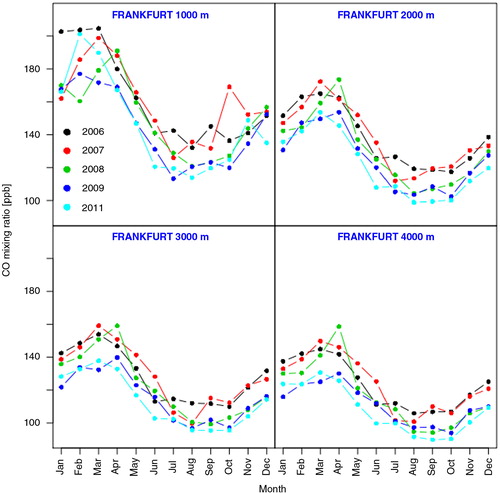
Abnormal high concentration values in the spring of years 2007 and 2008 at 3000 and 4000 m altitude are due to a much higher number of spring wildfires in many European countries in both years compared to other years. More precisely, in 2007 the affected countries were Portugal, Spain, Austria, Hungary, Germany and Czech Republic, whereas in 2008 they were Portugal, Spain, Turkey and Cyprus (Camia et al., 2009).

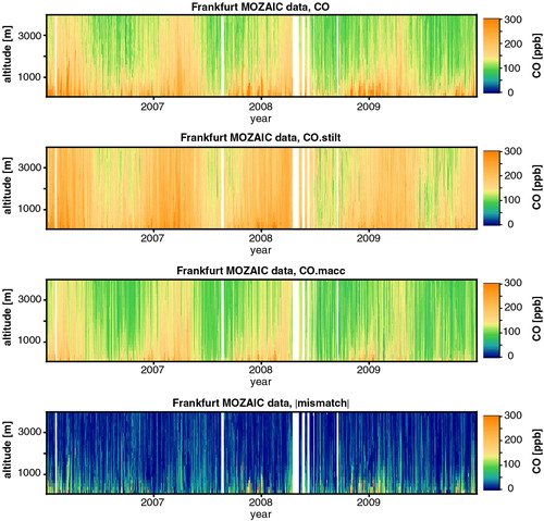
After presenting some observational results, a comparison between observation and model time series may be helpful to introduce some general remarks. Figure 6 shows an overview over 4 yr (2006–2009) of profiles between the surface and 4 km over Frankfurt. It is clear by comparing the top panel with the two middle panels that both models correctly simulate the CO seasonal cycle, although with a low-biased magnitude. The difference of observations and MACC reanalysis (bottom panel of Fig. 6) shows that larger differences are mostly located in the lower atmosphere.

Fig. 6 Observed MOZAIC/IAGOS profiles of CO near Frankfurt (first panel, on top), together with simulated profiles of CO from STILT/EDGAR coupling and MACC reanalysis (second and third panel, respectively). The bottom panel shows the absolute value of the residuals between MOZAIC/IAGOS and MACC profiles.

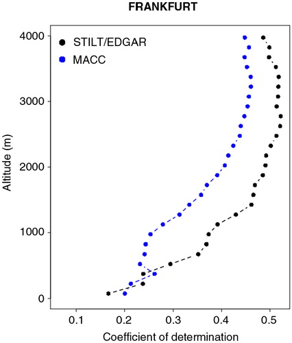
As both models returned a net underestimate of the observed mixing ratio, an attempt to evaluate their ability to simulate observations was conducted. Figure 7 shows the coefficient of determination (R ²) between modelled and observed CO mixing ratio for the different intervals of the vertical profiles derived for both STILT/EDGAR and MACC. It is evident that the models’ performance is very dependent on height and that they both perform similarly within the crucial area of the boundary layer, characterised by strong variability in the vertical transport.

Fig. 7 Coefficient of determination (R ²) between modelled and observed CO mixing ratio for both STILT/EDGAR and MACC using profiles collected around Frankfurt's airport during 2006–2011.

3.2. Corrections for mismatch in mixed layer heights

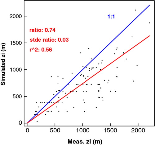
Comparisons between observed and model-derived heights of the ML (z _i) show that the modelled values are biased low for both STILT/EDGAR and MACC, although for the latter the mismatch is lower (Fig. 8 shows an example limited to 1 yr of Frankfurt data). More precisely, z _i modelled by STILT/EDGAR underestimates the observed value by 43% in Frankfurt, 53% in London and 29% in Vienna, while for MACC these values are 37% for Frankfurt, 46% for London and 17% for Vienna, respectively. From this low bias in simulated z _i one would expect a high bias in CO enhancements, corresponding to a correction that lowers the original CO enhancement.

Fig. 8 Comparison of simulated vs. observation-derived mixing heights for MOZAIC profiles near Frankfurt in 2007. The red line is drawn from the origin and through the centre of mass of the scatter plot, so its slope represents the ratio of the mean simulated and observed value.

These values translate into average corrections for the CO enhancement simulated by STILT/EDGAR of −6.8% (Frankfurt), −2.8% (London) and −9.3% (Vienna). Note that when limiting the statistics to only include those cases where modelled z _i is above 225 m (see 2.2.1), these values change to −29.9%, −15% and −29.3%, respectively. The corresponding values for the MACC reanalysis are 0.3% (Frankfurt), 6.5% (London) and 5.1% (Vienna) if all the dataset are considered, and −1%, 17.8% and 8.5% if the 225 m filter is applied.

3.3. Corrections for flux error

It is clear from Fig. 9 (left) that the CO enhancements from our STILT/EDGAR simulations are biased low. From the optimisation of the modelled fluxes using eq. (1), we found that both STILT/EDGAR simulated emissions of CO for both STILT/EDGAR and MACC reanalysis are biased low by a factor of 2–2.5 (Fig. 9, right). There is no significant difference in the scaling factors for STILT/EDGAR and MACC, as there is an overlap in the error bars of each specific correction factor. As error bars for the scaling factors of different cities also overlap, we can claim that there is no significant spatial correction. However, it is worth pointing out that a slightly significant seasonal correction is indeed present, as error bars for the scaling factors of months belonging to different seasons do not always overlap. Values for different months range from about 0.8 during summer to 1.3 during winter. The relevance of the seasonal pattern in the bias of emission models has been found to be important by Stein et al. (2014). However, their scaling factors for Europe range between 1 and 4.5 for monthly values (Table 4 from Stein et al., 2014), which corresponds to a range from 0.4 to 2.0 when separating out the overall scaling factor of 2.3, showing much stronger temporal variability than in the present study.

Fig. 9 In the left panel the comparison of simulated vs. observed mixed layer CO enhancements for Frankfurt profiles in 2007 during daytime (10:30–17:30 UTC) is shown. The red line is drawn from the origin and through the centre of mass of the scatter plot, so its slope represents the ratio of the mean simulated and observed value. The right panel shows the correction factors to compensate for a bias in STILT/EDGAR and MACC emission flux (right). Both correction factors and error bars (standard deviations) were derived using a weighted least-squares estimate of the parameters of a non-linear model.

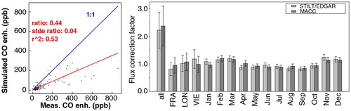
In this study, temporal emission factors for different months, days of the week and hour of the day were applied to EDGAR annual fluxes specific for both emission category and fuel. Conversely, MACCity emissions datasets used by Stein (2014) are developed on a decadal basis, with a linear interpolation applied to obtain yearly fluxes. A source-specific seasonality was then implemented.

3.4. Evaluation of simulated CO enhancement

Before quantitatively evaluating the representation error, we evaluated the statistical model with respect to ML enhancements. We are especially interested in how well the STILT/EDGAR simulations and the MACC reanalysis can reproduce the observed enhancements before and after being corrected for bias in simulated fluxes. As a high-resolution transport/flux coupling, STILT/EDGAR is expected to detect the near-field influence of emissions on the tracer enhancement.

Observed values for CO enhancements range between 30 and 130 ppb (Fig. 10) and are strongly dependent on wind direction. For all three cities, maximum values are observed when the wind blows from East, whereas minimum values are usually observed when wind blows from West. More precisely, observed enhancements over Frankfurt experience a maximum when wind direction is 45–75 deg., and a minimum when wind direction is in the interval of 255–315 deg. For London, maximum and minimum values are observed when wind direction is 75–105 and 225 deg., respectively. For Vienna data are not available for many wind sectors; among the available sectors, maximum values are collected when wind direction is 105–165 deg., whereas minimum values are collected when wind direction is 285 deg. For both Frankfurt and London, maximum enhancements correspond to situations when measurements are recorded downwind the main source region (the city centre). In addition for Frankfurt, where data coverage is better, enhancements observed under low wind conditions tend to be similar to the maximum values observed for the other sectors. This suggests that the emissions from the city centre and from the airport itself have the same potential to influence observations.

Fig. 10 Median enhancements of CO for the years 2006–2011 in the mixed layer for Frankfurt (left), London (middle) and Vienna (right), as a function of wind direction. The rightmost x-values indicated ‘low’ represent low wind speeds (<3 m/s). Observations are show in blue, STILT/EDGAR simulations in different grey tones (light for coarse, dark for high resolution), and MACC reanalysis results are shown in red. STILT/EDGAR and MACC uncorrected enhancements are shown in green and ochre, respectively.

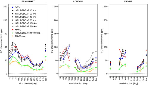
It is clear from the same plot that both STILT/EDGAR and MACC need to be corrected to avoid a severe underestimation of the observed enhancement values. As for the corrected modelled outputs, they range between 30 and 130 ppb (median over the years 2006–2011); the STILT/EDGAR simulation usually performs similarly to the MACC reanalysis in reproducing the observed enhancements in their dependence from wind direction. However, interpretation is not trivial, as the flight path depends strongly on wind direction (aircraft typically take off into the wind). It is worth noting that the enhancements derived from STILT/EDGAR for different spatial resolutions usually share a similar pattern, with a relative difference in magnitude up to 30% for Frankfurt, 50% for London and 20% for Vienna.

Note also that corrected STILT/EDGAR simulations at lower resolutions occasionally show better agreement with observations than their counterpart derived with more highly resolved fluxes. In fact, low-resolution CO enhancements tend to be reduced due to horizontal averaging of strongly localised sources; as uncorrected models systematically underestimate observed CO enhancement values, low-resolution uncorrected simulations will agree even less with observed values. However, after correction for flux error, STILT/EDGAR simulations can either overestimate or underestimate observations, which leads to the above-mentioned effect.

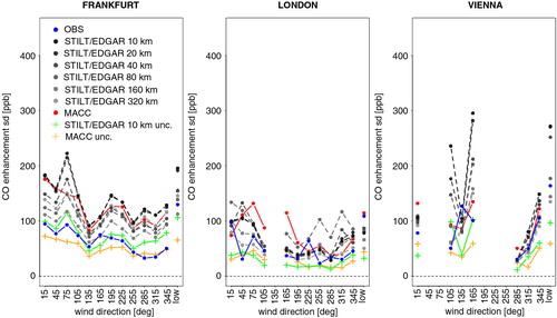
Standard deviation results are shown in Fig. 11. It is found that corrected models have a higher standard deviation than the observations whereas uncorrected models have lower standard deviations. MACC and STILT/EDGAR at highest spatial resolution (10 km) have similar standard deviations, while STILT/EDGAR's standard deviation decreases together with spatial resolution.

Fig. 11 As Fig. 10, but for the standard deviation of the enhancements of CO for the different wind sectors.

3.5. Representation error realisations

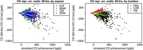
After applying the corrections for ML depth and flux error to the simulations, we plotted the realisations of representation error against the low resolution enhancements in the ML (Fig. 12). Plots were done seasonally or by location; the spatial scale of 80 km was chosen as the closest to the MACC horizontal resolution (1.125 deg.). It is clear from the plot that higher enhancements will lead to higher realisations for the representation error (see 5th–95th percentile envelopes as grey lines in Fig. 12). In addition to a larger variance, the mean of the error realisations for different simulated enhancements also shows a slight decrease for larger enhancements. In other words, the high-resolution simulations result on average in larger enhancements compared to coarser resolutions. This is related to the fact that local emissions near the IAGOS/MOZAIC observations made within the ML are strong and extend over small areas, whereas they become more diluted when using coarser resolution. Results do not show any clear dependence on the season, but slight differences can be seen for different airports.

Fig. 12 Realisations of representation error (i.e. differences between STILT simulations at different resolutions, here 10 and 160 km) for CO plotted against simulated enhancement, and colour-coded by season (left) and by airport location (right). Grey lines indicate the 5th and 95th percentile of the distribution within 10 bins of simulated enhancement; the yellow line indicates the mean.

3.6. Representation error

Both random and bias component of the representation error are highly variable with spatial resolution (Figs. 13 and 14). More precisely, representation error tends to increase with decreasing resolution even though the general dependence on wind direction is conserved.

Fig. 13 Random component of the relative representation error for CO for the years 2006–2011 in the mixed layer for Frankfurt (left), London (middle) and Vienna (right), as a function of wind direction. The rightmost x-values indicated ‘low’ represent low wind speeds (<3 m/s). STILT/EDGAR simulations are shown in different grey tones (light for coarse, dark for high resolution). Maximum relative error for Vienna at 105 degrees is up to 4.8.

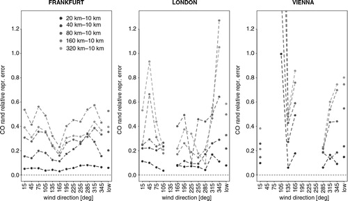
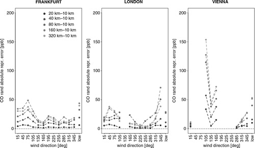
Fig. 14 As Fig. 13, but for absolute representation error.

Comparing the absolute representation error associated with the highest spatial resolution (20 km) with the representation error associated with the lowest spatial resolution (320 km), we found that such an increase can be by a factor of 4–5 for the random component, and more than 10 for the bias component. For the random component, the representation error is around 2–10% for 20 km, and with few exception increases to around 10–100% for 320 km (Fig. 13), while the range for the bias component, the representation error is from −2 to +1% at the highest resolution, and from −50 to +50% at the lowest resolution (not shown).

Most of the remarks for the relative representation error also hold for the absolute representation error, especially the strong dependence on spatial resolution. For the random component, representation error is around 2–8 ppb for 20 km and increases to around 10–50 ppb for 320 km (Fig. 14). For the bias component, values can be negative; the representation error ranges from −3 to 1 ppb at highest resolution and from −40 to 40 ppb for the lowest resolution (not shown).

Note that the random component of the representation error increases from 160 to 320 km spatial resolution for London and Vienna, but decreases for Frankfurt; this effect is probably a result of specific property of the emission pattern around the Frankfurt airport, with local emissions (which have a strong influence on the CO enhancement) being more comparable to emissions aggregated to large scale than to those aggregated to intermediate scales.

The strong dependence of representation error on both spatial resolution and wind direction indicates that coarser models are expected to have difficulties representing the small spatial scale of the emissions around strong localised sources, for example those originating in the cities. This is most likely due to the effect of horizontal dilution that such averaging has on the emissions.

3.7. Validation

In order to evaluate to which degree the representation error can be useful to describe and ideally predict model–data mismatch for an independent model, the representation error derived from STILT/EDGAR was compared with residuals between the MACC reanalysis and observations from MOZAIC/IAGOS.

Here we assess the dependence on wind direction and on time (month) in order to evaluate whether or not the representation error has any capability to describe spatial or temporal variations in model–data mismatch (Fig. 15). The analysis is limited Frankfurt due to the better data coverage.

Fig. 15 Random component for representation error of Frankfurt for different wind directions (left) and months (right), plotted against the corresponding model–data mismatch error.

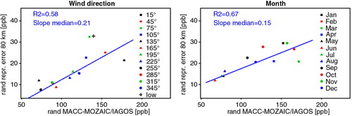
The slope of the linear regression indicates the ratio of variance in the model–data mismatch that is accounted for by representation error and was derived using the Theil-Sen estimator. Such a method calculates the median of all the slopes of the lines passing through a couple of points in the graph and is therefore less sensitive to outliers.

As mentioned in Section 2.2.4, enhancements are expected to be more or less bias free after flux error correction. Hence bias component for representation error cannot be validated and for this reason, only results for the random component are shown. In Fig. 15 it is shown that random representation error allows for describing 15–21% of the variance with good correlation coefficient returned for both wind and temporal grouping (0.58 and 0.67, respectively). Model–data mismatch ranges roughly over 60 and 180 ppb.

This result suggests that the representation error provided by STILT/EDGAR can explain a significant fraction of the random component in the model–data mismatch for MACC, and therefore, can be regarded as useful information for better understanding causes for model–data mismatch in other models.

3.8. Error contributions

After the individual errors related to mismatch in mixing height, bias in emission fluxes and spatial representation have been quantified, they can be compared to determine their relative importance. As mentioned before (Section 2.2.1), due to uncertainty in observations, we apply the correction for ML depth only when the observed z _i is higher than 225 m, which is 55% of the cases. Note that of the remaining cases, only 35% for STILT/EDGAR and 25% of MACC occur during daytime (11:00–17:00), and the rest during night-time or transition periods. This means that for almost half of the data the z _i correction factor equals one, which from the model's perspective is the same as saying that they don't need to be corrected although this is certainly not the case. To account for this effect, when we evaluate the error contributions from different categories of uncertainty, we perform our investigation only on the sub-dataset in which both the ML mismatch and flux correction are implemented.

The assessment of contribution of different error categories to model–data mismatch for the city of Frankfurt is shown in Fig. 16. Here the random and bias components are treated separately. Random and bias component for mixing layer mismatch and flux correction are here calculated according to eqns. (3) and (4), whereas both components for the spatial representation error are calculated as the mean of respective component derived in Section 2.2.3.

Fig. 16 Assessment of contribution of different error categories for the city of Frankfurt. The assessment is treated separately for random (upper tab) and bias (lower tab) component. For each component the uncertainty of the correction for mismatch in the mixing height (z _i) and bias in the emission inventories (flux) is shown for both STILT (left) and MACC (centre) models; the contribution from the spatial resolution of EDGAR fluxes to STILT/EDGAR uncertainty is shown for each of the considered resolutions (right).

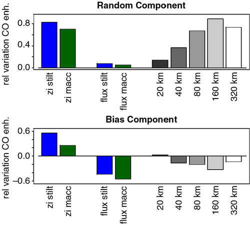
The fact that the second source of uncertainty (flux error) also has a random component is related to the fact that simulated fluxes are also corrected with a time dependent (monthly) factor. Thus, when comparing simulated CO enhancements before and after correction for flux error (overall and monthly), the standard deviation of the introduced relative differences reflects the temporally varying flux corrections.

Note the different contributions are calculated as relative errors for each category, not as the fractional contribution to the total error (i.e. the sum of the contributions is not necessarily equal to one). Random components for the mixing layer mismatch are about 83% for STILT/EDGAR simulation and 70% for MACC. The random component for flux correction is around 8% for STILT/EDGAR and 5% for MACC. Contributions from representation error range from 14 to 89% according to the considered resolution. The bias component of model–data mismatch is positive for z _i mismatch and negative for flux correction. More detailed, the relative error for ML depth is 55% for STILT/EDGAR and 26% for MACC, while for inaccuracies in simulated fluxes such values are −44% and −55%, respectively. Note that both random and bias component of the representation error increase with decreasing resolution up to 160 km, a feature observed also in the Frankfurt panel of both Figs. 13 and 14.

Further sources of error with relatively small impact are photochemistry and uncertainty due to boundary conditions. As stated in Section 2.2, the contribution to modelled CO from the advected lateral boundary condition was subject to photochemistry (reaction with OH and production from CH₄ oxidation), whereas no chemical loss was assumed for the additional CO from emissions within the domain. In fact, observations tend to be influenced the most from local sources, with the median of the time (prior to measurement) needed to account for 90% of the CO contribution from emissions is 15 hours, and with half of the CO contribution to each trajectory ensemble captured in 25 hours for 90% of the measurements. According to Protonatariou et al. (2010), CO lifetime during summer in Europe ranges from weeks to months. Using 14 d as an extreme value for CO lifetime, the amount of CO oxidised by OH in 15 hours would be to roughly 4.4% of the enhancement. We regard this as the upper limit of the uncertainty (both bias and random) introduced by neglecting photochemistry for CO from emissions within the domain.

The change in the simulated CO enhancements due to photochemistry (taken as the difference between simulations with and without photochemistry) are shown in Fig. 17 (left); the mean and standard deviation of these changes amounts to −0.7 and 2.6 ppb, respectively. Note that the photochemistry not only accounts for losses in CO, but also for CO generated by the oxidation of methane. We regard these differences as upper limit for the bias and random error resulting from imperfection in the chemistry as applied to the lateral boundary condition. Together with the uncertainty due to neglecting photochemistry for the CO emitted within the domain, the overall uncertainty in photochemistry is estimated to be on the order of 5.5% (random) and 8.9% (bias) for the CO enhancement.

Fig. 17 Absolute change in CO enhancements due to photochemistry (left) and boundary condition (right) on the whole dataset. Standard deviation of residuals is quantified as 2.6 ppb for photochemistry and 11.1 ppb for the boundary condition. Note the different scale on the x-axis of the two plots.

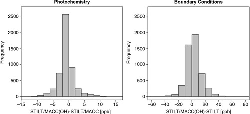
For the uncertainty due to boundary conditions we follow a similar approach by calculating residuals between STILT/EDGAR with MACC boundary condition and corresponding simulations with zero boundary condition (Fig. 17, right). The mean of the residuals is 2.9 ppb, while the standard deviation is 11.1 ppb, corresponding to 4 and 17.1% in relative terms, given average enhancements of 64 ppb. Again we regard these as upper limits for the corresponding uncertainty due to imperfect lateral boundary conditions.

Random contributions to uncertainty in the CO enhancements from both photochemistry and boundary conditions (5.5 and 4%) are comparable to those from flux correction, but much smaller than contributions from the ML depth and representation error. Note that the random error contribution from flux error is only related to the monthly variations in the correction factors, which are relatively small. As for the bias contributions from photochemistry and boundary conditions (8.9 and 17.1%), they are small compared to the other error contributions.

Other sources of error not explicitly taken into account here include uncertainty in horizontal transport and the occurrence of deep convection due to the presence of clouds. Uncertainty in simulated transport related to poor modelling of advection was thoroughly described by Lin and Gerbig (2005), where the (relatively favourable) comparison between modelled wind from the Eta Data Assimilation System (EDAS) with observation from radiosondes was used to specify uncertainty in simulated winds. Unfortunately the MOZAIC/IAGOS wind observations do not show a nearly as good agreement with the ECMWF simulated winds, most likely due to observational difficulties for airborne platforms as compared to radiosondes. We thus refrain from attempting to quantify this source of uncertainty. Uncertainty related to imperfect representation of vertical transport by deep convection is not likely to contribute strongly, as it occurs relatively infrequent.

4. Conclusion

We quantitatively described the contribution of the three major model-derived uncertainty sources: mismatch in the ML depth (related to uncertainty in the transport model), bias in the fluxes provided by the emission inventories and spatial representation error. We have shown the contribution for both random and bias component of the different model-derived error categories for both STILT/EDGAR simulations and MACC reanalysis.

Both models show similar contributions for the random component of ML depth and flux accuracy with the former clearly dominating on the latter. For both models, the bias component for ML depth has positive sign, whereas the bias component for flux accuracy has negative sign in both models. In addition, it is comparable in magnitude for STILT/EDGAR whereas in MACC the flux error is clearly more important. Contributions from spatial representation error tend to increase with degraded resolutions.

The clear dependence of representation error on both spatial resolution and wind direction shows that observations are influenced by local emissions; so high-resolution emission inventories are to be preferred for modelling applications such as inverse modelling. However, it is worth pointing out that a higher resolution model will have a direct impact on the computational effort and hence temporal and financial resources are required to carry out such simulations.

However, in this paper we have shown that spatial and temporal variation in the representation error allows for describing about one sixth to one fifth of the variance in model–data mismatch. Therefore, it is likely that information on temporal and spatial variation of representation error derived from the STILT/EDGAR simulations can be used to improve quantitative analyses when using coarse models. On the other hand, given that the spatial representation error, though significant, does not dominate the model–data mismatch, MOZAIC/IAGOS profile data can be regarded as spatially representative to a certain degree. This is good news for such a dataset, which has been collected at many locations around the globe in the vicinity of major metropolitan areas.

When considering the whole dataset, uncertainty in simulated vertical transport showed that a low bias in ML depth of 43% for EDGAR/STILT and 37% for MACC results in a reduction of CO enhancements of 6.9% and 0.3% respectively in the most representative location.

We also provided evidence that the modelled outputs for CO underestimate observations by a factor 2–2.5, suggesting a bias in the emission inventories. As most of the CO enhancements in the ML are caused by regional fluxes, rather than advected contributions from the lateral boundary, the difference between observed and modelled enhancements can be seen as the difference between actual and estimated emissions. Observations are needed to correct this underestimation, as current emission inventories are likely to perform poorly, e.g. in forecasting of regional air pollution.

Flux error is targeted in modelling to provide top-down constraint on emission inventories; however, the accuracy in top-down constrained emissions is affected by the other sources of model–data mismatch error. For example, uncertainties in ML heights and spatial representation error limit the accuracy to 30–60% (bias components in Fig. 16), thus they need to be taken into account in order to provide a more accurate top-down constraint. Note that uncertainties introduced by the (simplified) representation of photochemistry and by the choice of lateral boundary condition are rather small.

Airborne measurements are not often used for inverse (top-down) modelling of fluxes. However, given that observations from commercial airliners provide vertical profile information near major cities around the globe, and given that the emissions can be constraint by the enhancement within the boundary layer as shown here, we argue that they should be considered in inverse modelling. The method of error partitioning described in this paper will be especially important in the context of the upcoming availability of CO₂ and CH₄ profile data within IAGOS. In fact, the availability of three carbon-based tracer gases (CO, CO₂ and CH₄) will allow for multi-species inversion studies making use of a transport-flux coupling as the one described here. In this context, with different tracers that share the same transport, and that share part of their emission categories, the ability to discriminate between different sources of uncertainty will be useful. Also the use of CO as a proxy for the anthropogenic emission contribution to the CO₂ mixing ratio will be improved with the better described contributions of uncertainties to model–data mismatch.

Furthermore, as MOZAIC/IAGOS is also an important data provider for validation of satellite observations (Cal/Val), a possible future study is to perform a similar analysis aiming to assess the contributions of different sources of uncertainty contributing to satellite–airborne mismatches. A feasible option for the satellite data are the measurements from the MOPITT sensor onboard the NASA's Earth Observing System Terra spacecraft. A further alternative is represented by the IASI sensor onboard the ESA's MetOp satellite. The implementation into the IAGOS database of the information on part of the error partitioning presented in this study is envisioned in the frame of the IGAS project as a first application of our results.

Acknowledgements

The research leading to these results has received funding from the European Community's Seventh Framework Programme ([FP7/2007–2013]) under grant agreement n° 312311 (IGAS).

The authors acknowledge the strong support of the European Commission, Airbus and the Airlines (Lufthansa, Air-France, Austrian, Air Namibia, Cathay Pacific, Iberia and China Airlines so far) who carry the MOZAIC or IAGOS equipment and perform the maintenance since 1994. MOZAIC is presently funded by INSU-CNRS (France), Météo-France, Université Paul Sabatier (Toulouse, France) and Research Center Jülich (FZJ, Jülich, Germany). IAGOS has been and is additionally funded by the EU projects IAGOS-DS, IAGOS-ERI and IGAS. The MOZAIC-IAGOS database is supported by ETHER (CNES and INSU-CNRS).

Notes

This paper is part of a Special Issue on MOZAIC/IAGOS in Tellus B celebrating 20 years of an ongoing air chemistry-climate research measurement from airbus commercial aircraft operated by an international consortium of countries. More papers from this issue can be found at http://www.tellusb.net

References

- Bergamaschi P. , Hein R. , Heimann M. , Crutzen P. J . Inverse modeling of the global CO cycle: 1. Inversion of CO mixing ratios. J. Geophys. Res. 2000; 105(D2): 1909–1927.
- Bergamaschi P. , Frankenberg C. , Meirink J. F. , Krol M. , Villani M. G. , co-authors . Inverse modeling of global and regional CH4 emissions using SCIAMACHY satellite retrievals. J. Geophys. Res. 2009; 114(D22):
- Bousquet P. , Cias P. , Miller J. B. , Dlugokencky E. J. , Hauglustaine D. A. , co-authors . Contribution of anthropogenic and natural sources to atmospheric methane variability. Nature. 2006; 443: 439–443. [PubMed Abstract].
- BP (British Petroleum). Statistical Review of World Energy. 2014. Online at: http://www.bp.com/statisticalreview .
- Brioude J. , Angevine W. M. , Ahmadov R. , Kim A. W. , Evan S. , co-authors . Top-down estimate of surface flux in the Los Angeles Basin using a mesoscale inverse modeling technique: assessing anthropogenic emissions of CO, NOx and CO2 and their impacts. Atmos. Chem. Phys. 2013; 13(7): 3661–3677.
- Camia A. , San-Miguel-Ayanz J. , Oehler F. , Santos de Oliveria S. , Durrant T. , co-authors . European Commission, Joint Research Centre (JRC) – forest fires in Europe 2008. 2009
- Elguindi N. , Clark H. , Ordoñez C. , Thouret V. , Flemming J. , co-authors . Current status of the ability of the GEMS/MACC models to reproduce the tropospheric CO vertical distribution as measured by MOZAIC. Geoscientific Model Dev. 2010; 3: 501–518.
- European Commission, Joint Research Centre (JRC)/Netherlands Environmental Assessment Agency (PBL). Emission Database for Global Atmospheric Research (EDGAR), release version 4.1 and 4.2. 2011. Online at: http://edgar.jrc.ec.europa.eu .
- Gerbig C. , Lin J. C. , Wofsy S. C. , Daube B. C. , Andrews A. E. , co-authors . Toward constraining regional-scale fluxes of CO2 with atmospheric observations over a continent: 1. Observed spatial variability from airborne platforms. J. Geophys. Res. Atmos. 2003a; 108(D24):
- Gerbig C. , Lin J. C. , Wofsy S. C. , Daube B. C. , Andrews A. E. , co-authors . Toward constraining regional-scale fluxes of CO2 with atmospheric observations over a continent: 2. Analysis of COBRA data using a receptor-oriented framework. J. Geophys. Res. Atmos. 2003b; 108(D24):
- Gourdji S. M. , Mueller K. L. , Yadav V. , Huntzinger D. N. , Andrews A. E. , co-authors . North American CO2 exchange: inter-comparison of modeled estimates with results from a fine-scale atmospheric inversion. Biogeosciences. 2012; 9(1): 457–475.
- Hein R. , Crutzen P. J. , Heimann M . An inverse modeling approach to investigate the global atmospheric methane cycle. Global Biogeochem. Cy. 1997; 11(1): 43–76.
- Inness A. , Baier F. , Benedetti A. , Bouarar I. , Chabrillat S. , co-authors . The MACC reanalysis: an 8 yr data set of atmospheric composition. Atmos. Chem. Phys. 2013; 13: 4073–4109.
- Janssens-Maenhout G. , Pagliari V. , Guizzardi D. , Muntean M . Global emission inventories in the Emission Database for Global Atmospheric Research (EDGAR) – manual (I): gridding: EDGAR emissions distribution on global gridmaps. 2013. JRC Report, EUR 25785 EN. European Commission, Joint Research Centre (JRC). Luxembourg, Publications Office of the European Union..
- Kopacz M. , Jacob D. J. , Henze D. K. , Heald C. L. , Streets D. G. , co-authors . Comparison of adjoint and analytical Bayesian inversion methods for constraining Asian sources of carbon monoxide using satellite (MOPITT) measurements of CO columns. J Geophys. Res. 2009; 114(D4):
- Kretschmer R. , Gerbig C. , Karstens U. , Koch F. T . Error characterization of CO2 vertical mixing in the atmospheric transport model WRF-VPRM. Atmos. Chem. Phys. 2012; 12(5): 2441–2458.
- Lin J. C. , Gerbig C. , Wofsy S. C. , Andrews A. E. , Daube B. C. , co-authors . A near-field tool for simulating the upstream influence of atmospheric observations: the Stochastic Time-Inverted Lagrangian Transport (STILT) model. J. Geophys. Res. 2003; 108(D16):
- Lin J. C. , Gerbig C. , Daube B. C. , Wofsy S. C. , Andrews A. E. , co-authors . An empirical analysis of the spatial variability of atmospheric CO2: implications for inverse analyses and space-borne sensors. Geophys. Res. Lett. 2004; 31(23):
- Lin J. C. , Gerbig C . Accounting for the effect of transport errors on tracers inversions. Geophys. Res. Lett. 2005; 32(1):
- Machida T. , Matsueda H. , Sawa Y. , Nakagawa Y. , Hirotani K. , co-authors . Worldwide measurements of atmospheric CO2 and other trace gas species using commercial airlines. J. Atmos. Oceanic Technol. 2008; 25(10): 1744–1754. DOI: http://dx.doi.org/10.1175/2008JTECHA1082.1 .
- Marenco A. , Thouret V. , Nédélec P. , Smit H. , Helten M. , co-authors . Measurement of ozone and water vapor by Airbus in-service aircraft: the MOZAIC airborne program, an overview. J. Geophys. Res. Atmos. 1998; 103(D19): 25631–25642.
- Nassar R. , Jones D. B. A. , Kulawik S. S. , Worden J. R. , Bowman K. W. , co-authors . Inverse modelling of CO2 sources and sinks using satellite observations of CO2 from TES and surface flask measurements. Atmos. Chem. Phys. 2011; 11(12): 6029–6047.
- Nedelec P. , Cammas J. P. , Thouret V. , Athier G. , Cousin J. M. , co-authors . An improved infrared carbon monoxide analyser for routine measurements aboard commercial airbus aircraft: technical validation and first scientific results of the MOZAIC III program. Atmos. Chem. Phys. Discuss. 2003; 3(4): 3713–3744.
- Nedelec P. , Thouret V. , Brioude J. , Sauvage B. , Cammas J. P. , co-authors . Extreme CO concentrations in the upper troposphere over northeast Asia in June 2003 from the in situ MOZAIC aircraft data. Geophys. Res. Lett. 2005; 32(14):
- Petzold A. , Thouret V. , Gerbig C. , Zahn A. , Brenninkmeijer C. A. M. , co-authors . Global-scale atmosphere monitoring by in-service aircraft – current achievements and future prospects of the European Research Infrastructure IAGOS. Tellus B. 2015; 67 28452. DOI: http://dx.doi.org/10.3402/tellusb.v67.28452 .
- Protonatariou A. , Tombrou M. , Giannakopulos C. , Kostopoulou E. , Le Sager P . Study of CO surface pollution in Europe based on observations and nested-grid applications of GEOS-CHEM global chemical transport model. Tellus B. 2010; 62(4): 209–227.
- Rödenbeck C. , Houweling S. , Gloor M. , Heimann M . Time-dependent atmospheric CO2 inversions based on interannually varying tracer transport. Tellus B. 2003; 55(2): 488–497.
- Seibert P. , Beyrich F. , Gryning S. E. , Joffre S. , Rasmussen A. , co-authors . Review and intercomparison of operational methods for the determination of the mixing height. Atmos. Environ. 2000; 34(7): 1001–1027.
- Stein O. , Schultz M. G. , Bouarar I. , Clark H. , Huijnen V. , co-authors . On the wintertime low bias of Northern Hemisphere carbon monoxide found in global model simulations. Atmos. Chem. Phys. 2014; 14(17): 9295–9316.
- Steinbach J. , Gerbig C. , Rödenbeck C. , Karstens U. , Minejima C. , co-authors . The CO2 release and Oxygen uptake from Fossil Fuel Emission Estimate (COFFEE) dataset: effects from varying oxidative ratios. Atmos. Chem. Phys. 2011; 11(14): 6855–6870.
- Volz-Thomas A. , Cammas J.-P. , Brenninkmeijer C. A. , Machida T. , Cooper O. R. , co-authors . Civil aviation monitors air quality and climate. EM Magazine, Air & Waste Management Association. 2009; 16–19. October 2009.
- Zbinden R. M. , Thouret V. , Ricaud P. , Carminati F. , Cammas J. P. , co-authors . Climatology of pure tropospheric profiles and column contents of ozone and carbon monoxide using MOZAIC in the mid-northern latitudes (24° N to 50° N) from 1994 to 2009. Atmos. Chem. Phys. 2013; 13: 12363–12388.