Gas transfer velocity in the presence of wave breaking

Abstract

Wave breaking is known to cause air entrainment and enhancement of the near-surface turbulence. Thus, it intensifies the gas exchange across the air–sea interface. Based on the combination of the vertical distribution of the turbulence in the wave-affected layer and the breaking wave-energy dissipation rate in the wave-breaking layer, we proposed a composite model for the gas transfer velocity in the presence of wave breaking. The gas transfer velocity was calculated as a function of the air frictional velocity, wave age, and whitecap coverage. The model was validated by the dependences on winds and wave ages by field and laboratory measurements. The results supported the hypothesis that the large uncertainties in the traditional gas transfer velocities based on wind speed alone at moderate-to-high wind speeds can be ascribed to the neglect of the wind–wave effect, which is mainly attributed to the whitecap coverage as a function of the wind–sea Reynolds number.

• gas transfer velocity
• carbon dioxide
• wave breaking
• turbulence

1. Introduction

Carbon dioxide is of great importance because of its impact on the Earth's heat budget and climate change. To estimate the global carbon cycle, it is necessary to precisely determine the CO₂ flux between the atmosphere and oceans, which cover about 71 % of the surface of the earth. The CO₂ flux across the air–sea interface is typically estimated from the bulk formula:1 where s is the gas solubility in seawater, ΔpCO₂ is the difference in the CO₂ partial pressures of the atmosphere and ocean, and k _L is the gas transfer velocity, which is thought to be regulated by the near-surface turbulence in the case of poorly soluble gases. The turbulence intensity is generally described in terms of the turbulent dissipation rate ɛ. Lamont and Scott (1970) proposed an eddy cell model to relate the gas transfer velocity to the near-surface turbulent dissipation rate:2 where υ_w is the kinematic viscosity of water and Sc is the Schmidt number. The relation k _L −ɛ ^1/4 has been widely supported by both theoretical studies (Kitaigorodskii, 1984; Lorke and Peeters, 2006) and field measurements (Zappa et al., 2007; Tokoro et al., 2008; Vachon et al., 2010).

Since the near-surface turbulence is typically driven by wind force, the gas transfer velocity is practically parameterised as a function of U ₁₀, wind speed at a height of 10 m above sea surface (Nightingale, 2009). However, considerable differences between the different wind-speed-based gas transfer velocities have been widely documented, especially at moderate-to-high wind speeds (Wanninkhof et al., 2009). Wave breaking is supposed to be the main factor accounting for these discrepancies (Zhao et al., 2003; Woolf, 2005), because it causes air entrainment, enhances the near-surface turbulence, and thus effectively intensifies the gas exchange across the air–sea interface. To accurately parameterise the gas transfer velocity in the presence of wave breaking, it is necessary to properly determine the near-surface turbulence induced by the breaking waves.

Under the condition that the turbulent dissipation is balanced by the shear production near air–sea interface, a constant stress layer exists, which can be described by the wall layer theory (Lorke and Peeters, 2006):3 where ɛ is the dissipation rate of turbulent kinetic energy in water, u _*w is the friction velocity of water, z is the water depth, and κ=0.40 is the von Karman constant. Significant deviations from the wall layer theory could result from other dynamical processes such as breaking surface waves. Wave breaking has been found to enhance the near-surface turbulent dissipation rate by 1–2 orders of magnitude compared to the wall-layer theory (Kitaigorodskii, 1983; Agrawal et al., 1992; Anis and Moum, 1995; Drennan et al., 1996; Terray et al., 1996; Greenan et al., 2001; Soloviev and Lukas, 2003; Gemmrich and Farmer, 2004; Stips et al., 2005; Feddersen et al., 2007; Jones and Monismith, 2008; Gerbi et al., 2009). However, because of the difficulty of directly measuring the turbulence induced by breaking waves, the relation of the near-surface turbulence to the wind or wave parameters is not well understood.

Since breaking waves induce turbulence near the sea surface by dissipating the wind–wave energy, the breaking wave-energy dissipation rate provides a useful way to understand the intensity of near-surface turbulence. To estimate the breaking wave-energy dissipation rate, Hasselmann (1974) proposed a theoretical model assuming that wave breaking is weak on average and has a quasilinear spectral density. Phillips (1985) argued that in the equilibrium range, the wind input, nonlinear wave–wave interactions and dissipation are all important and derived the cubic dependence of the dissipation on the spectral density. The Phillips model is consistent with the field observations by Toba et al. (1988) and performs better in the acoustic study of wind–wave breaking (Kennedy, 1992; Felizardo and Melville, 1995) than the Hasselmann model. The breaking wave-energy dissipation rate has been related to wind and wave parameters based on the Phillips model (Hanson and Phillips, 1999; Zhao and Toba, 2001; Guan et al., 2007).

Investigating the vertical distribution of the turbulent dissipation rate, which has been widely reported to deviate from the wall layer theory in the presence of wave breaking, may also facilitate our understanding of near-surface turbulence. Craig and Banner (1994) argued that the turbulent dissipation rate should scale with z ^−3.4, which was inferred from the level 2 - 1/2 turbulence closure scheme of Mellor and Yamada (1982). Anis and Moum (1995) derived a scaling of ɛ−z ⁻³ from observations using a microscale technique. Based on observations in Lake Ontario and the results of the dimensional analysis, Terray et al. (1996) proposed a three-layer vertical distribution of turbulent dissipation rate. A wave-breaking layer (WBL) exists near the near-surface, where the turbulence is directly induced by breaking waves, and the water beneath is completely mixed (ɛ is constant). The depth of WBL (z _m) is inferred to be 0.6 H _s from the total wind input (where H _s is the significant wave height of the waves). Beneath the WBL, there exists a wave-affected layer (WAL) that turbulent dissipation is balanced by the turbulent transport from the WBL. The depth of the WAL could be extended to 6 H _s, and the vertical distribution of ɛ satisfies a scaling ɛ−z ⁻². This scaling has been supported by several studies under different environmental conditions (Drennan et al., 1996; Greenan et al., 2001; Feddersen et al., 2007; Jones and Monismith, 2008; Gerbi et al., 2009). Beneath the WAL, the turbulent transport from the WBL is negligible, and ɛ recovers to the wall layer theory.

By analysing the breaking wave-energy dissipation rate and vertical distribution of the turbulence, this study is to investigate the gas transfer velocity in the presence of wave breaking. This paper is organized as follows: Section 2 presents the observations and methods used to determine the near-surface turbulence. A composite model (CM) for the gas transfer velocity in the presence of wave breaking is proposed in Section 3. Section 4 presents the validation of the model, along with a discussion of the wave-breaking effect on the turbulence and gas transfer velocity. Finally, the conclusions are given in Section 5.

2. Near-surface turbulence

2.1. Platform observations

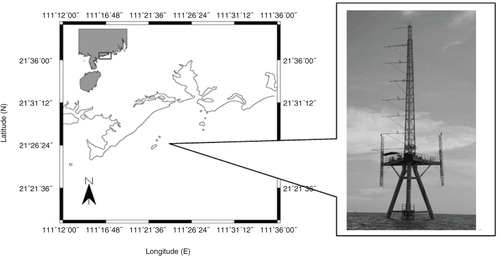
This study is part of the Flux Observation in the South China Sea (FOSCS) conducted in the coastal waters of the northern South China Sea (SCS). The objective of the programme was to understand the key processes controlling the air–sea fluxes, including the momentum, heat, and gas fluxes. Measurements were performed on a fixed platform located at (21°26′N, 111°23′E) and roughly 6.5 km southeast off the coast (Fig. 1). The height of the platform was 53 m above the sea level, and the water depth around the platform was about 15 m.

Fig. 1 Location and photograph of fixed platform.

A comprehensive system was installed to synchronously monitor the air–sea dynamics and environmental conditions. It comprised an acoustic Doppler velocimeter (ADV) to detect the turbulence in water, an eddy covariance system to measure the air–sea flux, and a Nortek acoustic wave and current (AWAC) profiler to quantify the surface wave characteristics.

The ADV was initially fixed at a water depth of 4–6 m, and the relative water depth varied with the tide in the range of 2–9 m. Because of the limited instrument memory, the ADV was set to work once an hour with the sampling frequency of 8 Hz and the duration of 8 min. The inertial dissipation method (IDM) was deployed to determine the turbulent dissipation rate.

The IDM is a well-validated method that has been routinely used to estimate the turbulence for decades. According to Kolmogorov's similarity, there exists an inertial subrange where the wavenumber spectrum of turbulent velocity has a universal form. The following equation can be used for isotropic turbulence (e.g. Orton et al., 2010):4 where k is the wavenumber, S is the wavenumber spectrum, the indices i=1 and i=2 correspond to the spectra of the horizontal and vertical velocities, respectively, and α_K is the Kolmogorov constant (0.51 when i=1 and 0.68 when i=2).

Applying Taylor's frozen hypothesis k=2πf/U to relate the wave number k to frequency f and mean advection U, eq. (4) can be converted to the frequency domain:5 where S(f) is the frequency spectrum.

Based on Fourier analysis, the frequency spectra of the horizontal (S _h) and vertical (S _v) velocities were calculated (Fig. 2), where a spectral peak occurs in the frequency range of 0.1–1 Hz. The spectral peak is more obviously for S _v that is attributed to the surface wave motion (Jones and Monismith, 2008). The spectra above the peak display the characteristics of the inertial subrange, where S(f) scales with f ^−5/3. Gerbi et al. (2009) suggested that the spectrum above wave band is elevated by unsteady advection due to the surface gravity waves. To analyse this issue, the empirical mode decomposition (Huang et al., 1998) was applied to decompose the time series of the vertical velocity into different modes. Each mode was transferred to the frequency spectrum based on Fourier analysis. As shown in Fig. 2, the frequency spectrum induced by wave motion could be identified. It can be seen that waves appear to elevate the spectrum above wave band when frequency is smaller than ~1 Hz, while the influence is negligible when frequency is greater than 1 Hz. Thus, it is reasonable to use the spectrum in the frequency range of 2–4 Hz to estimate the turbulent dissipation rate. Moreover, the spectra of the vertical velocity were adopted because they were less suffered from white noise at frequencies higher than 2 Hz. 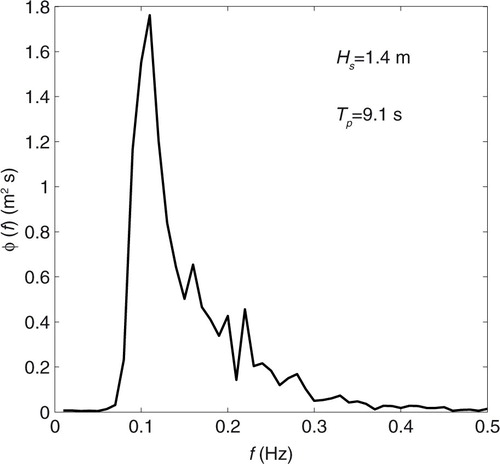Fitting the form S(f)=pf ^–5/3 for the spectrum of the vertical velocity with least-squares method, the turbulent dissipation rate could be estimated as follows:6 AWAC was deployed on the seabed near the platform. It worked once 3 h with the sampling frequency of 2 Hz and the duration of 1024 s. AWAC is deployed acoustic surface tracking (AST) to detect surface elevations and can work at a maximum depth of 60 m. It was found that AST is more precise than a pressure sensor (Pedersen and Siegel, 2008). The surface elevations were transformed into the surface wave spectrum φ(f) through Fourier analysis. An example is illustrated in Fig. 3. The significant wave height H _s, peak wave period T _p, and mean wave period T _z could be estimated from the spectrum as follows:7 An eddy covariance system was deployed at a height of 19 m above sea level to measure wind, temperature, moisture and gas fluctuations in order to determine the air–sea flux. It included an R.M. Young sonic anemometer and a LI-COR LI-7500 H₂O/CO₂ gas analyser, which both operated at the sampling frequency of 10 Hz. The wind stress could be obtained by eddy covariance method:8 where ρ _a is the air density, u is the horizontal velocity, w is the vertical velocity, the prime denoting the fluctuation of the velocity and the overbar denotes the time average. The processing procedures were performed on the raw data, including a range check and spike detection (Vickers and Mahrt, 1997) to exclude inner electronic errors and outer weather contamination such as rainfall or fog condensation. The planar fit method (Wilczak et al., 2001) was used to avoid the cross contamination of the wind velocity components induced by the inadvertent tilt of the sonic anemometer. The average timescale was determined by the multiresolution decomposition method (Vickers and Mahrt, 2003) to exclude the non-stationary mesoscale motions.

Fig. 2 Example spectra of velocity fluctuations for 8-min record, where S _v corresponds to that of vertical velocity, partitioned into wave motion and turbulence parts. S _h corresponds to that of the horizontal velocity, which was multiplied by a factor of 100 for clarity. A fit to S _v in the inertial subrange is overlaid.

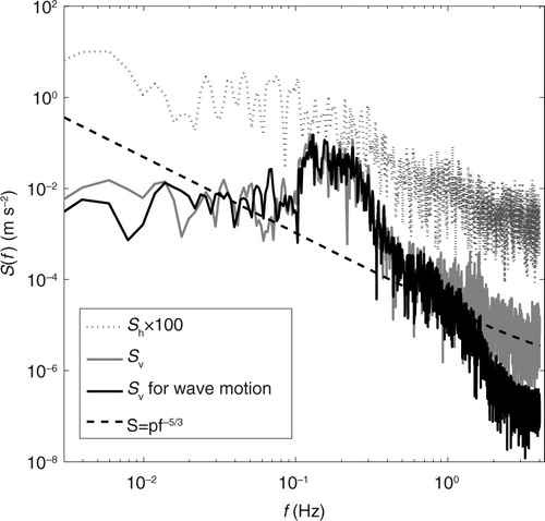
Fig. 3 Example of wave frequency spectrum derived from AWAC data.

The air frictional velocity could be derived from the wind stress: . The instantaneous horizontal wind speeds were averaged to obtain hourly mean wind speeds, which were converted to U ₁₀ using the logarithmic wind profile under neutral stability condition.

The wave-breaking events were not directly recorded by photographs during FOSCS. Many studies have shown that some parameters can be used to describe the probability of the wave breaking. Banner et al. (2000) found that the dominant breaking wave probability is strongly correlated with the significant spectral peak steepness δ_p=H _p k _p/2, where and k _p is the spectral peak wave number. It was shown that the breaking probability is zero when δ _p≤0.055 and increases quadratically when δ _p>0.055. An alternative parameter expressing wave breaking is the wind–sea Reynolds number (Toba and Koga, 1986), where υ _a is the kinematic viscosity of the air and ω _p is the spectral peak angular frequency of wind waves. Zhao and Toba (2001) showed a high correlation between whitecap coverage and R _B, and a threshold value R _B=1000 denoting the onset of wind–wave breaking (Toba et al., 1999). During FOSCS, it was found that 77 % of the observational data with δ _p>0.055, and 83 % with R _B>1000. It indicated that the wave-breaking events occurred frequently during FOSCS.

2.2. Vertical distribution of ɛ in the WAL

Terray et al. (1996) suggested that the turbulence in the WAL followed the wave-breaking scaling:9 where the exponent b=−2 and F is the wind input to the waves, which can be estimated by the growth rate formula with the directional spectrum of wind waves. Terray et al. (1996) parameterised (where is the effective wave phase speed). Because of the lack of wave direction information, we applied the routine method to parameterise (Craig and Banner, 1994). Therefore, eq. (9) could be rewritten as follows:10 The FOSCS turbulent dissipations were scaled by eq. (10), in which the coefficients α _F and b are estimated by the linear regression method. As shown in Fig. 4a, the best fit of observational data in eq. (10) is obtained with α _F =1700, b=−2.11, and the log correlation coefficient (CC) of ∣r∣=0.43. The exponent is close to −2, but α _F is several times larger than the values (90–250) as suggested by Terray et al. (1996). It should be pointed out that α _F is a function of the wave age (Wang and Huang, 2004), and Terray et al. (1996) was limited to young waves with wave age , where c _p is the phase speed of spectral peak. However, the waves around the platform are much more developed, where the wave ages range from 5 to 323. Only considering the observational data with wave age β _*<35, the best fit in eq. (10) gives rise to α _F =230, b=−2.11 and the log CC ∣r∣=0.55 (Fig. 4a). The results reveal the significant dependence of α _F on wave age.

Fig. 4 Vertical distribution of ɛ: (a) ɛH _s/u_*w versus z/H _s and (b) versus z/H _s.

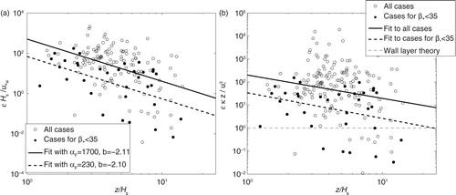
To compare the FOSCS ɛ with the wall layer theory, we scaled the normalised dissipation rate with the normalised depth z _*=z/H _s:11 where the constants a and c in eq. (11) can be determined by the linear regression method. As shown in Fig. 4b, the observational data fit in eq. (11) with a=200, c=−1.01 and the log CC ∣r∣=0.20. The observed ɛ is 2–3 orders larger than that expected from the wall layer theory within the depth, which is comparable to the wave height H _s. The enhancement is relatively small in the case of wave age β _*<35, the best fit in eq. (11) gives rise to a=34, c=−1.11 and the log CC ∣r∣=0.31.

2.3. Turbulent dissipation rate in wave-breaking layer

Assuming that the water beneath the wave-breaking patches could be fully mixed in the WBL (Weber, 2008), the near-surface turbulent dissipation rate could be derived by substituting the depth of WBL z _m into the scaling (9):12 where z _m is not well understood due to the difficulties of measurements close to the sea surface under wavy conditions. The previous studies have either scaled it with H _s (Craig and Banner, 1994; Young and Babanin, 2006; Jones and Monismith, 2008) or assigned it as constant (Gemmrich and Farmer, 1999).

Since the near-surface turbulence is greatly ascribed to wave energy dissipation through wave breaking, it could directly relate the near-surface turbulent dissipation rate to the breaking wave-energy dissipation rate:13 where R _dis is the breaking wave-energy dissipation rate and α is the proportional coefficient. This relation was supported by field measurements (Huang et al., 2012). It should be noted that z _m could be deleted by combining eqs. (12) and (13):14 In deep water, the dominant source terms of wind waves are the wind input, wave-breaking dissipation and nonlinear wave–wave interaction. The net wave growth is controlled by the wind input and wave-breaking dissipation terms because the nonlinear wave–wave interaction only causes energy exchange among wave spectral components. It has been shown that the net wave growth is one order of magnitude smaller than the wind input (Hasselmann et al., 1973; Resio, 1981; Hwang and Sletten, 2008). To the first-order approximation, we scale F with R _dis (R _dis=ρ _w F), and eq. (14) reduces to15 The breaking wave-energy dissipation rate could be estimated by the Phillips model (Hanson and Phillips, 1999):16 where δ=α/4I(p _s);ω=2πf is the radian frequency, α_* is Toba's constant ranging 0.06–0.11 and I is the directional spreading function represented by the parameter p _s ranging from 0.5 to 2 (Phillips, 1985). As a result, γδ ³ I(3p _s) is expected to be in the range of 3.7–8.0×10⁻⁴. Using the directional wave spectrum, Hanson and Phillips (1999) proposed a method to estimate the spreading function.

The JONSWAP spectra (Hasselmann et al., 1973) and wave spectra observed by buoys from the National Data Buoy Center (NDBC) were used as the input wave spectrum to the model. The JONSWAP spectra could be expressed as a function of wind speed (U ₁₀) and wave age (β=c _p/U ₁₀) (Li and Zhao, 2012). To construct the wind–wave spectrum, U ₁₀ was set as 3–25 m·s⁻¹ with an interval of 1 m·s⁻¹ and β was 0.4–1.2 with an interval of 0.1. As shown in Fig. 5, the buoys cover a wide range of wave states. Buoy 45001 is located in a closed lake; buoy 42001 in the semi-closed gulf; buoys 44014 and 46042 on the east and west coasts of America, respectively, and buoy 51028 in the open sea. As listed in Table 1, some buoys measured winds at height of 5 m. By assuming the logarithmic law of wind profile for neutral stability, these winds were converted to U ₁₀ with the drag coefficient proposed by Edson et al. (2013). Data covering the period of 2005 were chosen for analysis. Since ocean waves are generally mixed with wind waves and swell (Chen et al., 2002), the wind–wave components were separated by the spectral partitioning and wind–wave identification technique (Hanson and Phillips, 2001). In the case of wind waves, the relationship between the normalised significant wave height and period ( and ) could be well described by Toba's 3/2 power law (Toba, 1972):17 where B=0.062. The 3/2-power law was verified by Kawai et al. (1977) and Ebuchi et al. (1992). It could be seen from Fig. 6 that the derived wind–wave parameters generally agree with eq. (17), which indicates the validity of the partitioning results.

Fig. 5 Locations of buoys from National Buoy Data Center.

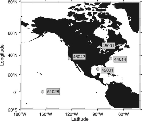
Fig. 6 The plot of non-dimensional wave height versus non-dimensional wave period.

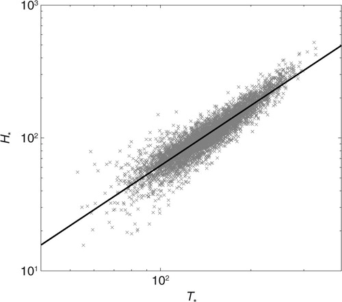
Table 1. Buoys’ information

Station	Latitude	Longitude	Depth (m)	Anemometer height (m)
44014	36.611 °N	74.842°W	95	5
45001	48.064 °N	87.777°W	261.6	5
42001	25.900 °N	89.658°W	3246	10
46042	36.785 °N	122.469°W	2098	5
51028	0.000 °N	153.913°W	4747	5

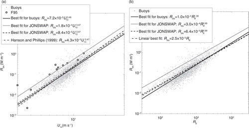
The breaking wave-energy dissipation rates were calculated using the buoys’ directional spectra with the spreading function defined by Hanson and Phillips (1999) and JONSWAP spectra with upper and lower bounds of γδ ³ I(3p _s). Attempts have been made to relate the breaking wave-energy dissipation rates to both wind and wave parameters (Guan et al., 2007; Hwang and Sletten, 2008; Kitaigorodskii, 2009). Zhao and Toba (2001), suggesting that the wind–sea Reynolds number R _B is an effective parameter describing the breaking wave characteristics in terms of whitecap coverage. With the least-squares method, the dependences of R _dis on U ₁₀ and R _B are illustrated in Fig. 7. The wind dependence of the buoys’ R _dis agrees with that of the JONSWAP spectrum with the lower bound. Both of them are generally consistent with that of Hanson and Phillips (1999), while the R _dis of the JONSWAP spectrum with the upper bound agrees well with the observational data of Felizardo and Melville (1995). A quasi-linear relationship between R _dis and R _B was illustrated with the CC (R=0.88) slightly higher than that for winds (R=0.86). Assuming that the breaking wave-energy dissipation rate is proportional to the product of the wave period and wind stress, a theoretical relation between R _dis and R _B can be derived (Fig. 7):18 Using eq. (17) with T _s=0.91T _p (Goda and Nagai, 1974; Wen et al., 1989) and the dispersion relation for deep water, the wind–sea Reynolds number could be rewritten as follows:19 Substituting eq. (18) and eq. (19) into eq. (15), the near-surface turbulence could be rewritten as follows:20 Given that ρ _w and υ _a are physical constants, the near-surface turbulent dissipation rate is a function of u _*a and β _* in the presence of wave breaking.

Fig. 7 Breaking wave-energy dissipation rates as functions of U ₁₀ (a) and R _B (b). The small circles in the figure denote the data from Felizardo and Melville (1995).

3. Model of gas-transfer velocity in the presence of wave breaking

Since wave breaking significantly enhances the turbulence beneath the sea surface, it is necessary to separate the contributions of the ‘non-breaking’ part k _NB and the ‘breaking’ part k _B to the gas exchange in the presence of wave breaking (Monahan and Spillane, 1984):21 Equation (21) could be rewritten as follows by introducing the fractional whitecap coverage W:22 where k _n is the gas-transfer velocity corresponding to the non-breaking surface, and k _w is that for the breaking surface. The latter could be obtained by substituting eq. (20) into eq. (2):23 where . It was noted that k _w depends on wind waves, which should be scaled in terms of the wave phase speed, wave height and wavelength (Fairall et al., 2000).

For the non-breaking surface, the linear dependence of the gas transfer velocity on the frictional velocity is widely supported by many studies (Deacon, 1977; Jähne et al., 1987; Lorke and Peeters, 2006). We adopt the parameterisation for a free wavy surface by Münnich and Flothmann (1975):24 Substituting eq. (23) and eq. (24) into eq. (22), a CM is proposed as follows:25 where k _L is expressed in the unit of m·s⁻¹.

It should be noted that both k _n and k _w show relatively weaker dependence on winds than that of the W proposed in the literature, such as the W−u _*a ³ proposed by Wu (1979). It is indicated that the whitecap coverage is an important parameter in characterising the gas transfer velocity. Based on the measurement of Wanninkhof et al. (1995), Zhao et al. (2003) directly related k _L to W 26 where k _L is expressed in the unit of cm·h⁻¹. Considered the bubble effect on the gas exchange, Woolf (2005) suggested that gas transfer velocity can be separated as ‘breaking’ and ‘non-breaking’ contributions:27 where k _L is expressed in the unit m·s⁻¹.

Whitecap coverage is commonly used to quantitatively describe the breaking intensity of wind waves. More than a dozen empirical models as a function of wind speed have been proposed so far. However, they exhibit great discrepancies as reported by Anguelova and Webster (2006). Recent studies indicated that the whitecap coverage is influenced by the state of the wind wave development. It has been shown that the larger whitecap coverage, the more developed wind waves at the same wind speed (Stramska and Petelski, 2003; Lafon et al., 2004; Sugihara et al., 2007; Callaghan et al., 2008; Goddijn-Murphy et al., 2011), while the existence of swell appears to suppress the whitecap coverage (Sugihara et al. 2007; Goddijn-Murphy et al., 2011). Based on comprehensive observational data, Zhao and Toba (2001) found that whitecap coverage is better correlated with the wind–sea Reynolds number R _B than the wind speed alone, and they proposed a quasi-linear relationship:28 Substituting eq. (28) into eq. (26), Zhao et al. (2003) deduced the gas transfer velocity as a function of the wind–sea Reynolds number. They suggested that the gas transfer velocity depended on not only the wind speed but also the wave age. The large uncertainties in the traditional relationship between the gas transfer velocity and wind speed could be ascribed to neglecting the effect of the wind waves. Following a similar method, Woolf (2005) and Zhao and Xie (2010) further demonstrated that the traditional gas transfer velocities are comparable to the parameterisations of eqs. (26) and (27) at different wind–wave states. Although the wave-age dependence appeared to provide a promising explanation for the large uncertainties existing in the U ₁₀-based models, it has not yet been fully validated against observations. The next section presents the validations on the W-related gas transfer velocities.

4. Validation and discussion

4.1. Model validations

Air–sea gas exchange experiments (GasEx-1998) were carried out at a significant CO₂ sink in the North Atlantic (46°6′N, 20°55′W) during June 1998 (McGillis et al., 2001). The air–sea CO₂ flux measurements were performed by the eddy covariance technique, representing one of the most successful direct covariance measurements of the air–sea CO₂ flux up to now. Air–sea CO₂ partial pressures were measured simultaneously and the gas transfer velocities were estimated from the bulk formula of eq. (1). The gas transfer velocity ranged from 0 to 120 cm·h⁻¹, and U ₁₀ ranged from 0 to 16 m·s⁻¹. Applying the least-squares method, McGillis et al. (2001) deduced a cubic dependence on wind speed of k _L:29 The wave information was not provided for GasEx-1998. Thus, we performed a numerical simulation to obtain the synchronous wave statistics through the WAVEWATCH III wave model (Appendix). These simulations indicated that the surface waves were mixed with wind waves and swell. The spectral partitioning and wind–wave identification techniques (Hanson and Phillips, 2001) were used to extract the wind–wave component. 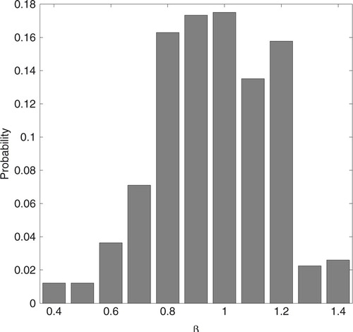To quantify the state of wind–wave development at the GasEx-1998 site, the wave age β was determined by the peak period of the wind wave and wave dispersion relation for deep water:30 As shown in Fig. 8, wind–waves approach to the fully developed stage with an average wave age of 0.98, which is generally expected for the open ocean because of the sufficiently long fetches for wave growth.

Fig. 8 Probability distribution of wave age.

Wave breaking is the most striking phenomenon under extreme wind conditions. Iwano et al. (2013) performed measurements of k _L at wind speeds of up to 70 m·s⁻¹ in a wind–wave tank. By measuring the changes of CO₂ concentration with the mass balance method, the measured gas transfer velocities ranged from 10 to 1000 cm·h⁻¹. The air frictional velocity and significant wave height were also measured, and the results are shown in their Figs. 2–7. The wave peak period could be derived from the u _*a and H _s values by Toba's 3/2 power law with T _s=0.91T _p (Goda and Nagai, 1974; Wen et al., 1989) and the dispersion relation for deep water:31 The wave ages (β) calculated from eqs. (30) and (31) ranged from 0.01 to 0.03, representing the young wave conditions expected in a wave tank due to the short wind fetch. As a result, the large differences in the wave state conditions between GasEx-1998 and the wind–wave tank provided a useful way to quantify the wave-age dependence of k _L.

Direct comparisons were performed between the observed gas transfer velocities from the two experiments and those estimated from the CM eq. (25), as well as those from eq. (26) by Zhao et al. (2003) (Z03) and from eq. (27) by Woolf (2005) (W05). In these calculations, W was estimated from the wind–sea Reynolds number by eq. (28). The results from the U ₁₀-based eq. (29) by McGillis et al. (2001) (M01) were also illustrated as a reference. For GasEx-1998, the drag coefficient formula proposed by Edson et al. (2013) was used to convert U ₁₀ to u _*a.

The comparisons are illustrated in Fig. 9. Since the upper limits of the gas transfer velocity between the field and laboratory experiments differed by almost an order of magnitude, we used a linear scale for the coordinate values in the range of 0–100 cm·h⁻¹ and a logarithmic scale in the form of 20 log₁₀ at a higher range (>100 cm·h⁻¹) for clarity. The gas transfer velocities in the field were averaged with 1 m·s⁻¹ bin of wind speed. Total 15 averaged values varying with wind speeds from 1 to 15 m·s⁻¹ are obtained. The error bars in Fig. 9 represent the standard deviation of the biases.

Fig. 9 Field (GaxEx-1998) and laboratory comparisons of k _L for (a) CM, (b) Z03, (c) W05 and (d) M01.

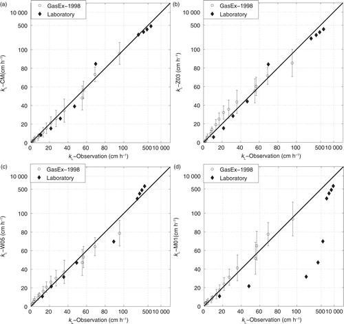
As shown in Fig. 9a, a good agreement was obtained between the observed gas transfer velocities and those from CM with B _T =0.1713 in eq. (25). A significant overestimation was found for M01 when laboratory observations are compared with field observations in the overlap wind range (0–20 m·s⁻¹). This overestimation of gas transfer velocities for laboratory observation was about 2–6 times in the range of 0–40 cm·h⁻¹. With the increasing wind speed, the overestimation of M01 became more significant up to 1–2 orders of magnitude. The large uncertainties were much improved for the three wave-age dependence models, which were generally consistent with the observations in field and laboratory experiments, although Z03 and W05 tended to slightly overestimate the gas transfer velocity of field for U ₁₀≤10 m·s⁻¹. Moreover, the uncertainty of field in terms of the standard deviation of the biases was clearly improved by CM, Z03 and W05 compared to that of M01 for U ₁₀>10 m·s⁻¹. It is clear that CM perform best over the entire wind range. Given the improved estimation from the wave-age dependence models in both the field and laboratory experiments, it is reasonable to conclude that wind waves play an important role in the gas exchange across the air–sea interface at moderate-to-high wind speeds.

A quantitative analysis was conducted in terms of the mean biases (MB), root mean square errors (RMSE) and CC, which were listed in Table 2. Compared to the M01, CM improved the RMSE by 23.8 %, while Z03 and W05 showed larger RMSE values, especially for U ₁₀≤10 m·s⁻¹. Only considering the results at moderate-to-high wind range (U ₁₀>10 m·s⁻¹), the improvement for CM was up to 30.0 %, and for Z05 and W05 was 21.8 and 19.9 %, respectively. It is evident that the best correlations between the estimation and observation were obtained by CM and W05, which both express the gas transfer velocity as the sum of the breaking and non-breaking contributions.

Table 2. Analytic statistics for gas transfer velocities estimated from different models: CM (composite model), Z03 (Zhao et al., 2003), W05 (Woolf, 2005) and M01 (McGillis et al., 2001)

	Total U 10			U 10>10 m·s^−1
	MB (cm·h^−1)	RMSE (cm·h^−1)	CC (%)	MB (cm·h^−1)	RMSE (cm·h^−1)	CC (%)
CM	0.12	6.74	94	0.15	12.11	90
Z03	6.97	10.94	91	2.67	12.92	88
W05	1.08	8.50	93	−2.29	13.12	90
M01	0.58	8.35	91	3.18	15.73	84

4.2. Discussions

4.2.1. Vertical distribution of turbulence

The breaking waves significantly enhance the near-surface turbulence, as well as the turbulence in the downward water within the WAL through turbulent diffusion. The vertical distribution of the turbulent dissipation rate in FOSCS was well consistent with Terray's scaling, which was derived from lake measurements. This scaling has also been supported by observations from nearshore shallow water (Feddersen et al., 2007) and the shallow estuarine embayment (Jones and Monismith, 2008). The consistent results implied a universal vertical distribution of the turbulent dissipation rate in WAL predicted by Terray's scaling.

The results in Section 2.2 indicated that the turbulent dissipation rate is higher with increasing wave age for a given normalised depth. Due to the large ranges of wave age, the FOSCS waves were mixed with wind waves and swell. Anis and Moum (1995) speculated that turbulence induced by the wave breaking could be transported downward by the motion of the swell, because higher values of ɛ occur deeper than the e-folding scales of the wind waves. They divided the surface mixed layer into an upper layer (1.5–5.5 m) dominated by the wind waves and a lower layer (5.5–14.5 m) dominated by the swell. Since the FOSCS results are generally within the lower layer, the higher values of dissipation are attributed to the higher vertical turbulent diffusivity induced by the swell. This issue is beyond the scope of this study because we focus on only the turbulence in the WBL.

There have been studies suggesting that Terray's scaling only holds for the H _s of wind waves in which the swell components were excluded (Greenan et al., 2001; Gerbi et al., 2009). However, the FOSCS results indicated that Terray's scaling is also valid for the H _s of mixed waves. As this may be ascribed to the ADV deployed deep enough, the swell effect could have been included.

4.2.2. Wave-age dependence

The wave-age dependence of the gas transfer velocity was well validated because the W-related models clearly improved the estimation in comparison with the results of field and laboratory experiments, and compared to the U ₁₀-based model (M01). Using the observed gas transfer velocity from the dual deliberate tracer method and wave age derived from the wave spectrum simulated by WAVEWATCHIII, Smith et al. (2011) found that the gas transfer velocity estimated from Z03 and W05 exhibited a significant overestimation and poorly correlated with the observed gas transfer velocity. They also suggested that the determination of W from the wind–sea Reynolds number using eq. (28) could be contaminated by the existing swell, as it generally dominates the spectral peak, and suppress wave breaking in opposition to wind waves (Sugihara et al., 2007; Goddijn-Murphy et al., 2011). This can be improved by the spectral peak of the wind waves separated from the wave spectrum with the 2-D wave spectrum partitioning technique. Moreover, the dual deliberate tracer method resolves the gas transfer velocity in timescale of a day (Wanninkhof et al., 2009), which may be too coarse to capture the variations with the wave state, especially at high wind speeds.

As illustrated by the CM, the wind–wave state affected gas transfer velocity through k _w, W and u _*a. The sensitivity of W to the wave state was much stronger than the effect of wave state on the drag coefficients (Woolf, 2005), and the wave-age dependence of k _w was also found to be much weaker than that of W. As a result, the wave-age dependence of k _L should be mainly attributed to the wave-age dependence of the whitecap coverage.

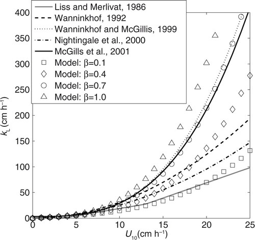
The wind and wave-age dependence of the gas transfer velocity of CM was illustrated in Fig. 10. It can be seen that the scatter of different U ₁₀-based models generally corresponds to the CM with different wave ages. As illustrated in Section 4.1, the M01 model proposed for GasEx-1998 significantly overestimated the gas transfer velocity in laboratory. This is because that wind wave during GasEx-1998 was much more developed than that in laboratory. The gas transfer velocity model (CM, Z03 and W05) including the wind–wave effect performs consistently in field and laboratory. The results indicated that the large uncertainty in the traditional U ₁₀-based models could be ascribed to neglecting the effect of the wind waves.

Fig. 10 Gas transfer velocity as function of wind speed from CM and other U ₁₀-based models.

4.2.3. Breaking and non-breaking contributions

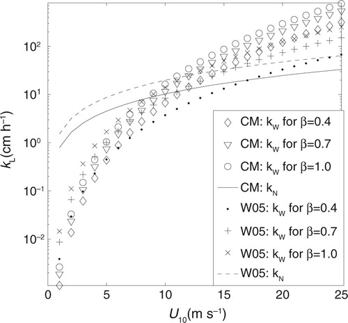
Figure 11 illustrates the breaking k _B and non-breaking k _NB contributions for CM, as well as those for W05. It can be seen that the non-breaking contribution k _NB dominated at low wind speeds (U ₁₀<6 m·s⁻¹), while the breaking contribution k _B exhibited much stronger wind dependence and dominates at high wind speeds (U ₁₀>14 m·s⁻¹). This is consistent with Hare et al. (2004) who suggested more than 80 % of the CO₂ flux at the wind speed of 14 m·s⁻¹ resulting from the breaking wave processes. The cross points of k _B and k _NB occur at moderate wind range of 8–10 m·s⁻¹, representing the transition of the dominant contribution from non-breaking to breaking. The results implied that the wind and wave-age dependence of W must be considered at moderate-to-high wind speeds, whereas the wind speed alone is accurate enough to describe the gas transfer velocity at low wind speeds. This is why the relatively small uncertainty in the traditional U ₁₀-based models at low wind speeds. The overestimation of W05 at low wind speeds could be attributed to that of k _N . The k _B of W05 exhibited weaker wind dependence than that of CM. It should be noted that the k _w for the breaking contribution is scaled by a constant 0.0024 (k _w =0.0024W) in W05, but the k _w in CM is scaled by wind and wave parameters reflecting the significantly enhanced near-surface turbulent dissipation rate beneath a breaking patches compared to that of a shear boundary layer. In this sense, the CM is more appropriate to describe the gas transfer velocity in the presence of wave breaking.

Fig. 11 Gas transfer velocity for ‘breaking’ and ‘non-breaking’ as a function of wind speed.

5. Conclusion

A CM for the gas transfer velocity was proposed by analysing the near-surface turbulence induced by wave breaking. The near-surface turbulence dissipation rate was determined by the combination of the vertical distribution of the turbulence in the WAL and the breaking wave energy dissipation rate in the WBL. It was shown that the turbulence is enhanced by 2–3 orders of magnitude in the WBL compared to that of expected from the wall-layer theory, and the vertical distribution of the turbulence in the WAL agrees with that reported by Terray et al. (1996). The breaking wave-energy dissipation rate was found to be linearly proportional to the wind–sea Reynolds number, which is directly related to the near-surface turbulence dissipation rate.

The new model for the gas transfer velocity was expressed as a function of the air frictional velocity, wave age and whitecap coverage. Based on the whitecap coverage estimated from the wind–sea Reynolds number (Zhao and Toba, 2001), the model was validated against both field and laboratory measurements for the fully developed and very young wind waves, respectively. The uncertainties in gas transfer velocities based on wind speed alone could be largely ascribed to neglecting the wind–wave effect, which is mainly represented by the whitecap coverage. The swell effect on the gas transfer velocity should be investigated in the future since it may suppress the whitecap coverage (Sugihara et al., 2007; Goddijn-Murphy et al., 2011) and prevail in the open ocean (Chen et al., 2002). Previous studies have also documented other mechanisms in the wave-breaking process on the gas exchange across the air–sea interface, such as the bubble effect (Woolf, 1997; McNeil and D'Asaro, 2007) and effect of sea spray droplets (Wanninkhof et al., 2009). It is believed that the surface area of bubbles would significantly increase the gas exchange interface. Since the coverage of bubble plume could be used as the laboratory analog of W (Asher et al., 1996), the bubble effect may enlarge the coefficient B _T in CM. The spray droplets generated by wave breaking have been recognised to effectively alter the momentum flux and heat flux through the air–sea interface (Zhao et al., 2006), but their effect on the gas transfer velocity is not well understood. Iwano et al. (2013) suggested that the volume flux of spay droplets lost through the outlet of a tank only accounted for <8 % of the total CO₂ flux, even at the highest wind speed (~70 m·s⁻¹). Thus, it is reasonable to infer that the effect of sea sprays on gas transfer can be neglected.

6. Acknowledgements

This is supported by the National Natural Science Foundation of China (Nos. 41276015 and 41076007), the Public Science and Technology Research Funds Projects of Ocean (No. 201505007), the National High Technology Research and Development Program of China (2013AA09A505), the China Postdoctoral Science Foundation (No. 2014M561972), the Research Fund for the Doctoral Program of Higher Education of China (No. 20120132110004), the Joint Project for National Oceanographic Center by the NSFC and Shandong Government (U1406401), the NSFC Innovative Group (No. 41421005) and the NSFC–Shandong Joint Fund for Marine Science Research Centers (No. U1406401).

Appendix

A.1. Wave simulation for GasEx-1998

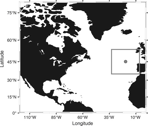
A numerical wave simulation was performed to obtain the wave statistics during the GasEx-1998 study. Since the GasEx-1998 site has a depth of ~3740 m and represents the deep water condition, version 3.14 of the third-generation spectral wave model WAVEWATCHIII was chosen, which has been successfully applied in global- and regional-scale studies in many areas, including the North Atlantic (Dodet et al., 2010). The model was run on a spatial grid of 0.25 °×0.25 ° at a longitude of 5 °–35 °W and latitude of 35 °–55 °N (Fig. 12), and the water depth was used the 1-min gridded elevations/bathymetry for the world (ETOPO2). The wave spectrum was resolved into 24 regular azimuthal direction bins and frequency bins logarithmically spaced from 0.04118 to 0.7186 at intervals of Δf/f=0.1. In order to satisfy the Courant-Friedrichs-Lewy (CFL) condition, the spatial propagation time step was set to 300 s in both the longitude and latitude directions.

Fig. 12 The domain (square) of the numerical simulation.

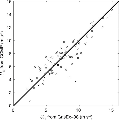
The model was forced with the cross-calibrated multi-platform (CCMP) wind field (Atlas et al., 2011), characterised by a spatial resolution of 0.25 °×0.25 ° and a temporal resolution of 6 h. The CCMP wind was derived using the variation method, and it combined several satellite wind vector measurements, including those from the advanced earth observing satellite second-generation (ADEOS-II), QuikSCAT, tropical rainfall measuring mission microwave imager (TRMM TMI), special sensor microwave imager (SSM/I) and advanced microwave scanning radiometer, while altimeter measurements were not assimilated. The comparison between the CCMP wind speed and that observed by GasEx-1998 revealed a good agreement (Fig. 13) with a CC of 0.91.

Fig. 13 Comparison of U ₁₀ values between GasEx-1998 and CCMP.

The model was run from 28 May 1998 to 20 June 1998, with standard operational default settings that included the Tolman and Chalikov (1996) source functions, and was initialised over a 5-d period to reach a stationary model output. Hourly wave directional wave spectra were derived at the GasEx-1998 site, which were used to calculate the wave statistics (such as H _s ) and determine the peak period of wind waves using the 2-D spectral partitioning technique (Hanson and Phillips, 2001).

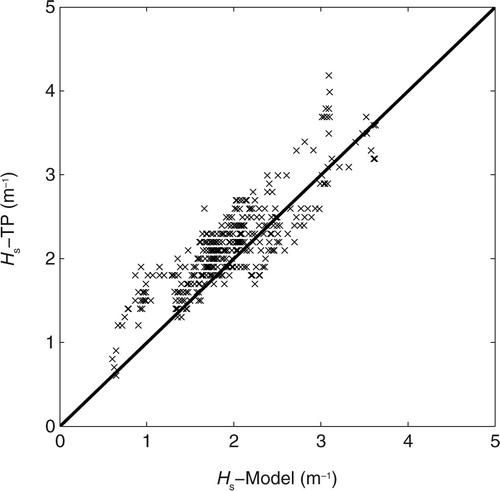
To validate the model simulation, coincident altimeter Topex/Poseidon (T/P) track measurements of H _s were used. T/P provided a 6.8-km resolution along the satellite tracks and measured H _s using both the Ku and C bands. The precision of H _s from the C band was found to be slightly better (Zhao et al., 2012). A comparison between the model H _s and that of T/P at the C band revealed a generally good agreement (Fig. 14), with a CC of 0.84.

Fig. 14 Comparison of H _s values between along-track altimeter and wave model.

References

- Agrawal Y. C. , Terray E. A. , Donelan M. A. , Hwang P. A. , Williams A. J. , co-authors . Enhanced dissipation of kinetic energy beneath surface waves. Nature. 1992; 359: 219–220.
- Anguelova M. D., Webster F. Whitecap coverage from satellite measurements: a first step toward modeling the variability of oceanic whitecaps. J. Geophys. Res. 2006; 111: C03017. DOI: http://dx.doi.org/10.1029/2005JC003158.
- Anis A. , Moum J. N . Surface wave–turbulence interactions. Scaling ɛ(z) near the sea surface. J. Phys. Oceanogr. 1995; 25: 2025–2045.
- Asher W. E. , Karle L. M. , Higgins B. J. , Farley P. J. , Monahan E. C. , co-authors . The influence of bubble plumes on air-seawater gas transfer velocities. J. Geophys. Res. 1996; 101: 12027–12041.
- Atlas R., Hoffman R. N., Ardizzone J., Leidner S. M., Jusem J. C., co-authors. A cross-calibrated, multiplatform ocean surface wind velocity product for meteorological and oceanographic applications. Bull. Amer. Meteor. Soc. 2011; 92: 157–174.
- Banner M. L. , Babanin A. V. , Young I. R . Breaking probability for dominant waves on the sea surface. J. Phys. Oceanogr. 2000; 30: 3145–3160.
- Callaghan A. H., Deane G. B., Stokes M. D. Observed physical and environmental causes of scatter in whitecap coverage values in a fetch-limited coastal zone. J. Geophys. Res. 2008; 113: C05022. DOI: http://dx.doi.org/10.1029/2007JC004453, 2008..
- Chen G. , Chapron B. , Ezraty R. , Vandemark D . A global view of swell and wind sea climate in the ocean by satellite altimeter and scatterometer. J. Atmos. Oceanic Technol. 2002; 19: 1849–1859.
- Craig P. D. , Banner M. L . Modeling wave-enhanced turbulence in the ocean surface layer. J. Phys. Oceanogr. 1994; 24: 2546–2559.
- Deacon E. L . Gas transfer to and across an air–water interface. Tellus A. 1977; 29: 363–374.
- Dodet G. , Bertin X. , Taborda R . Wave climate variability in the North–East Atlantic Ocean over the last six decades. Ocean Model. 2010; 31: 120–131.
- Drennan W. M. , Donelan M. A. , Terray E. A. , Katsaros K. B . Oceanic turbulence dissipation measurements in SWADE. J. Phys. Oceanogr. 1996; 26: 808–815.
- Ebuchi N. , Toba Y. , Kawamura H . Statistical study on the local equilibrium between wind and wind waves by using data from ocean data buoy stations. J. Oceanogr. Soc. Japan. 1992; 48: 77–92.
- Edson J. B. , Jampana V. , Weller R. A. , Bigorre S. P. , Plueddemann A. J. , co-authors . On the exchange of momentum over the open ocean. J. Phys. Oceanogr. 2013; 43: 1589–1610.
- Fairall C. W. , Hare J. E. , Edson J. B. , McGillis W . Parameterization and micro-meteorological measurements of air–sea gas transfer. Boundary Layer Meteorol. 2000; 96: 63–105.
- Feddersen F. , Trowbridge J. H. , Williams A. J . Vertical structure of dissipation in the nearshore. J. Phys. Oceanogr. 2007; 37: 1764–1777.
- Felizardo F. C. , Melville W. K . Correlations between ambient noise and the ocean surface wave field. J. Phys. Oceanogr. 1995; 25: 513–532.
- Gemmrich J. R. , Farmer D. M . Near-surface turbulence and thermal structure in a wind-driven sea. J. Phys. Oceanogr. 1999; 29: 480–499.
- Gemmrich J. R. , Farmer D. M . Near-surface turbulence in the presence of breaking waves. J. Phys. Oceanogr. 2004; 34: 1067–1086.
- Gerbi G. P. , Trowbridge J. H. , Terray E. A. , Plueddemann A. J. , Kukulka T . Observations of turbulence in the ocean surface boundary layer: energetics and transport. J. Phys. Oceanogr. 2009; 39: 1077–1096.
- Goda Y. , Nagai K . Investigation of the statistical properties of sea waves with fields and simulated data (in Japanese). Rep. Port Harbor Res. Inst. 1974; 13: 3–37.
- Goddijn-Murphy L. , Woolf D. K. , Callaghan A. H . Parameterizations and algorithms for oceanic whitecap coverage. J. Phys. Oceanogr. 2011; 41: 742–756.
- Greenan B. J. W. , Oakey N. S. , Dobson F. W . Estimates of dissipation in the ocean mixed layer using a quasi-horizontal microstructure profiler. J. Phys. Oceanogr. 2001; 31: 992–1004.
- Guan C., Hu W., Sun J., Li R. The whitecap coverage model from breaking dissipation parametrizations of wind waves. J. Geophys. Res. 2007; 112: C05031. DOI: http://dx.doi.org/10.1029/2006JC003714, 2007.
- Hanson J. L. , Phillips O. M . Wind sea growth and dissipation in the open ocean. J. Phys. Oceanogr. 1999; 29: 1633–1648.
- Hanson J. L. , Phillips O. M . Automated analysis of ocean surface directional wave spectra. J. Atmos. Oceanic Technol. 2001; 18: 277–293.
- Hare J. E., Fairall C. W., McGillis W. R., Edson J. B., Ward B., co-authors. Evaluation of the National Oceanic and Atmospheric Administration/Coupled-Ocean Atmospheric Response Experiment (NOAA/COARE) air–sea gas transfer parameterization using GasEx data. J. Geophys. Res. 2004; 109(C8): C08S11. DOI: http://dx.doi.org/10.1029/2003JC001831.
- Hasselmann K . On the spectral dissipation of ocean waves due to whitecapping. Boundary-Layer Meteorol. 1974; 126: 107–127.
- Hasselmann K. , Barnett T. P. , Bouws E. , Carlson H. , Cartwright D. E. , co-authors . Measurements of wind–wave growth and swell decay during the Joint North Sea Wave Project (JONSWAP). Ergänzung zur Deut. Hydrogr. Z. 1973; 8: 1–95.
- Huang N. E. , Shen Z. , Long S. R. , Wu M. L. , Shih H. H. , co-authors . The empirical mode decomposition and the Hilbert spectrum for nonlinear and non-stationary time series analysis. Proc. R. Soc. Lond. A. 1998; 454(1971): 903–995.
- Huang Z., Lenain L., Melville W. K., Middleton J. H., Reineman B., co-authors. Dissipation of wave energy and turbulence in a shallow coral reef lagoon. J. Geophys. Res. 2012; 117: C03015. DOI: http://dx.doi.org/10.1029/2011JC007202.
- Hwang P. A., Sletten M. A. Energy dissipation of wind-generated waves and whitecap coverage. J. Geophys. Res. 2008; 113: C02012. DOI: http://dx.doi.org/10.1029/2007JC004277.
- Iwano K. , Takagaki N. , Kurose R. , Komori S . Mass transfer velocity across the breaking air–water interface at extremely high wind speeds. Tellus B. 2013; 65: 1–8.
- Jähne B. , Münnich K. O. , Dutzi R. B. A. , Huber W. , Libner P . On the parameters influencing air–water gas exchange. J. Geophys. Res. 1987; 92: 1937–1949.
- Jones N. L. , Monismith S. G . The influence of whitecapping waves on the vertical structure of turbulence in a shallow estuarine embayment. J. Phys. Oceanogr. 2008; 38: 1563–1580.
- Kawai S. , Okada K. , Toba Y . Field data support of three seconds power law and the spectral form for growing wind waves. J. Oceanogr. Soc. Japan. 1977; 33: 137–150.
- Kennedy R. M . Sea surface dipole sound source dependence on wave-breaking variables. J. Acoust. Soc. Amer. 1992; 91: 1974–1982.
- Kitaigorodskii S. A . On the theory of the equilibrium range in the spectrum of wind-generated gravity waves. J. Phys. Oceanogr. 1983; 13: 816–827.
- Kitaigorodskii S. A . On the Fluid Dynamical Theory of Turbulent Gas Transfer Across an Air-Sea Interface in the Presence of Breaking Wind-Waves. J. Phys. Oceanogr. 1984; 14: 960–972.
- Kitaigorodskii S. A . Determining the influence of wind–wave breaking on the dissipation of the turbulent kinetic energy in the upper ocean and on the dependence of the turbulent kinetic energy on the stage of wind–wave development. Izv. Atmos. Oceanic Phys. 2009; 45: 372–379.
- Lafon C. , Piazzola J. , Forget P. , Le Calve O. , Despiau S . Analysis of the variations of the whitecap fraction as measured in a coastal zone. Boundary-Layer Meteorol. 2004; 111: 339–360.
- Lamont J. C. , Scott D. S . An eddy cell model of mass transfer into the surface of a turbulent liquid. AIChE J. 1970; 16: 513–519.
- Li S. , Zhao D . Comparison of spectral partitioning techniques for wind wave and swell. Mar. Sci. Bull. 2012; 14: 24–36.
- Lorke A. , Peeters F . Toward a unified scaling relation for interfacial fluxes. J. Phys. Oceanogr. 2006; 36: 955–961.
- McGillis W. R. , Edson J. B. , Hare J. E. , Fairall C. W . Direct covariance air–sea CO2 fluxes. J. Geophys. Res. 2001; 106: 16729–16745.
- McNeil C. , D'Asaro E . Parameterization of air–sea gas fluxes at extreme wind speeds. J. Mar. Syst. 2007; 66: 110–121.
- Mellor G. L. , Yamada T . Development of a turbulence closure model for geophysical fluid problems. Rev. Geophys. 1982; 20: 851–875.
- Monahan E. C. , Spillane M. C . Brutsaert W. , Jirka G. H . The role of oceanic whitecaps in air–sea gas exchange. Gas Transfer at Water Surfaces. 1984; Springer, Netherlands. 495–504.
- Münnich K. O. , Flothmann D . Gas exchange in relation to other air–sea interaction phenomena. Paper presented at SCOR Workshop on Air–Sea Interaction Phenomena. 1975; FL: Miami.
- Nightingale P. D . Air–sea gas exchange. Surface ocean-lower atmosphere processes. 2009; 187: 69–97.
- Orton P., Zappa C. J., McGillis W. R. Tidal and atmospheric influences on near surface turbulence in an estuary. J. Geophys. Res. 2010; 115: C12029.
- Pedersen T. , Siegel E . Wave Measurements from Subsurface Buoys. In: Current Measurement Technology, 2008. CMTC 2008. IEEE/OES 9th Working Conference on. 2008; Charlston, SC: IEEE. 224–233.
- Phillips O. M . Spectral and statistical properties of the equilibrium range in wind-generated gravity waves. J. Fluid Mech. 1985; 156: 505–531.
- Resio D. T . The estimation of wind-wave generation in a discrete spectral model. J. Phys. Oceanogr. 1981; 11: 510–525.
- Smith M. J. , Ho D. T. , Law C. S. , McGregor J. , Popinet S. , co-authors . Uncertainties in gas exchange parameterization during the SAGE dual-tracer experiment. Deep Sea Res. Part II Top. Stud. Oceanogr. 2011; 58: 869–881.
- Soloviev A. , Lukas R . Observation of wave-enhanced turbulence in the near-surface layer of the ocean during TOGA COARE. Deep Sea Res. Part I Oceanogr. Res. Pap. 2003; 50: 371–395.
- Stips A. , Burchard H. , Bolding K. , Prandke H. , Simon A. , co-authors . Measurement and simulation of viscous dissipation in the wave affected surface layer. Deep Sea Res. Part II Top. Stud. Oceanogr. 2005; 52: 1133–1155.
- Stramska M., Petelski T. Observations of oceanic whitecaps in the north polar waters of the Atlantic. J. Geophys. Res. 2003; 108(C3): 3086.
- Sugihara Y. , Tsumori H. , Ohga T. , Yoshioka H. , Serizawa S . Variation of whitecap coverage with wave-field conditions. J. Mar. Syst. 2007; 66: 47–60.
- Terray E. A. , Donelan M. A. , Agrawal Y. C. , Drennan W. M. , Kahma K. K. , co-authors . Estimates of kinetic energy dissipation under breaking waves. J. Phys. Oceanogr. 1996; 26: 792–807.
- Toba Y . Local balance in the air–sea boundary processes. J. Oceanogr. 1972; 28: 109–120.
- Toba Y. , Kizu S. , Ebuchi N . On-board quantitative wind–wave observations using a stop watch. Prel. Rep. of The Hakuho Maru Cruise KH-88-2 (OMLET Cruise). 1988; Tokyo: Ocean Research Institute, University of Tokyo. 35–44.
- Toba Y. , Koga M . Monahan E. C. , Mac Niocaill G . A parameter describing overall conditions of wave breaking, whitecapping, sea-spray production and wind stress. Oceanic Whitecaps. 1986; Springer Netherlands, : Reidel Publishing Company. 37–47.
- Toba Y. , Suzuki Y. , Iida N . Banner M. L . Study on global distribution with seasonal variation of the whitecap coverage and sea-salt aerosol production on the sea surface. The Wind-Driven Air-Sea Interface. 1999; Sydney, Australia,: School of Mathematics, The University of New South Wales. 355–356.
- Tokoro T., Kayanne H., Watanabe A., Nadaoka K., Tamura H., co-authors. High gas-transfer velocity in coastal regions with high energy-dissipation rates. J. Geophys. Res. 2008; 113: C11006.
- Tolman H. L. , Chalikov D. V . Source terms in a third-generation wind wave model. J. Phys. Oceanogr. 1996; 26: 2497–2518.
- Vachon D. , Prairie Y. T. , Cole J. J . The relationship between near-surface turbulence and gas transfer velocity in freshwater systems and its implications for floating chamber measurements of gas exchange. Limnol. Oceanogr. 2010; 55: 1723–1732.
- Vickers D. , Mahrt L . Quality control and flux sampling problems for tower and aircraft data. J. Atmos. Oceanic Technol. 1997; 14: 512–526.
- Vickers D. , Mahrt L . The cospectral gap and turbulent flux calculations. J. Atmos. Oceanic Technol. 2003; 20: 660–672.
- Wang W. , Huang R. X . Wind energy input to the surface waves. J. Phys. Oceanogr. 2004; 34: 1276–1280.
- Wanninkhof R. , Asher W. E. , Ho D. T. , Sweeney C. , McGillis W. R . Advances in quantifying air–sea gas exchange and environmental forcing*. Annu. Rev. Mar. Sci. 2009; 1: 213–244.
- Wanninkhof R. , Asher W. , Monahan E . Jähne B. , Monahan E . The influence of bubbles on air–water gas exchange: Results from gas transfer experiments during WABEX-93. Air–water Gas Transfer. 1995; Hanau, Germany: AEON Verlag. 239–254.
- Weber J. E. H. A note on mixing due to surface wave breaking. J. Geophys. Res. 2008; 113: C11009.
- Wen S. , Zhang D. , Guo P. , Chen B . Parameters in wind wave frequency spectra and their bearing on spectrum forms and growth. Acta Oceanol. Sin. 1989; 8(1): 15–39.
- Wilczak J. , Oncley S. , Stage S . Sonic anemometer tilt correction algorithms. Boundary-Layer Meteorol. 2005; 99: 127–150.
- Woolf D. K . Liss P. S. , Duce R. A . Bubbles and their role in gas exchange. The Sea Surface Microlayer and Global Change. 1997; Cambridge, Gran Bretaña,: Cambridge University Press. 173–205.
- Woolf D. K . Parametrization of gas transfer velocities and sea-state-dependent wave breaking. Tellus B. 2005; 57: 87–94.
- Wu J . Oceanic whitecaps and sea state. J. Phys. Oceanogr. 1979; 9: 1064–1068.
- Young I. R. , Babanin A. V . Spectral distribution of energy dissipation of wind-generated waves due to dominant wave breaking. J. Phys. Oceanogr. 2006; 36: 376–394.
- Zappa C. J., McGillis W. R., Raymond P. A., Edson J. B., Hintsa E. J., co-authors. Environmental turbulent mixing controls on air–water gas exchange in marine and aquatic systems. Geophys. Res. Lett. 2007; 34: L10601.
- Zhao D. , Li S. , Song C . The comparison of altimeter retrieval algorithms of the wind speed and the wave period. Acta Oceanol. Sin. 2012; 31: 1–9.
- Zhao D. , Toba Y . Dependence of whitecap coverage on wind and wind–wave properties. J. Oceanogr. 2001; 57: 603–616.
- Zhao D., Toba Y., Sugioka K., Komori S. New sea spray generation function for spume droplets. J. Geophys. Res. 2006; 111: C02007. DOI: http://dx.doi.org/10.1029/2005JC002960.
- Zhao D. , Toba Y. , Suzuki Y. , Komori S . Effect of wind waves on air–sea gas exchange: proposal of an overall CO2 transfer velocity formula as a function of breaking-wave parameter. Tellus B. 2003; 55: 478–487.
- Zhao D. , Xie L . A Practical bi-parameter formula of gas transfer velocity depending on wave states. J. Oceanogr. 2010; 66: 663–671.