The radiative impact of Nordic anthropogenic black carbon

Abstract

This study presents an assessment of the impact of black carbon (BC) regional emissions of four Nordic countries (Denmark, Finland, Norway and Sweden – denoted henceforth as DFNS). The surface concentrations, radiative forcing and BC-in-snow forcing were calculated using ECHAM-HAMMOZ global aerosol-climate model and, where possible, evaluated with field observations. We found that the model is reproducing the BC surface concentrations for most of the measurement sites considered within 1–2 standard deviations, with only few exceptions. The radiative forcing (top of the atmosphere, short-wave, clear and total sky) of BC emitted in DFNS on regional (Nordic and Arctic area separately) and global levels was calculated by removing the anthropogenic emissions from DFNS. The total values for clear sky for the three regions are 16.2±1.4, 2.9±0.28 and 0.04±0.022 mW/m², respectively. The presence of clouds enhanced the BC radiative forcing. The forcing caused by BC deposited on snow is roughly equal to the direct radiative forcing of airborne BC (17.3±3.34 mW/m² over DFNS, 4.2±0.77 mW/m² over the Arctic and 0.042±0.012 mW/m² globally).

• black carbon
• global model
• radiative forcing

1. Introduction

Black carbon (BC) is an important aerosol in the atmosphere, with significant influences on regional and global climate due to its direct, semi-direct and indirect effects. For instance, BC absorbs and scatters radiation, resulting in warming the atmosphere and reducing the amount of solar radiation reaching the surface of Earth, affects cloud formation and cloud properties, and contributes to the accelerated melting of snow and ice in the poles and glaciers via the reduction in snow albedo (Hansen and Nazarenko, 2004; Jacobson, 2004; Koch and Del Genio, 2010; Bond et al., 2013; Lee et al., 2013). In addition, BC's diverse chemical properties ensure its association with a broad range of adverse health effects, including respiratory and cardiovascular effects as well as premature death (Janssen et al., 2011; US EPA, 2012).

Due to its relatively short life time in the atmosphere (days to weeks), BC mostly impacts the regional climate, being spatially and temporally linked to the emission sources, introducing spatial gradients in solar heating of the atmosphere and surface (Textor et al., 2006). The resulting changes in surface temperature can potentially perturb clouds and precipitation causing an alteration in water availability which, consequently, induces a sharper change in the regional rather than global climate. In addition, some regions of the world are more prone to be affected by BC forcing, either due to transport and deposition (e.g. the Arctic) (Bond et al., 2013), or due to high levels of pollution (e.g. India, China) (Wang et al., 2014). Global averages of BC forcing eclipse much of the regional variability of BC concentrations and its impact, and therefore each region of interest has to be considered individually.

In contrast to global radiative forcing, there are only few studies that have addressed the regional BC direct radiative forcing. The greater part of the studies concentrates on one of the most sensitive (to BC) regions of the globe, the Arctic (Wang et al., 2011; Flanner, 2013; Sand et al., 2013a, b; Jiao et al., 2014), while few others consider areas of a more local interest. For instance, Bahadur et al. (2011) provide a comprehensive picture of atmospheric spatial and temporal BC trends over California using observations recorded by the Interagency Monitoring of Protected Visual Environments (IMPROVE) monitoring network for 20 yr. The 50 % decrease in annual average BC concentrations from 1998 to 2008 is attributed to the reduction in diesel emissions, also of about 50 %. Mahmood and Li (2014), using the Geophysical Fluid Dynamics Laboratory (GFDL) AM2.1 general circulation model, studied the remote impact of South Asian BC aerosol on East Asian summer monsoon. The South Asian BC induced changes of about 5–10 % of the observed climatological rainfalls in East Asia. Kopacz et al. (2011) used the Goddard Earth Observation System (GEOS)-Chem model to identify the origin of the BC arriving at the Himalayas and Tibetan Plateau. The authors calculated BC direct and snow-albedo radiative forcing and provided a detailed map of the location of emissions that directly contribute to BC concentrations at the receiving locations. Hienola et al. (2013) estimated BC concentrations and deposition in Finland using the regional aerosol-climate model REgional MOdel-Hamburg Aerosol Model (REMO-HAM). Reddy and Boucher (2007), using the LMD (Laboratoire de Météorologic Dynamique) global climate model, estimated the contribution of different regions to global BC atmospheric burden and direct radiative forcing. They found that East and South Asia together contribute more than 50 % of the global surface, atmospheric, and top-of-atmosphere direct radiative forcing by BC, while Europe is the largest contributor (63 %) to BC deposition at high latitudes.

Because a large fraction of atmospheric BC concentrations is due to anthropogenic activities and because of its short atmospheric lifetime, BC represents a low-hanging fruit for rapidly slowing down the global warming through BC emission reduction. Although BC emission cuts will not solve the long-term global climate problem, they would however curb short-term climate change and reduce the impacts on vulnerable regions like the Arctic, diminish the air pollution and improve public health. The four Nordic countries (in this study we refer to Denmark, Finland, Norway and Sweden – denoted henceforth as DFNS) addressed these environmental issues by releasing a series of reports concerning methods of estimating BC emissions at national level, identifying new and existing measures to reduce BC emissions and recommendations for further immediate actions (Hansson et al., 2011; Winther and Nielsen, 2011; Aasestad, 2013; Forsberg et al., 2014). These reports, together with the DFNS countries active participation in Arctic Council, Nordic Council of Ministeries and the Climate and Clean Air Coalition, represent the starting point of this study.

The main objective of this study is to assess the radiative impact of anthropogenic BC emitted in DFNS, mainly by means of modelling studies, using the global aerosol–climate model ECHAM-HAMMOZ. The climate impact is quantified by determining the direct radiative forcing and estimating the BC-in-snow forcing of BC aerosols for DFNS, the Arctic and globally. Also included in this study is the task of evaluating the model using observational data existing in our region of interest.

2. BC emission studies in DFNS countries

Despite the rapidly increasing amount of scientific literature on BC, there is a need for a more exhaustive evaluation of both the magnitude of particular global and regional climate effects caused by BC and the impact of emissions mixtures from different source categories. To accelerate the efforts to understand the role of BC on climate change, all of the DFNS countries conducted studies on BC emissions including inventories of the major sources of BC and the identification of the approaches to reduce BC emissions (Hansson et al., 2011; Winther and Nielsen, 2011; Aasestad, 2013; Forsberg et al., 2014).

In order to obtain BC emission estimates, two different methods have been used: either from specific emission factors for different fuels used in various sectors [based on, for example, Kupiainen and Klimont (2007); Junker and Liousse (2008)] or – a more common method – based on PM_2.5 or PM₁₀ emission inventories with estimated BC fractions of PM emitted obtained from literature (Streets et al., 2001; Bond et al., 2004; Kupiainen and Klimont, 2004).

According to the authors, the heating in households represents the main BC source and contributed to about a quarter of total BC emissions in 2011. While BC emissions from the domestic sector have increased in all four countries, the road traffic emissions have decreased due to more energy efficient vehicles and introduction of stricter exhaust emission requirements, despite growth of more than 50 % in traffic since 1990.

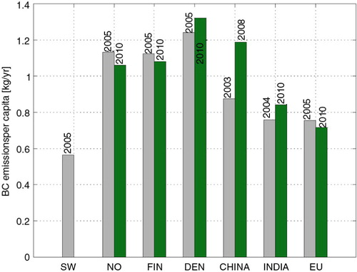
As stated in the above-mentioned reports, the total emissions of BC in DFNS have stabilised since the year 2000. Progressive introduction of diesel particle filters will reduce fine particulate matter PM_2.5 (hence BC calculated as a special fraction of PM_2.5) emissions from mobile sources by about two-thirds by 2025 compared to 2005 (Amann et al., 2014). The extent of the decrease in other sectors will depend on the rate at which control strategies are adopted. In DFNS, the residential combustion is by far the greatest target area for reduction but may also be the most difficult sector to address, as it requires providing feasible alternatives. Although a quantitative comparison between emission estimates of different countries is not always possible (for instance, the Norwegian emission factors for PM are measured on cold smoke and include condensed organic carbon (OC), while Swedish PM emission measurements are made on hot smoke which excludes the condensable OC), a qualitative evaluation can be carried out. Figure 1 shows the BC emission estimates for the DFNS countries, China, India and Europe. DFNS is not a significant global or even regional source of BC, at least in comparison to the world's largest contributors of BC, like China (with an estimated emission of 1137 kton/yr in 2003 (Ohara et al., 2007) and 1604 kton/yr in 2008 (Zhang et al., 2013) and India [850 kton/yr and 1015 kton/yr in 2004 and 2010 respectively (Lu et al., 2011)]. Also, it accounts for only 6 % of the European Union emissions calculated for 2005 (www.efca.net/efca2/uploads/file/Kupiainen_IUAPPA2013_1Oct2013.pdf). However, when examining per capita BC emissions, the picture is quite different (Fig. 2). Under this measurement, Denmark takes the central stage with the highest emissions/capita among the countries compared, with an average of 1.24 kg/yr in 2005 and 1.32 kg/yr in 2010. Denmark is followed closely by Norway and Finland, with 1.13 and 1.12 kg/yr in 2005 and decreasing with about 6 % by 2010. All three countries are situated above the average European Union and India levels of BC emission per capita (within a factor of 2), and, at least in the first half of the 2000s, above China as well. Sweden is situated on the lower side of the chart: an average Swedish citizen was responsible for the emissions of only 0.56 kg/yr of BC in 2005.

Fig. 1 Comparison of BC emissions from DFNS, EU and the world's largest emitters – China and India.

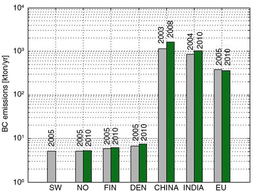
Fig. 2 Comparison of per capita BC emissions from DFNS, EU and the world's largest emitters – China and India.

3. Description of the model and observations

3.1. ECHAM–HAMMOZ global climate model

The global aerosol-climate model ECHAM-HAMMOZ (model version ECHAM6-HAM2.2-MOZ0.9) consists of the aerosol submodel HAM (Stier et al., 2005; Zhang et al., 2012) embedded in the global climate model ECHAM6 (Stevens et al., 2013). The atmospheric chemistry submodel MOZ is not used in the simulations described herein.

ECHAM6 consists of a spectral dynamic core that solves the vorticity and divergence form of the governing equations of motion of a hydrostatic atmosphere, together with a suite of physical parametrisations that represent diabatic and subgrid scale processes and a transport scheme for the advection of quantities other than temperature and surface pressure. For the simulations described herein, the model resolution is T63 (meaning triangular truncation of spherical harmonics at wave number 63), and the physical parametrisations are calculated on a Gaussian grid with 1.875 degrees resolution. In the vertical, the model domain extends from the surface to 10 hPa, with 31 levels. A hybrid sigma pressure vertical coordinate system is used, such that the near-surface levels are terrain-following, with gradual relaxation towards constant-pressure surfaces and decreasing vertical resolution with increasing distance from the surface. Tracer transport employs the flux-form semi-Lagrangian scheme of Lin and Rood (1996).

The aerosol submodel HAM represents the aerosol population as a set of seven lognormal size distributions modes, four of which consist of hydrophilic, internally-mixed particles and three of hydrophobic, externally-mixed particles. Historically, in publications that have employed the HAM model, the terms ‘soluble’ and ‘insoluble’ have been used instead of ‘hydrophilic’ and ‘hydrophobic’, and this terminology will be used hereafter. The size ranges are, in terms of dry particle diameter, 1–10 nm (nucleation mode) 10–100 nm (Aitken mode), 100 nm – 1 µm (accumulation mode) and >1 µm (coarse mode). Nucleation mode is not applicable to insoluble particles. Model species are sulphate (SO4), BC, OC, sea salt (SS) and mineral dust (DU). Prognostic variables for each mode are the geometric mean particle number concentration of each mode and the mass concentration of each species in each applicable mode. The geometric standard deviation of each mode is fixed, having values of 2.0 for the coarse modes and 1.59 for all others.

HAM simulates the full aerosol life cycle. It includes a simplified chemistry schemes for the formation of sulphuric acid from SO₂ and marine dimethyl sulphide (DMS) (Feichter et al., 1996), and for the oxidation of secondary organic aerosol (SOA) precursor gases into condensable species (O'Donnell et al., 2011). Aerosol microphysics (nucleation, condensation of sulphuric acid vapour, coagulation and water uptake) are calculated using the M7 (Vignati et al., 2004) module with extensions described in (Kazil et al., 2010). Removal of particles from the atmosphere by precipitation follows Croft et al. (2009), while in-cloud scavenging is according to Croft et al. (2010). Dry removal processes – dry deposition and sedimentation – are unchanged from the original HAM submodel described in Stier et al. (2005).

ECHAM-HAMMOZ calculates the snow albedo separately for land and sea ice. In both cases the snow is assumed to accumulate over the whole gridbox (i.e. there is no specific snow surface area). Moreover, the detailed snow physical properties, such as grain size, are not calculated (the approach is more bulk-alike). Over land, the calculations are based on the land-surface model JSBACH (Brovkin et al., 2013), which uses the snow-albedo approach by Dickinson et al. (1993). In this method, ageing of snow and solar zenith angle are taken into account. Ageing reduces the snow albedo and is influenced by different factors, such as the grain growth effect due to vapour diffusion, the effect near and at freezing of melt water, and the deposition of dust and soot. In other words, the model does not calculate explicitly the grain sizes, but uses a parameterisation for it. Moreover, in JSBACH, the last term, that is, the deposition effect, is estimated to be globally constant. For the sea ice covered with snow, ECHAM-HAMMOZ calculates a temperature dependent function, which can have albedo values between 0.5 and 0.8. This represents the control experiment (CONTROL) for which the relevant albedo equations are presented in the first column in Table 1. To include the effect of BC deposition from the HAM aerosol module on snow, two modified versions of ECHAM-HAMMOZ model were developed. One version includes only the pure snow without any deposition effects (CTRALB experiment). In this version, the JSBACH deposition effect was removed from the snow ageing factor (see the modified equation for F _a in Table 1). In the second version, the effect was also removed and replaced by the deposition of BC from HAM module (ALB experiment for which the albedo scheme modifications are listed in the second column in Table 1). This was achieved by calculating the accumulated BC concentration in snow using the total deposition flux of BC (wet and dry deposition+sedimentation). Two assumptions were made: firstly, the deposited BC is homogeneously distributed to the total snow pack of a gridbox, and secondly, the accumulation starts from zero when all the snow melts from a gridbox. To connect the HAM based BC concentration in snow to the model's albedo, the BC concentration in snow was further used as an input for a parameterisation based on measurements by Svensson et al. (2015). This parameterisation calculates the snow albedo when BC snow concentration (in ppm) is known. The parametrisation takes the form:1

Table 1. Description of the albedo schemes

Variable	Original equation	Modified equation
a ice
a T
a sn
a snaf
F a =
r 1=

The CONTROL experiment uses the albedo scheme listed in the first column. CTRALB uses the snow age factor F _a from the second column while the ALB experiment undergoes all the modifications entered in the second column.

a _ice is the snow albedo on ice, a _min =0.6 (minimum snow on ice albedo), a _max =0.8 (maximum snow in ice albedo), T _s is surface temperature, T _m =273.15 K (snow melting temperature), T _u =T _m −1 ° (upper limit for a _T calculations), a _bcr is the albedo reductions of BC from eq. (1), a _sn is the albedo over land, a _snm =0.95 (maximum albedo of fresh snow in the visible range), F _am =0.2 (maximal rel. reduction of snow albedo by ageing in the visible range), F _a is the snow age factor, a _sna =0.4 (maximal relative reduction of snow absorption by large solar zenith angle), a _snaf is the snow-albedo angle factor, a _snmin =0.15 [minimum albedo for (dirty) snow], z _z is the zenith angle, z _af =2 (factor in solar zenith angle dependence of snow albedo), r ₁ is the grain growth effect, is the additional effect near and at freezing of melt water, r _d is the effect of dirt and soot and sn _Δt is the snow fall per time step.

where a=−0.1566, b=0.5643 and c=0.858. However, the albedo from the above parameterisation cannot be directly used in the model, because the maximum value (i.e. pure snow albedo) is lower than in JSBACH. This would lead to overestimations of BC snow effect. To overcome this problem, we calculated the reduction of the albedo caused by BC in snow as the difference between the pure snow albedo [c in eq. (1)] and eq. (1) and subtract this reduction from the model's original albedo (snow on ice and land separately). This way, the BC albedo effect reduces the original albedo only if BC is deposited on snow.

3.2. Simulations

In order to explore the influence of BC emissions from DFNS, several model runs have been conducted. The simulation period was 12 yr starting from year 2000, with an initial spinup of 3 months.

1. CONTROL – A base case simulation with global BC emissions from AEROCOM,

2. BCDFNS0 – As the CONTROL simulation, but with anthropogenic emissions of BC in DFNS set to zero and AEROCOM emissions elsewhere,

3. BCA – As the CONTROL simulation with global anthropogenic BC emissions set to zero,

4. CTRALB – As the CONTROL simulation but taking into account only the pure snow without any deposition effect, and

5. ALB – As the CTRALB simulation where the albedo scheme takes into account the influence of BC in snow.

All the above model runs have been nudged towards ERA INTERIM analysis (Dee et al., 2011) in order to facilitate the detection of signatures of changes in specific process representations, however at the expense of losing their ability to simulate feedback influences on the large-scale model meteorology.

Emissions of anthropogenic BC, OC and SO₂ are according to the AEROCOM II suite (www.aerocom.met.no/emissions.html), with biomass burning monthly emissions according to GFEDv2 [van der Werf et al. (2006) and www.falw.vu/~gverf/GFED/GFED_v2/] and other anthropogenic emissions following Lamarque et al. (2010). Emissions of SS, DU, DMS and biogenic SOA precursors are calculated online (Zhang et al., 2012).

3.3. Measurement data description

Given the uncertainties in model estimates of BC atmospheric concentrations (Forster et al., 2007), it is highly advantageous to use in–situ measurement data to compare to the model predictions. Long-term observational datasets for BC in DFNS are quite limited, making it challenging to reliably evaluate the model. Nevertheless, EBAS, a database hosting observation data of atmospheric composition and physical properties (Tørseth et al., 2012), provides two long-term datasets located in DFNS, namely Hyytiälä, Finland (Virkkula et al., 2011), and Zeppelin Mountain, Norway (Eleftheriadis et al., 2009), for the period 01.01.2005–31.12.2010. These datasets together with a series of 1 yr-long records of BC measured concentrations datasets around Europe as part of EMEP EC-OC campaign held in 2002–2003 (Simpson et al., 2007; Yttri et al., 2007) allow us to investigate the model performance with respect to BC. The majority of the sites listed in Table 2 are rural background sites, with only Edinburgh (UK) and Gent (Belgium) being of urban background.

Table 2. Measurement sites used in this study

Station	Country	Latitude	Longitude	Altitude (m)	Notes
Aspvetren	Sweden	58.80	17.38	20	^a
Belogna	Italy	44.48	11.33	0	^a,c
Braganca	Portugal	41.82	6.77	691	^a
Edinburgh	United Kingdom	55.95	3.21	0	^a,c
Gent	Belgium	51.05	3.72	0	^a
Hyytiälä	Finland	61.85	24.28	181	^b
Illmitz	Austria	47.77	16.77	117	^a
Ispra	Italy	45.80	8.63	209	^a
Kollumerwaard	the Netherlands	53.33	6.28	1	^a
Kosetice	Czech Republic	49.58	15.08	534	^a
Langenbrügge	Germany	52.80	10.76	74	^a
Mace Head	Ireland	53.33	9.90	25	^a
Mt. Zeppelin	Norway	78.9	11.88	474	^b
Virolahti	Finland	60.53	27.69	8	^a

^aEMEP EC-OC campaign, 1 July 2002–1 July 2003, 24 h filter measurements of EC, weekly, details in Yttri et al. (2007).

^bData from ebas.nilu.no, aethalomether, 01.01.2005–31.12.2010.

^cPart of the EMEP EC-OC campaign, but not described in Yttri et al. (2007).

4. Results

4.1. Comparison to observations

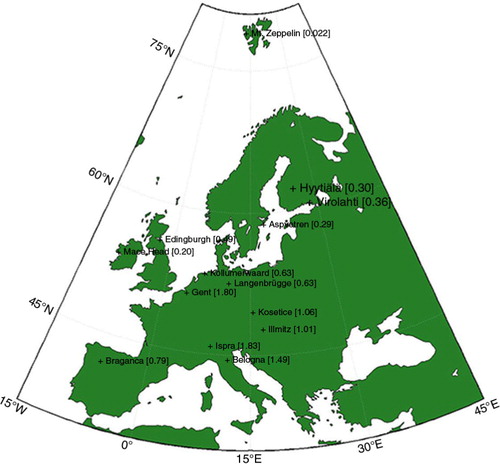
The spatial distribution of the measurement sites is presented in Fig. 3, together with the mean surface BC concentrations over the entire sampling period. A pronounced North to South BC concentration gradient is observed. The lowest concentrations were found in the Nordic countries and Ireland, increasing up to two orders of magnitude towards Southern, Eastern and Central European sites, showing that the rural backgrounds in continental Europe are more affected by the urban areas than those situated at the periphery of Europe. The level of BC concentration measured at Ispra (Italy) exceeds the concentrations recorded at any other rural and urban background site. This is most likely due to its location in the vicinity of the very polluted Po Valley.

Fig. 3 The location of the measurement sites. The numbers between the brackets represents the mean surface BC concentration for the entire measurement period.

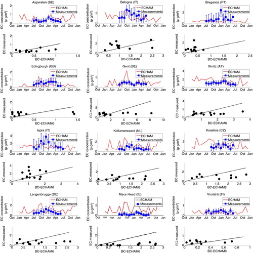
Figure 4 illustrates the time series and the scatter plots of the monthly mean BC concentrations for the 1-yr datasets around Europe. The model is reproducing the variability of the individual observations within 1–2 standard deviations of the measurements, especially in the region this study is focused on. There are some cases of underestimation by approximately a factor of 2 [Belogna (IT), Braganca (PT), Edinburgh (GB), Ispra (IT)] as well as overestimation by the same factor [Aspvreten (SE), Kollumeewaard (NL)]. The largest overestimation occurs in Mace Head (IE), where the model means overestimated on average the observations by 185 %.

Fig. 4 Time series and scatter plots of monthly means of measured (blue square) and modelled (red line) BC surface concentrations from July 2002 to July 2003. The error bars represent the 2x standard deviation. The 1:1 line is drawn for clarity.

Figure 5 presents the observed and modelled BC monthly mean surface concentrations for the two long-term datasets in Hyytiälä (FI) and Zeppelin Mountain (NO). On average, the model overestimates by 20 %the concentrations of BC in Hyytiälä (0.3±0.12 µg/m³ in the measurements and 0.36±0.26 µg/m³ in the model), while in Zeppelin Mountain the overall observed mean BC concentration (0.022±0.02 µg/m³) is underestimated by the model (0.015±0.02 µg/m³) by about 31 %. In addition, the model is about 3–4 months out of phase with the observations in the Zeppelin Mountain. This phase shift is not unprecedented. Many models failed to simulate a realistic seasonal cycle in this particular location. For instance, Shindell et al. (2008) compared 13 models with BC and sulphate mass concentrations at Svalbard, Alert and Barrow and found that in almost half of the models the sulphate concentration was 3–6 months out of phase with the measurements. Korhonen et al. (2008) compared aerosol size distribution measurements with model results at Zeppelin Mountain (in Svalbard) and encountered also a seasonal phase shift. Both studies found that the aerosol concentrations are very sensitive to the modelled deposition rates. Browse et al. (2012), using a global aerosol microphysics model (GLOMAP) and surface aerosol measurements, improved the agreement between model and observation and corrected the modelled seasonal cycle by introducing two new deposition parameterisations, ice-cloud and low cloud scavenging.

Fig. 5 Time series and scatter plots of monthly means of measured (blue square) and modelled (red line) BC surface concentrations from January 2005 to December 2010. The error bars represent the 2x standard deviation. The 1:1 line is drawn for clarity.

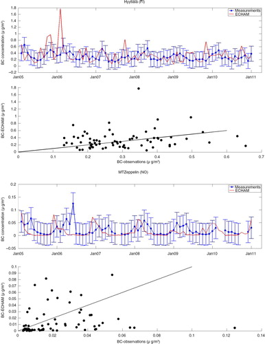
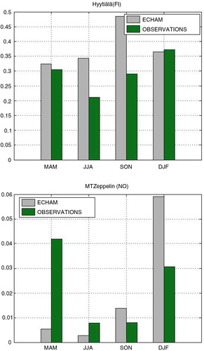
Both simulations and observations present a certain seasonal variability for BC surface concentrations, better observed in Zeppelin Mountain. However, the model results do not reproduce the measured seasonal cycle, as reflected in Fig. 6. The seasonality of the BC concentrations is determined by the seasonality of the emissions, meteorological conditions and removal processes. In this study the anthropogenic BC emissions are considered constant through the year while the biomass burning emissions have a maximum in the summer and a winter minimum. However, the model results present a maximum in autumn in Hyytiälä and winter in Zeppelin Mountain and minimum during spring and summer for both stations. This may be due to more efficient ventilation during the warm seasons due to stronger vertical mixing and stronger surface winds. At Hyytiälä the winter and spring model results and site measurements agree very well while for summer and autumn the model overestimates the observations by 35 and 38 %, respectively. At Zeppelin Mountain, data-model comparison highlights significant differences during the winter and spring months. During these periods, frequent episodes of high (in comparison to the yearly average) BC concentrations are observed (Fig. 5). Eleftheriadis et al. (2009) (and the references within) considered that measured BC seasonal cycle at Zeppelin Mountain is generally attributed to the seasonal position of the Arctic polar front. During the winter, the polar front lies at about 50 °N allowing long-range transport from major industrial regions in Europe, Russia and North America into the Arctic while during the summer the front is located at about 70 °N, preventing polluted air masses from reaching the Arctic. In comparison, the model results show a winter overestimation by a factor of 2 and a strong spring underestimation by a factor of 8. The modelled summer underestimation and the autumn overestimation are both by a factor of 2.

Fig. 6 Observed and modelled seasonal mean BC surface concentrations (µg/m³) in Hyytiälä in the upper panel and Zeppelin Mountain in the lower panel (DJF=Dec–Feb, MAM=Mar–May, JJA=Jun–Aug, SON=Sep–Nov).

In summary, ECHAM-HAMMOZ model is generally reasonable in reproducing the BC surface concentrations in the stations around Europe, but fails to simulate the observed seasonal cycle in some stations, especially at Zeppelin Mountain where insufficient BC mass in the spring and too much BC in the winter is simulated. The bias might be due to the incapacity of the model to resolve meteorological processes reflected by the measurements at local scale, as well as the inter-seasonal and inter-annual variabilities of the anthropogenic BC emissions. Nevertheless, the model results are sufficiently accurate in terms of BC concentrations averaged over long periods of time and can be used for further analysis.

4.2. Modelling results

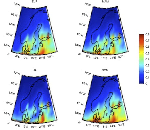
The continuous 12-yr CONTROL model simulation delivers the annual and seasonal cycle of the BC surface concentrations over DFNS. The seasonal average spatial distribution of BC surface concentrations (Fig. 7) is characterised by higher BC concentrations in Southern DFNS around locations with dense population and intensive industrial activities and lower BC concentrations towards North. The large North to South concentration gradient is common for all seasons and corresponds to the BC emission pattern. Same figures reveal that BC concentrations reach a maximum during the autumn (an average of 0.25 µg/m³) and a minimum during the summer (0.17 µg/m³), the seasonal gap being more evident around the areas with higher BC concentrations.

Fig. 7 Spatial distribution of BC surface concentrations seasonal mean (µg/m³) (DJF=Dec–Feb, MAM=Mar–May, JJA=Jun–Aug, SON=Sep–Nov).

Radiative forcing has become the standard metric to quantify the potential climate impact of various aerosols and greenhouse gases on a global or regional scale. In consonance with the metric, the averaged short-wave (SW) top of the atmosphere (TOA) clear-sky and total-sky radiative forcing over DFNS when removing the anthropogenic emissions from this area (calculated as the difference between 12 yr average CONTROL and BCDFNS0 experiments and denoted henceforth as ΔBCDFNS0) is presented in Fig. 8. BC introduces a positive forcing from a local minimum of 0.5 mW/m² to a maximum of 47 mW/m² for clear sky and from −34.1 mW/m² to 57.9 mW/m² for total sky. Due to the reduced amount of solar radiation during the cold seasons and the larger insolation during the long days of spring and summer, there is also a significant seasonal variability in the estimates of the BC TOA radiative forcing. The average values for the cold season are 5.7 mW/m² (clear sky) and 4 mW/m² (total sky) and 31 mW/m² (clear sky) and 36 mW/m² (total sky) for the warm seasons (Figs. 9 and 10). The SW clear-sky radiative forcing calculated at the surface is negative, having the largest contribution in the summer (−150 mW/m²) and smallest in the winter (−22 mW/m²), with a total mean value of −82.1±7 mW/m². The mean TOA SW clear-sky and total-sky radiative forcings of BC over DFNS obtained from ΔBCDFNS0 experiment (16.2±1.4 mW/m² and 18.7±2.4 mW/m², respectively) are about eight times smaller than the radiative forcing over the same area obtained from ΔBCA experiment (129.3±11.5 mW/m² and 202.4±12.8 mW/m²) in which all global anthropogenic emissions are switched off. Here ΔBCA represents the difference between BCA experiment and CONTROL.

Fig. 8 Twelve years mean TOA clear-sky (upper) and total-sky (lower) BC radiative forcing over DFNS (W/m²) from the ΔBCDFNS0 experiment where the BC anthropogenic emissions in DFNS area have been set to zero.

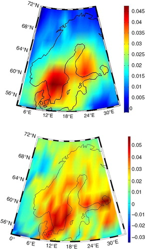
Fig. 9 Seasonal TOA SW clear-sky BC radiative forcing over DFNS (W/m² from the ΔBCDFNS0 experiment where the BC anthropogenic emissions in DFNS area have been set to zero). (DJF=Dec–Feb, MAM=Mar–May, JJA=Jun–Aug, SON=Sep–Nov).

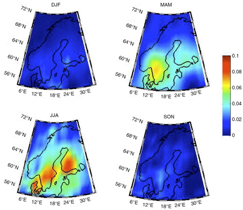
Fig. 10 Seasonal TOA SW total-sky BC radiative forcing over DFNS (W/m² from the ΔBCDFNS0 experiment where the BC anthropogenic emissions in DFNS area have been set to zero). (DJF=Dec–Feb, MAM=Mar–May, JJA=Jun–Aug, SON=Sep–Nov).

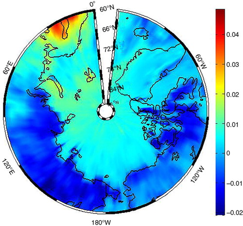
The mean TOA SW clear-sky radiative forcing caused by DFNS black carbon emissions over the Arctic (defined here from 60 to 90 °N) is illustrated in Fig. 11. The 12-yr-mean radiative forcing of 2.9±0.28 mW/m², with negligible values during the polar winter and reaching a maximum of 8 mW/m² when the insolation is substantial, represents 2 % of the TOA radiative forcing from the global anthropogenic emissions (ΔBCA) calculated over the same period of time (133.4±11.5 mW/m²). The total BC TOA forcing over the Arctic is consistent with the values obtained by Quinn et al. (2011) using NCAR-CAM4 and Oslo-CTMx models (120 and 140 mW/m², respectively), but smaller than the estimated Arctic BC+OC forcing of 400 mW/m² by Bond et al. (2011) and 550 mW/m² by Flanner et al. (2009). The mean TOA SW total-sky radiative forcing over Arctic from the ΔBCDFNS0 and ΔBCA experiments have higher values than their corresponding clear-sky values (8.6±1.41 mW/m² and, respectively, 162±19.3 mW/m²). It is known that a polar dome (defined as the surfaces of constant potential temperature that isolate the cold lower troposphere from the rest of the atmosphere) forms over the Arctic regions (Quinn et al., 2011) extending to about 40 °N (not symmetric). The dome can make the northern Eurasian emissions a major source for the Arctic BC (Stohl, 2006). The impact that our model shows for Arctic depends on how realistically the transport and sink processes are described. Earlier studies have shown (e.g. Croft et al., 2010) that the model has some deficiencies in BC sinks (removal being too efficient), which could lead to underestimations of DFNS Arctic BC forcing. This indicates that the DFNS emissions could have a bigger role for Arctic climate than shown here.

Fig. 11 TOA SW clear-sky BC radiative forcing over Arctic (W/m²) from the ΔBCDFNS0 experiment where the BC anthropogenic emissions in DFNS area have been set to zero.

The clear-sky and total-sky BC radiative forcing in ΔBCDFNS0 at global level were determined (0.04±0.022 mW/m² and 0.046±0.023 mW/m², respectively) as the product of the BC radiative forcing in ΔBCDFNS0 at DFNS zone and the ratio of the DFNS and global surface areas. Due to the ‘unorthodox’ way of calculating, it should be regarded as an indicator rather than an absolute value of the impact of BC anthropogenic emissions from DFNS on global climate. This impact can be examined also from the radiative forcing per capita (a measure similar to the carbon footprint) point of view. Considering an average population of 20 million in DFNS and 6.5 billion globally, we found that the DFNS per capita clear-sky radiative forcing in ΔBCDFNS0 experiment of about 0.8 nW/(m² cap) is one order of magnitude larger that the global per capita radiative forcing in BCA experiment of 0.023 nW/(m² cap).

The 12-yr mean values of total-sky radiative forcing caused by BC in both ΔBCDFNS0 and ΔBCA experiments are higher (yet still comparable) to those of the clear sky, but the range of the variation is about two times larger than those of clear-sky forcings. Moreover, the spatial distribution of the BC total-sky forcing is more scattered when compared to the clear-sky ones. These results hint towards an enhancement of the BC radiative forcing by clouds.

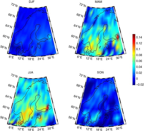
In addition to the atmospheric radiative effect discussed above, the presence of soot particles in snow causes a decrease in the albedo of snow and exerts a positive radiative forcing. There are two main factors affecting the mean radiative effects caused by BC in snow in a certain region: the concentration of BC in snow and the evolution of the snow cover, leading to large seasonal variations. The surface albedo forcing (accounting only for snow and ice covered areas) is calculated as the mean difference between radiative fluxes for clean snow (the CTRALB run) and for snow/ice containing BC (ALB experiment) denoted here by ΔALB. The BC in snow and ice forcing estimate in this paper (117±9.8 mW/m² globally averaged over 12 yr) is comparable to the current model estimates of global present-day BC-in-snow forcing that span from 3 to 110 mW/m² (Jacobson, 2004; Hansen et al., 2005; Flanner et al., 2007, 2009; Koch et al., 2009; Rypdal et al., 2009; Bond et al., 2011) (Fig. 12). The snow/ice forcing by BC is largest during the spring (290 mW/m²) while spatially, the midlatitude radiative forcings have larger values than those in Arctic and over DFNS (Fig. 13). Within DFNS, the averaged forcing due to BC in snow is greater than the global mean (145±27.2 mW/m²) while within the Arctic the radiative forcing reaches 81.4±9.7 mW/m². When calculating the BC-in-snow forcing with BC emissions in DFNS set to 0 [calculated from ALB-(ALB-DFNS emissions)], the signal obtained decays below the level of noise and no coherent values can be retrieved. Therefore, we estimated the influence level of BC emissions in DFNS on BC-in-snow forcing by multiplying the BC-in-snow forcing from ΔALB experiment with the ratio of the deposition fluxes calculated in BCDFNS0 and CONTROL and subtracting this product from the BC-in-snow forcing from ΔALB experiment. Although this is a simple calculation (denoted by ALBDFNS0), it provides at least a semi-quantitative estimation of the BC-in-snow forcings from the regional BC contributions to each receptor sites. As expected, the removal of BC emissions from DFNS area decreases the radiative forcing on snow values by 12 % (17.3±3.34 mW/m²) in DFNS, by 5 % (4.2±0.77 mW/m²) over the Arctic and by as much as 3.6 % (0.042±0.012 mW/m²) globally. The removal of BC anthropogenic emissions from DFNS generates responses of same order of magnitude in both radiative forcing due to BC in the atmosphere and due to BC-in-snow, as it can be seen in Table 3 where a summary of the results for each experiment and area of interest is presented. Reducing the BC emissions during cold seasons will affect mainly the snow radiative forcing. During the warm seasons, a decrement of BC would cause a reduction in the direct radiative forcing, leading to a cooling effect, effect that could be diminished or even counterbalanced by the reduction of the co-emitted OC, which is generally thought to have a direct cooling effect, by reflecting incoming sunlight.

Fig. 12 BC in snow and ice forcing (W/m²) averaged over 12 yr (2000–2011) from the ΔALB experiment.

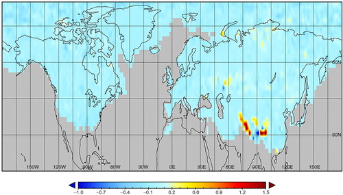
Fig. 13 Seasonal BC in snow and ice forcing (W/m²) averaged over 12 yr (2000–2011) from the ΔALB experiment (DJF = Dec–Feb, MAM = Mar–May, JJA = Jun–Aug, SON = Sep–Nov).

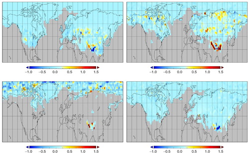
Table 3. Mean SW clear-sky (CS), total-sky (TS) and BC-in-snow (BCs) radiative forcing (mW/m²) from ΔBCDFNS0, ΔBCA, ΔALB and ALBDFNS0 experiments over DFNS, Arctic and at global level

CS/TS/BCs	Exp/Area	DFNS	Arctic	Global
CS	ΔBCDFNS0	16.2±1.4	2.9±0.28	0.04±0.022
	ΔBCA	129.3±11.5	133.4±15.5	151.5±4.2
TS	ΔBCDFNS0	18.7±2.4	8.6±1.41	0.046±0.023
	ΔBCA	202.4±12.8	162±19.3	191.5±8.2
BCs	ΔALB	145±27.2	81.4±9.7	117.5±9.8
	ALBDFNS0	17.3±3.34	4.2±0.77	0.042±0.012

5. Conclusions

This study provides an assessment of the climate impact of BC emitted in DFNS on DFNS itself, on the Arctic and globally. Our tool of choice was the climate global model ECHAM6-HAMMOZ ran for 12 yr starting with year 2000 and constrained by meteorological measurements. Studies of BC emission conducted at national level showed that, on average, the emission rates remained constant in the last 1.5 decades, with BC emissions from the domestic sector being the main BC contributor. The magnitude of the estimated emission rates in DFNS is 2–3 orders of magnitude smaller than the largest BC source countries (India and China) and only 6 % of the European emission capacity. The AEROCOM emission database used in this study falls within the same order of magnitude as the estimated rates.

The climate impact of DFNS BC was evaluated by switching off entirely the anthropogenic emissions on DFNS territory and 12 yr of simulation (BCDFNS0) were performed using the same meteorological fields as in the control run (with the BC emissions intact). The signal was calculated as the difference between the two runs. The overall TOA SW clear-sky BC radiative forcing over DFNS is 16.2±1.4 mW/m², with slightly higher values over the southern part of the domain. At global level, the BC emitted in DFNS contributes to the radiative forcing with as much as 0.04±0.022 mW/m². The DFNS radiative forcing per capita is one order of magnitude larger than the global average per capita. At the surface, the BC radiative forcing is negative.

Our calculations show that the BC-in-snow forcing appears to be as big as the direct BC radiative forcing. Because the BC emissions are mostly from household heating, thus mostly during the winter time, we conclude that the reduction of household wood burning could be the most effective mitigation strategy.

For regions like Scandinavia with a long history of mitigation policy that actually led to a considerable decrease in atmospheric BC load and which exhibit a relatively low emission intensity, there is still potential for further reduction, especially in the domestic sector. However, the degree of pollution is not dictated by the region's own emissions, but is also a transboundary problem. Our approach did not consider the influence of BC emissions from outside DFNS, but it is probably worth mentioning at this point. While both long-range transport and local and regional sources contribute to the surface BC concentrations, it is expected that less populated areas are dominated by long-range transported BC, as Hienola et al. (2013) pointed out. At the European level, the transboundary BC is expected to decrease due to the environmental legislation and activities of European Union. This is specifically true for the closest new EU-members – the Baltic countries. A possible issue for the long-range transport of BC in DFNS is Russia, which faces a much weaker political and legal pressure for emission decrease.

Capturing the impact of BC from DFNS (and generally from any region) is not necessarily only a scientific matter, but also a policy question. The present study values the climate damage associated with DFNS BC to be non-negligible, especially when compared to per capita global averages. As such, policy-makers may consider continuing their efforts in pursuing the BC reduction as part of a larger strategy for near-term as well as long-term climate change.

6. Acknowledgements

We thank the anonymous reviewers for their careful reviews and suggestions that helped to greatly improve the analyses and discussion presented in this paper. The ECHAM-HAMMOZ model is developed by a consortium composed of ETH Zurich, Max Planck Institut fr Meteorologie, Forschungszentrum Jlich, University of Oxford, and the Finnish Meteorological Institute and managed by the Center for Climate Systems Modeling (C2SM) at ETH Zurich. All the contributors to the black carbon measurements are warmly acknowledged. We would like to thank Academy of Finland (COOL, project 140867, and projects 250348 and 256208) and to PEGASOS project funded by the European Commission und the Framework Program 7 (FP7-ENV-2010-265148) for the financial support.

References

- Aasestad K . Emissions of Black Carbon and Organic Carbon in Norway 1990–2011. 2013. Technical Report, Statistics Norway. Online at: https://www.ssb.no/en/natur-og-miljo/artikler-og-publikasjoner/emissions-of-black-carbon-and-organic-carbon-in-norway-1990-2011 .
- Amann M. , Borken-Kleefeld J. , Cofala J. , Hettelingh J.-P. , Heyes C. , co-authors . The Final Policy Scenarios of the EU Clean Air Policy Package – TSAP Report 11. 2014; Belgium: Technical Report, IIASA.
- Bahadur R. , Feng Y. , Russel L. M. , Ramanathan V . Impact of California's air pollution laws on black carbon and their implications for direct radiative forcing. Atmos. Environ. 2011; 45(5): 1162–1167. http://dx.doi.org/10.1016/j.atmosenv.2010.10.054 .
- Bond T. , Doherty S. J. , Fahey D. W. , Forster P. , Berntsen T. , co-authors . Bounding the role of black carbon in the climate system: a scientific assessment. J. Geophys. Res. 2013; 16: 5380–5552. http://dx.doi.org/10.1002/jgrd.50171 .
- Bond T. , Zarzycki C. , Flanner M. , Koch D. M . Quantifying immediate radiative forcing by black carbon and organic matter with the specific forcing pulse. Atmos. Chem. Phys. 2011; 11: 1505–1525.
- Bond T. C. , Streets D. , Yarber K. , Woo J. , Klimont Z . A technology-based global inventory of black and organic carbon emissions from combustion. J. Geophys. Res. Atmos. 2004; 109: 14203. http://dx.doi.org/10.1029/2003JD003697 .
- Brovkin V. , Boysen L. , Raddatz T. , Gayler V. , Loew A. , co-authors . Evaluation of vegetation cover and land-surface albedo in MPI-ESM CMIP5 simulations. J. Adv. Model. Earth Syst. 2013; 5(1): 48–57. http://dx.doi.org/10.1029/2012MS000169 .
- Browse J. , Carslaw K. S. , Arnold S. R. , Pringle K. , Boucher O . The scavenging processes controlling the seasonal cycle in arctic sulphate and black carbon aerosol. Atmos. Chem. Phys. 2012; 12: 6775–6798.
- Croft B. , Lohmann U. , Martin R. , Stier P. , Wurzler S. , co-authors . Influences of in-cloud aerosol scavenging parameterizations on aerosol concentrations and wet deposition in ECHAM5-HAM. Atmos. Chem. Phys. 2010; 10: 1511–1543.
- Croft B. , Lohmann U. , Martin R. V. , Stier P. , Wurzler S. , co-authors . Aerosol size-dependent below-cloud scavenging by rain and snow in the ECHAM5-HAM. Atmos. Chem. Phys. 2009; 9: 4653–4675.
- Dee D. P. , Uppala S. M. , Simmons A. J. , Berrisford P. , Poli P. , co-authors . The ERA-interim reanalysis: configuration and performance of the data assimilation system. Q. J. Roy. Meteorol. Soc. 2011; 137: 553–597. http://dx.doi.org/10.1002/qj.828 .
- Dickinson R. , Henderson-Sellers A. , Kennedy P . Biosphere–Atmosphere Transfer Scheme (BATS) Version 1e as Coupled to the NCAR Community Climate Model. 1993. NCAR Tech. Note NCAR/TN-387+ STR. DOI: http://dx.doi.org/10.5065/D67W6959 .
- Eleftheriadis K. , Vratolis S. , Nyeki S . Aerosol black carbon in the European Arctic: measurements at Zeppelin station, Ny-ålesund, Svalbard from 1998 – 2007. Geophys. Res. Lett. 2009; 36(L02): 809. http://dx.doi.org/10.1029/2008GL035741 .
- USEPA . Report to Congress on Black Carbon. 2012. Technical Report. Department of the Interior, Environment, and Related Agencies Appropriations Act, 2010, United States Environmental Protection Agency (US EPA). Online at: http://epa.gov/blackcarbon/ .
- Feichter J. , Kjellström E. , Rodhe H. , Dentener F. , Lelieveld J. , co-authors . Simulation of the tropospheric sulfur cycle in a global climate model. Atmos. Environ. 1996; 30: 1693–1707.
- Flanner M . Arctic climate sensitivity to local black carbon. J. Geophys. Res. 2013; 118(4): 1840–1851. http://dx.doi.org/10.1002/jgrd.50176 .
- Flanner M. , Shell K. , Barlage M. , Perovich D. , Tschudi M . Radiative forcing and albedo feedback from the northern hemisphere cryosphere between 1979 and 2008. Nat. Geosci. 2009; 4: 151–155.
- Flanner M. , Zender C. , Randerson J. , Rasch P . Present-day climate forcing and response from black carbon in snow. J. Geophys. Res. 2007; 112: 11202. http://dx.doi.org/10.1029/2006JD008003 .
- Forsberg T. , Mikkola-Pusa J. , Petäjä J. , Saarinen K . Air Pollutant Emissions in Finland 1980–2012 Informative Inventory Report to the UNECE CLRTAP. 2014; Finland: Technical Report, Finnish Environment Institute.
- Forster P. , Hegerl G. , Knutti R. , Ramaswamy V. , Solomon S. , co-authors . Assessing uncertainty in climate simulations. Nature. 2007; 4: 63–64. http://dx.doi.org/10.1038/climate.2007.46a .
- Hansen J. , Nazarenko L . Soot climate forcing via snow and ice albedos. Proc. Natl. Acad. Sci. U S A. 2004; 101(2): 423–428.
- Hansen J. , Sato M. , Ruedy R. , Nazarenko L. , Lacis A. , co-authors . Efficacy of climate forcings. J. Geophy. Res. 2005; 110: 18104. http://dx.doi.org/10.1029/2005JD005776 .
- Hansson H.-C. , Johansson C. , Nyqvist G. , Kindbom K. , Åöm S. , co-authors . Black Carbon – Possibilities to Reduce Emissions and Potential Effects. 2011. Technical Report, Department of Applied Environmental Science. Online at: http://www.ivl.se/download/18.5c577972135ee95b56380001508/1350484317856/B2049.pdf .
- Hienola A. I. , Pietikäinen J.-P. , Jacob D. , Pozdun R. , Petäjä T. , co-authors . Black carbon concentration and deposition estimations in Finland by the regional aerosol–climate model REMO-HAM. Atmos. Chem. Phys. 2013; 13: 4033–4055. http://dx.doi.org/10.5194/acp-13-4033-2013 .
- Jacobson M. Z . Climate response of fossil fuel and biofuel soot, accounting for soot's feedback to snow and sea ice albedo and emissivity. J. Geophys. Res. 2004; 109: 21201. http://dx.doi.org/10.1029/2004JD004945 .
- Janssen N. A. H. , Gerlofs-Nijland M. E. , Lanki T. , Salonen R. O. , Cassee F. , co-authors . Health Effects of Black Carbon. 2011; World Health Organization, Copenhagen, Denmark: Technical Report.
- Jiao C. , Flanner M. , Balkanski Y. , Bauer S. E. , Bellouin N. , co-authors . An AeroCom assessment of black carbon in Arctic snow and sea ice. Atmos. Chem. Phys. 2014; 14: 2399–2417. http://dx.doi.org/10.5194/acp-14-2399-2014 .
- Junker C. , Liousse C . A global emission inventory of carbonaceous aerosol from historic records of fossil fuel and biofuel consumption for the period 1860–1997. Atmos. Chem. Phys. 2008; 8: 1195–1207. http://dx.doi.org/10.5194/acp-8-1195-2008 .
- Kazil J. , Stier P. , Zhang K. , Quaas J. , Kinne S. , co-authors . Aerosol nucleation and its role for clouds and Earth's radiative forcing in the aerosol-climate model ECHAM5-HAM. Atmos. Chem. Phys. 2010; 10: 10733–10752. DOI: http://dx.doi.org/10.5194/acp-10-10733-2010 .
- Koch D. , Del Genio A. D . Black carbon semi-direct effects on cloud cover: review and synthesis. Atmos. Chem. Phys. 2010; 10: 7685–7696. DOI: http://dx.doi.org/10.5194/acp-10-7685-2010 .
- Koch D. , Schulz M. , Kinne S. , McNaughton C. , Spackman J. R. , co-authors . Evaluation of black carbon estimations in global aerosol models. Atmos. Chem. Phys. 2009; 9(22): 9001–9026. DOI: http://dx.doi.org/10.5194/acp-9-9001-2009 .
- Kopacz M. , Mauzerall D. , Wang J. , Leibensperger E. M. , Henze D. , co-authors . Origin and radiative forcing of black carbon transported to the Himalayas and Tibetan Plateau. Atmos. Chem. Phys. 2011; 11: 2837–2852. DOI: http://dx.doi.org/10.5194/acp-11-2837-2011 .
- Korhonen H. , Carslaw K. S. , Spracklen D. V. , Ridley D. A. , Strom J . A global model study of processes controlling aerosol size distributions in the arctic spring and summer. J. Geophys. Res. 2008; 113: 08211. DOI: http://dx.doi.org/10.1029/2007JD009114 .
- Kupiainen K. , Klimont Z . Primary Emissions of Submicron and Carbonaceous Particles in Europe and the Potential for their Control. 2004; Interim Report IR-04-79, International Institute for Applied Systems Analysis (IASA), Schlossplatz 1 A-2361 Laxenburg, Austria.
- Kupiainen K. , Klimont Z . Primary emissions of fine carbonaceous particles in Europe. Atmos. Environ. 2007; 41(10): 2156–2170. DOI: http://dx.doi.org/10.1016/j.atmosenv.2006.10.06 .
- Lamarque J.-F. , Bond T. , Eyring V. , Granier C. , Heil A. , co-authors . Historical (1850–2000) gridded anthropogenic and biomass burning emissions of reactive gases and aerosols: methodology and application. Atmos. Chem. Phys. 2010; 10: 7017–7039. DOI: http://dx.doi.org/10.5194/acp-10-7017-2010 .
- Lee Y. H. , Lamarque J.-F. , Flanner M. G. , Jiao C. , Shindell D. T. , co-authors . Evaluation of preindustrial to present-day black carbon and its albedo forcing from atmospheric chemistry and climate model intercomparison project (ACCMIP). Atmos. Chem. Phys. 2013; 13(5): 2607–2634. DOI: http://dx.doi.org/10.5194/acp-13-2607-2013 .
- Lin S.-J. , Rood R . Multidimensional flux-form semi-Lagrangian transport schemes. Mon. Weather Rev. 1996; 124: 2046–2070.
- Lu Z. , Zhang Q. , Streets D . Sulfur dioxide and primary carbonaceous aerosol emission in China and India, 1996–2010. Atmos. Chem. Phys. 2011; 11: 9839–9864.
- Mahmood R. , Li S . Remote influence of south Asian black carbon aerosol on East Asian summer climate. Int. J. Climatol. 2014; 34(1): 36–48. DOI: http://dx.doi.org/10.1002/joc.3664 .
- O'Donnell D. , Tsigaridis K. , Feichter J . Estimating the direct and indirect effects of secondary organic aerosols using ECHAM5-HAM. Atmos. Chem. Phys. 2011; 11: 8635–8659.
- Ohara T. , Akimoto H. , Kurokawa J . An Asian emission inventory of anthropogenic emission sources for period 1980–2020. Atmos. Chem. Phys. 2007; 7: 4419–4444.
- Quinn P. , Stohl A. , Arneth A. , Berntsen T. , Burkhardt J. , co-authors . The Impact of Black Carbon on Arctic Climate. 2011; Oslo: Technical Report, Arctic Monitoring and Assessment Program (AMAP).
- Reddy M. , Boucher O . Climate impact of black carbon emitted from energy consumption in the world's regions. Geophys. Res. Lett. 2007; 34: 11802. DOI: http://dx.doi.org/10.1029/2006GL028904 .
- Rypdal K. , Rive N. , Berntsen Z. , Klimont T. K. , Mideksa T. , co-authors . Costs and global impacts of black carbon abatement strategies. Tellus B. 2009; 61: 625–641.
- Sand M. , Berntsen T. K. , Kay J. , Lamarque J. F. , Seland Ø. , co-authors . The Arctic response to remote and local forcing of black carbon. Atmos. Chem. Phys. 2013b; 13: 211–224. DOI: http://dx.doi.org/10.5194/acp-13-211-2013 .
- Sand M. , Berntsen T. K. , Seland Ø. , Kristjansson J. E . Arctic surface temperature change to emissions of black carbon within Arctic or midlatitudes J. Geophys. Res. 2013a; 118(14): 7788–7798. DOI: http://dx.doi.org/10.1002/jgrd.50613 .
- Shindell D. , Chin M. , Dentener F. , Doherty R. , Faluvegi G. , co-authors . A multi-model assessment of pollution transport to the Arctic. Atmos. Chem. Phys. 2008; 8: 5353–5372.
- Simpson D. , Yttri K. , Klimont Z. , Kupiainen K. , Caseiro A. , co-authors . Modeling carbonaceous aerosol over Europe: analysis of the CARBOSOL and EMEP EC/OC campaigns. J. Geophys. Res. 2007; 112: 23S14. DOI: http://dx.doi.org/10.1029/2006JD008158 .
- Stevens B. , Giogetta M. , Esch M. , Mauritsen T. , Crueger T. , co-authors . Atmospheric component of the MPI-M Earth System Model: Echam6. J. Adv. Model. Earth Syst. 2013; 3(5): 146–172.
- Stier P. , Feichter J. , Kinne S. , Kloster S. , Vignati E. , co-authors . The aerosol-climate model ECHAM5-HAM. Atmos. Chem. Phys. 2005; 5: 1125–1156.
- Stohl A . Characteristics of atmospheric transport into the Arctic troposphere. J. Geophys. Res. Atmos. 2006; 11(D11): 2156–2202. DOI: http://dx.doi.org/10.1029/2005JD006888 .
- Streets D. , Gupta S. , Waldhoff S. , Wang M. , Bond T. , co-authors . Black carbon emissions in China. Atmos. Environ. 2001; 35: 4281–4296.
- Svensson J. , Virkkula A. , Meinander O. , Kivekäs N. , Hannula H.-R. , co-authors . Soot on snow experiments part 1: light-absorbing impurities effect on the natural snowpack. 2015. [Submitted to BER]..
- Textor C. , Schulz M. , Guibert S. , Kinne S. , Balkanski Y. , co-authors . Analysis and quantification of the diversities of aerosol life cycles within AeroCom. Atmos. Chem. Phys. 2006; 6(7): 1777–1813. DOI: http://dx.doi.org/10.5194/acp-6-1777-2006 .
- Tørseth K. , Aas W. , Breivik K. , Fjæraa A. M. , Fiebig M. , co-authors . Introduction to the European Monitoring and Evaluation Programme (EMEP) and observed atmospheric composition change during 1972–2009. Atmos. Chem. Phys. 2012; 12: 5447–5481. DOI: http://dx.doi.org/10.5194/acp-12-5447-2012 .
- van der Werf G. , Randerson J. , Giglio L. , Collatz G. J. , Kasibhatla P. S. , co-authors . Interannual variablility in global biomass burning emissions from 1997 to 2004. Atmos. Chem. Phys. 2006; 6: 3423–3441.
- Vignati E. , Wilson J. , Stier P . M7: an efficient size-resolved aerosol microphysics module for large-scale aerosol transport models. J. Geophys. Res. 2004; 109: 22202. DOI: http://dx.doi.org/10.1029/2003JD004485 .
- Virkkula A. , Backman J. , Aalto P. , Hulkkonen M. , Riuttanen L. , co-authors . Seasonal cycle, size dependencies, and source analyses of aerosol optical properties at the SMEAR II measurement station in Hyytiälä, Finland. Atmos. Chem. Phys. 2011; 11: 4445–4468. DOI: http://dx.doi.org/10.5194/acp-11-4445-2011 .
- Wang Q. , Jacob D. J. , Fisher J. A. , Mao J. , Leibensperger E. M. , co-authors . Sources of carbonaceous aerosols and deposited black carbon in the arctic in winter-spring: implications for radiative forcing. Atmos. Chem. Phys. 2011; 11(23): 112453–112473. DOI: http://dx.doi.org/10.5194/acp-11-12453-2011 .
- Wang R. , Tao S. , Balkanski Y. , Ciais P. , Boucher O. , co-authors . Exposure to ambient black carbon derived from a unique inventory and high-resolution model. PNAS. 2014; 111(7): 2459–2463. DOI: http://dx.doi.org/10.1073/pnas.1318763111 .
- Winther M. , Nielsen O.-K . Technology dependent BC and OC emissions for Denmark, Greenland and the Faroe Islands calculated for the time period 1990–2030. Atmos. Environ. 2011; 45: 5880–5895.
- Yttri K. E. , Aas W. , Bjerke A. , Cape J. N. , Cavalli F. , co-authors . Elemental and organic carbon in PM10: a one year measurement campaign within the European monitoring and evaluation programme EMEP. Atmos. Chem. Phys. 2007; 7: 5711–5725. DOI: http://dx.doi.org/10.5194/acp-7-5711-2007 .
- Zhang K. , O'Donnell D. , Kazil J. , Stier P. , Kinne S. , co-authors . The global aerosol-climate model ECHAM-HAM, version 2: sensitivity to improvements in process representations. Atmos. Chem. Phys. 2012; 12: 8911–8949.
- Zhang N. , Qin Y. , Xie S . Spatial distribution of black carbon in China. Chin. Sci. Bull. 2013; 58(31): 3830–3839. DOI: http://dx.doi.org/10.1007/s11434-013-5820-4 .