Decadal trends in the seasonal-cycle amplitude of terrestrial CO₂ exchange resulting from the ensemble of terrestrial biosphere models

Abstract

The seasonal-cycle amplitude (SCA) of the atmosphere–ecosystem carbon dioxide (CO₂) exchange rate is a useful metric of the responsiveness of the terrestrial biosphere to environmental variations. It is unclear, however, what underlying mechanisms are responsible for the observed increasing trend of SCA in atmospheric CO₂ concentration. Using output data from the Multi-scale Terrestrial Model Intercomparison Project (MsTMIP), we investigated how well the SCA of atmosphere–ecosystem CO₂ exchange was simulated with 15 contemporary terrestrial ecosystem models during the period 1901–2010. Also, we made attempt to evaluate the contributions of potential mechanisms such as atmospheric CO₂, climate, land-use, and nitrogen deposition, through factorial experiments using different combinations of forcing data. Under contemporary conditions, the simulated global-scale SCA of the cumulative net ecosystem carbon flux of most models was comparable in magnitude with the SCA of atmospheric CO₂ concentrations. Results from factorial simulation experiments showed that elevated atmospheric CO₂ exerted a strong influence on the seasonality amplification. When the model considered not only climate change but also land-use and atmospheric CO₂ changes, the majority of the models showed amplification trends of the SCAs of photosynthesis, respiration, and net ecosystem production (+0.19 % to +0.50 % yr⁻¹). In the case of land-use change, it was difficult to separate the contribution of agricultural management to SCA because of inadequacies in both the data and models. The simulated amplification of SCA was approximately consistent with the observational evidence of the SCA in atmospheric CO₂ concentrations. Large inter-model differences remained, however, in the simulated global tendencies and spatial patterns of CO₂ exchanges. Further studies are required to identify a consistent explanation for the simulated and observed amplification trends, including their underlying mechanisms. Nevertheless, this study implied that monitoring of ecosystem seasonality would provide useful insights concerning ecosystem dynamics.

• atmospheric carbon dioxide
• carbon cycle
• climate change
• land-use change
• seasonal cycle
• terrestrial ecosystem

To access the supplementary material to this article, please see Supplementary files under ‘Article Tools’.

1. Introduction

The carbon budget of terrestrial ecosystems is one of the most important mechanisms, in addition to anthropogenic emissions and ocean fluxes, that regulate atmospheric CO₂ concentrations (Le Quéré et al., 2015; Schimel et al., 2015). In particular, seasonal and interannual variabilities of atmospheric CO₂ concentrations (and sometimes their isotopic composition) are believed to be largely attributable to terrestrial sinks and sources. Inversely, terrestrial exchanges have been deduced from atmospheric observations such as temporal changes in the growth rate and seasonal-cycle amplitude (SCA: maximum range of oscillation within a calendar year between peak and trough) of atmospheric CO₂ concentration. The SCA of atmospheric CO₂ has been investigated in terms of interannual and longer changes in terrestrial ecosystem functions (e.g. Kohlmaier et al., 1989; Randerson et al., 1997; Schneising et al., 2014). On the basis of long-term observations, Graven et al. (2013) have recently indicated that the SCA of the northern atmospheric CO₂ concentration increased by 25–50 % over the last 50 yr. This finding is consistent with previous results reported by researchers such as Bacastow et al. (1985) and Keeling et al. (1996) but is associated with a higher level of confidence because it is based on novel analyses using long-term ground and aircraft data and atmospheric transport models. Recently, Forkel et al. (2016) implied that the increased SCA of atmospheric CO₂ and its latitudinal gradient is mainly caused by activation of photosynthetic uptake in northern vegetation, on the basis of terrestrial and atmospheric transport model simulations.

It has been hypothesized that climatic warming may stimulate the growth of middle- to high-latitude vegetation by ameliorating the effects of chilliness and elongating the growing season, although some harmful impacts (e.g. drought, insect outbreaks, wildfires, and increased decomposition) might partly offset the positive effects. Continuous monitoring of northern vegetation by remote sensing (e.g. Myneni et al., 1997; Barichivich et al., 2013) indicates that the photosynthetic activity of vegetation in these areas has been enhanced, the implication being that there has been greater CO₂ uptake during the growing period. Zhang et al. (2008) attempted to detect trends in northern vegetation productivity using satellite leaf area index (LAI) data and the fraction of absorbed photosynthetically active radiation from 1983 to 2005. In contrast, Xu et al. (2013) revealed that the SCA of the satellite vegetation index of northern ecosystems might have decreased, because more rapid warming trend in the winter may have lessened the seasonal contrast of temperature. Analysing space-borne atmospheric CO₂ data, Schneising et al. (2014) found a trend of declining SCA and obtained a negative correlation between the SCA and temperature anomaly, the implication being that that carbon uptake by vegetation was less efficient in a warmer climate. How the SCA of vegetation and ecosystem activities are changing and the underlying mechanisms accounting for the variation are therefore unclear.

Long-term monitoring of ecosystem structure and functions by means of ground-based remote sensing and micrometeorological flux measurement techniques would enable us to detect and analyse changes that would help to resolve these uncertainties. For example, continuous monitoring of leaf phenology (e.g. timings of leaf display and shedding; Richardson et al., 2013) provides useful data for quantifying these changes. Increasing amounts of continuous data on atmosphere–ecosystem CO₂ exchange are available from the worldwide network of tower-based observations made by the eddy-covariance method (global FLUXNET: Baldocchi et al., 2001). Several recent studies have attempted to scale up such observed flux data to a global-scale using sophisticated statistical methods (e.g. Jung et al., 2011). Nevertheless, there remain problems and uncertainties in temporal coverage, gap filling, bias correction, and quality control and assurance of observational data. Therefore, it is still difficult to assess broad-scale ecosystem functions and analyse their dynamics and underlying mechanisms using field observational data exclusively.

In this study, we analysed global-scale, long-term trends of the SCA of atmosphere–ecosystem CO₂ fluxes using data simulated by 15 contemporary terrestrial ecosystem models. First, we examined whether the models retrieved the SCA of fluxes and their historical trends to be consistent with observations. Second, we evaluated contribution of the potential mechanisms such as atmospheric CO₂, climate, land-use, and nitrogen deposition through factorial experiments. Remarkably, we could accomplish these analyses with higher credibility by using multiple-model experiments. A number of model intercomparison projects (MIPs) have been conducted to evaluate the range of the estimates for various metrics (e.g. Cramer et al., 1999; Sitch et al., 2008). It has been shown that each model has its own bias and that an ensemble of models is likely to provide less biased estimates of ecosystem dynamics. Based on multi-model simulation outputs, we examined whether a majority of the models with different environmental responsiveness simulated the SCA.

One of the advantages of such a simulation-based approach is that we can analyse a long-term trend such as an interannual-to-decadal change. Although the data that drive climate change and land use contain uncertainties, such simulation analyses have been conducted, for example, for the whole twentieth century (e.g. Post et al., 1997; Zeng et al., 2005; Piao et al., 2009) to reveal long-term dynamics. Also, by conducting a systematic sensitivity analysis, we may attribute the simulated changes to specific environmental driving factors. This capability is especially useful for separating the contributions of natural and anthropogenic components. An MIP-based analysis is apparently effective in evaluating the range of estimation uncertainty associated with different models. Several previous MIPs revealed that current global models, even though they were up-to-date, provided widely different results (Luo et al., 2015), the implication being that they are poorly constrained by observational data. In this study, we analysed time-series of the SCAs based on simulated gross (i.e. photosynthesis and respiration) and net CO₂ fluxes at global and regional scales. In terms of correspondence to the trend in atmospheric CO₂, apparently, net exchange and its seasonally accumulated fluxes are of great importance. Finally, we discuss the correspondence between the trends of terrestrial ecosystems and atmospheric CO₂, the potential limitations of this study, the implications for observation and future directions.

2. Data and methods

2.1. Data

We used data from the Multi-scale Synthesis and Terrestrial Model Intercomparison Project (MsTMIP), which was conducted as a part of the North American Carbon Program. The simulation protocol and preparation of the forcing data for the MsTMIP have been described in Huntzinger et al. (2013) and Wei et al. (2014). Using the same forcing data, we explored four global simulations: SG1, driven by climate data for the historical (1901–2010) period; SG2, similar to SG1, but including land-use change; SG3, similar to SG2, but including the rise of atmospheric CO₂; and BG1, similar to SG3, but including atmospheric nitrogen deposition. Each model was initialised through recursive calculation under the average climate condition in 1901–1930, so that the 100-yr mean ecosystem carbon-stock change comes sufficiently close to zero. Time-series data of atmospheric CO₂ concentration derived from observations (Wei et al., 2014) were applied to SG3; in other simulations, it was kept constant at the level of initialisation period. Therefore, by examining the differences between the factorial experiments, we could approximately assess the impact of specific forcing factors, foe example, the atmospheric CO₂ fertilization effect based on the difference between SG3 and SG2. In this study, climatic impacts were not separated into specific meteorological factors such as radiation, temperature, and precipitation. It is noteworthy that only a few models take into account nitrogen cycling in terrestrial ecosystems, and therefore, BG1 was conducted with a limited number of models. We expected that BG1 are SG3 were closest to the reality, and factorial separation was done for each model using available experimental results.

In this study, we used data from 15 terrestrial ecosystem models (Table 1) that submitted simulation data to the MsTMIP version 1 data set (www.nacp.ornl.gov/mstmipdata/). All the data had a spatial resolution of 0.5 °×0.5 ° in latitude and longitude. We intended to maximise the number of models to elucidate the range of inter-model variability. Monthly CO₂ flux data for SG1, SG2, SG3 and BG1 during the period 1901–2010 were therefore used in this study. When available, we used LAI data (LAI, m² m⁻²) for supplementary analyses to separate the contributions of physiological and structural responses in vegetation to the simulated amplification of the SCA of GPP.

Table 1. MsTMIP models and simulations used in this study

	Simulations
Model	SG1	SG2	SG3	BG1	References
BIOME-BGC	O			O	Thornton et al. (2002)
CLASS-CTEM-N^a	O	O	O	O	Huang et al. (2011)
CLM4	O	O	O	O	Shi et al. (2011), Mao et al. (2012)
CLM4VIC	O	O	O	O	Lei et al. (2014)
DLEM	O	O	O	O	Tian et al. (2011, 2012)
GTEC	O	O	O		Ricciuto et al. (2011)
ISAM	O	O	O	O	Jain and Yang (2005)
LPJ-wsl	O	O	O		Sitch et al. (2003)
ORCHIDEE-LSCE	O	O	O		Krinner et al. (2005)
SiB3-JPL	O	O	O		Baker et al. (2008)
SiB3CASA	O	O	O		Schaefer et al. (2008)
TEM6	O	O	O	O	Hayes et al. (2011)
TRIPLEX-GHG		O	O	O	Zhu et al. (2014)
VEGAS2.1	O	O	O		Zeng et al. (2005)
VISIT	O	O	O		Ito and Inatomi (2012)

See text for a description of simulations.

^aCalculated net CO₂ exchange was always negative and therefore not used.

Biome-BGC, Global Biome Model-Biogeochemical Cycle; MsTMIP Multi-scale Terrestrial Model Intercomparison Project (MsTMIP); CLASS-CTEM-N, Canadian Land Surface Scheme and Canadian Terrestrial Ecosystem Model with Nitrogen; CLM4, Community Land Model version 4; CLM4VIC, Community Land Model version 4 with Variable Infiltration Capacity Runoff Paramaterization; DLEM, Dynamic Land Ecosystem Model; GTEC, Global Terrestrial Ecosystem Carbon model; ISAM, Integrated Science Assessment Model; LPJ-wsl, Lund-Potsdam-June model by Swiss Federal Institute for Forest, Snow, and Landscape Research; ORCHIDEE-LSCE, Organising Carbon and Hydrology in Dynamic Ecosystems; SiB3-JPL: Simple Biosphere version 3 by Jet Propulsion Laboratory; SiBCASA, Simple Biosphere with Carnegie-Ames-Stanford Approach; TEM6, Terrestrial Ecosystem Model version 6; TRIPLEX-GHG, a process-based GHG model developed from three models; VEGAS2.1, Vegetation Global Atmosphere and Soil version 2.1; VISIT, Vegetation Integrative SImulator for Trace gases.

For a supplementary comparison, we used the global time-series data of Normalized Difference Vegetation Index (NDVI) produced by the Global Inventory Modeling and Mapping Studies (GIMMS) (NDVI3g: Zhu et al., 2013). Using the data from 1982 to 2010, we calculated the trend of SCA for each grid cell and compared with those of GPP simulated by the MsTMIP models. This comparison intended to examine the consistency of stimulated vegetation growth in the last 30 yr.

2.2. Analyses

This study focused on the SCA of atmosphere–ecosystem CO₂ exchange in relation to atmospheric CO₂ concentration.From the perspective of the global carbon budget, we conducted analyses first for global total fluxes and then for regional patterns. Although ecosystem responses and contributions may differ among regions, the global analyses are expected to clarify the dominant pattern and process most closely linked to the average trends in atmospheric CO₂. Because we used monthly data, changes in the seasonal phase (e.g. timing of transition from net release to uptake) and growing-season length (e.g. Barichivich et al., 2013) were not the central issue; these features should be considered in a forthcoming study. Note that simulations were conducted using 6-hourly meteorological data (Wei et al., 2014), and such sub-monthly vegetation responses were then implicitly included into CO₂ fluxes by most of the models. We ensured carefully that the net CO₂ budgets in terms of net ecosystem exchange (NEE) and net ecosystem production (NEP) were defined differently among the participating models (Zscheischler et al., 2014) with respect to land-use, fire, and product decay emissions. These ancillary carbon flows were small, but they can play key roles in the net carbon budget, trend analysis and seasonal CO₂ exchange (e.g. Zimov et al., 1999). Therefore, for clarity in this study, we adopted a unified definition of NEP as follows:1

where GPP is the gross primary production (photosynthetic uptake) and RE is the ecosystem respiration, which is the sum of autotrophic respiration from vegetation and heterotrophic respiration from soil decomposers. The NEP data calculated using eq. (1) (not those provided by each model group) were used in this study.

As shown by the idealized sample data in Fig. 1, seasonal changes in the difference between GPP and RE cause the seasonality of net atmosphere–ecosystem CO₂ exchange. Theoretically, a larger SCA in GPP and/or smaller amplitude of RE can lead to a larger SCA of net CO₂ exchange; a change in their seasonal-phase lag is also influential. Moreover, both the instantaneous flux rate and duration of flux are important in determining the impact of CO₂ fluxes on atmospheric CO₂ seasonality. The SCA was therefore evaluated using two metrics (see Fig. 1): (1) the SCA of the monthly flux (Fig. 1b), defined as the difference between the maximum and minimum monthly fluxes, and (2) the SCA of the cumulative flux (Fig. 1c), defined as the difference between the peak and trough of the cumulative flux for each calendar year. Many previous studies (e.g. Peng et al., 2015) adopted the former metric of SCA for net terrestrial CO₂ exchange. The latter metric for NEP, however, is expected to be more sensitive to ecosystem change, because it shows the difference accumulated over the growing period and throughout the year. Furthermore, the cumulative-flux metric is likely to be more directly related to changes in atmospheric CO₂ concentrations. Because gross fluxes (GPP and RE) always take positive values for each flux direction, their SCA was calculated using only the former definition. Note that additional metrics, such as the difference between growing- and dormancy-season total net fluxes (e.g. Gurney and Eckels, 2011), have been used for other research purposes. Figure 2 shows the average seasonality of monthly and cumulative global terrestrial NEP based on 15 models compared with the seasonality of global-mean atmospheric CO₂. Considering the fact that ocean and anthropogenic fluxes may have weak and different seasonality of atmospheric exchange, most of the terrestrial models are likely to simulate smaller SCAs of net CO₂ flux (e.g. Graven et al., 2013 for CMIP5 models; Peng et al., 2015 for TRENDY models). In contrast, seasonal phases in both monthly and cumulative fluxes are well correlated in most models (see Supplementary Fig. 1 for the global-mean atmospheric CO₂ data and their SCA trend).

Fig. 1 Explanation of seasonal-cycle amplitude (SCA) metrics with idealized sample data. (a) Seasonal change in gross CO₂ fluxes: GPP, gross primary production, and RE, ecosystem respiration. (b) Seasonal change in net CO₂ flux (NEP, net ecosystem production) and its seasonal amplitude. (c) Seasonal change in cumulative CO₂ flux in calendar year and its SCA.

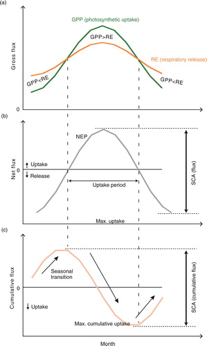
Fig. 2 Average seasonality of net ecosystem production estimated by 15 MsTMIP models and atmospheric CO₂ concentration. Global-mean atmospheric CO₂ data from 1984 to 2010 were obtained from the World Data Center for Greenhouse Gases (URL: http://ds.data.jma.go.jp/gmd/wdcgg/wdcgg.html). Model results of SG3 or BG1 (if available) for the same period were used. (a) Monthly net ecosystem production (positive for net sink) compared to monthly atmospheric CO₂ concentration change [i.e. Δ(CO₂)/Δt]. For both terrestrial fluxes and atmospheric CO₂, anomalies from the annual mean values are shown. (b) Cumulative net ecosystem production compared with seasonal changes in atmospheric CO₂ concentrations.

These metrics of the SCA were calculated for GPP, RE and NEP for different spatial extents: grid cell, latitudinal zone and global, respectively. The statistical significance of the linear trends was examined using the Student's t-test. In this study, three latitudinal zones were considered: tropical (25°S–25°N), northern middle (25°–55°N) and northern high (55°–90°N). From the time-series of SCA metrics calculated for each calendar year, linear trends were obtained by linear regression during specified periods. We focused especially on the contrast between the time intervals 1911–1960 and 1961–2010. The first 10 yr (1901–1910) of the study were not included to remove the transitional effects associated with the spin-up to the experimental phase.

3. Results

3.1. Global mean trends

In the MsTMIP simulations, terrestrial gross CO₂ fluxes increased at different rates among the models and simulations. In the SG1 simulations, global annual GPP increased from 113.3±26.3 Pg C yr⁻¹ [mean ±standard deviation (SD) for inter-model variability] in the 1910s to 113.8±27.1 Pg C yr⁻¹ in the 1960s and then to 116.3±27.4 Pg C yr⁻¹ in the 2000s. The GPP increase was more evident in the SG3 simulations: from 114.8±26.0 Pg C yr⁻¹ in the 1910s to 118.7±27.2 Pg C yr⁻¹ in the 1960s and then to 132.0±29.6 Pg C yr⁻¹ in the 2000s. The incremental trends in the SG2 simulations were comparable to those in the SG1 simulations, and those in BG1 were comparable with those in SG3. The global annual RE showed similar changes but the slope of trends was low, meaning slightly a weak trend.

In terms of model-ensemble results, the SCAs of global GPP and RE clearly increased over time, in parallel with the increase of annual (i.e. cumulative) fluxes (Fig. 3) in the SG3 and BG1 simulations. Although the amplification of GPP and RE offset each other (cf., Fig. 1a), the larger change of GPP seasonality resulted in seasonal amplifications of the estimated NEP. On average, the SCAs of cumulative NEP were estimated to be 5.8, 6.5, 7.3 and 6.5 Pg C (model average) in the 1950s for the SG1, SG2, SG3 and BG1 simulations, respectively. In the 2000s, the corresponding SCAs increased to 5.7, 6.8, 9.3 and 8.0 Pg C, respectively. The amplification of SCA was more evident in the SG3 and BG1 simulations than in the other simulations (Fig. 3). The difference between the SG2 and SG3 results was primarily attributable to the difference in atmospheric CO₂ concentrations, whereas the impact of land-use change accounted for only a small difference between the SG1 and SG2 results. The amplification of the SCA was almost proportional to the augmentation of the terrestrial CO₂ fluxes. Namely, the ratio of the SCA to the annual total flux was approximately constant through the simulation period. For GPP in the SG3 simulations, the magnitude of SCA was about 5.9 % of the annual flux in the 1910s and about 6.0 % in 2000s. Figure 4 also clarifies the fact that seasonality of the CO₂ flux was more amplified in SG3 through time. This pattern was especially apparent in the cumulative NEP, a pattern apparent in the average behaviour of all the MsTMIP models. Because the difference accumulated for several months during the growing period, the cumulative NEP showed clearer differences between the periods and simulations. Compared with SG1 and SG2 (Fig. 4b and d), the simulated NEP in SG3 (Fig. 4f) showed a clearer maximum uptake in NEP and peak cumulative uptake in September. A comparison between SG1 and SG2 (Fig. 4b and d) demonstrated that land-use change exerted a considerable influence on the seasonal change in atmosphere–ecosystem CO₂ exchange at the global scale.

Fig. 3 Interannual variability of the SCA of global terrestrial CO₂ fluxes. For each of the simulations (SG1, SG2, SG3 and BG1), model-average anomalies of the MsTMIP models against the 1950s-mean (grey zone) are shown. (a) Monthly GPP, (b) cumulative (i.e. annual total) GPP, (c) monthly RE, (d) cumulative RE, (e) monthly NEP and (f) cumulative NEP.

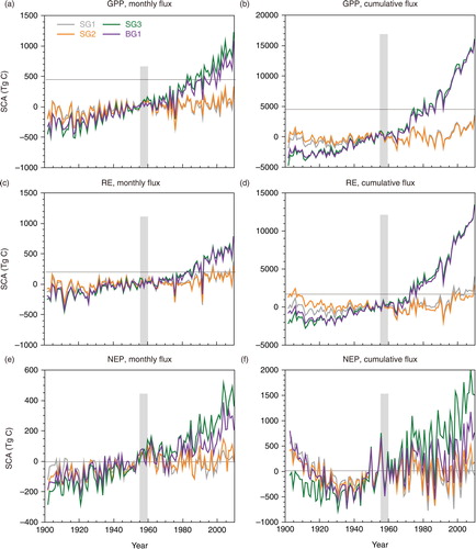
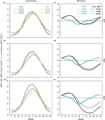
Fig. 4 Mean seasonal-cycle of gross and net CO₂ fluxes in the northern middle latitudinal zone (25–55°N) for different periods: the 1910s, 1950s and 2000s. Averages of MsTMIP model results for (a, b) SG1, (c, d) SG2 and (e, f) SG3 simulations.

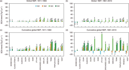
During the period 1961–2010 in the SG1, SG2, SG3 and BG1 simulations, model-ensemble linear trends of the SCA of cumulative global NEP were found to be −2.1±11.1, 5.0±12.2, 41.5±22.9 and 32.3±19.9 Tg C yr⁻¹, respectively. The relative incremental rates were found to be −0.02 %, +0.06 %, +0.50 % and +0.38 % yr⁻¹, respectively (Table 2). These trends of cumulative NEP were slightly larger than those of gross and net monthly fluxes: +0.19 % to +0.28 % yr⁻¹ (Table 2). Assuming the SG3 or BG1 results as a reference, it is possible to separate contributions of different factors by differentiating simulations. For example, climate, land-use change and atmospheric CO₂ rise contributed to the model-average SCA trend of cumulative NEP to −4.9 %, +17.8 % and +87.1 %, respectively, for the SG3 simulations. For the SCA trend of RE, climate change made a considerable contribution (+30.4 %).

Table 2. Simulated linear trends in the seasonal-cycle amplitude (SCA) of global terrestrial CO₂ fluxes

	Linear trend in SCA, 1961–2010 (% yr^−1)
Experiment	GPP	RE	NEP	Cum. NEP
SG1	+0.023	+0.068	−0.011	−0.024
SG2	+0.042	+0.062	+0.014	+0.064
SG3	+0.257	+0.222	+0.276	+0.496
BG1	+0.209	+0.209	+0.190	+0.382
Atmospheric CO2 trends
Global mean (1984–2010)^a				+0.29
Barrow (1961–2011)^b				+0.60
Mauna Loa (1958–2011)^b				+0.32

Averages of MsTMIP models are shown. For comparison, linear trends in seasonal amplitude of atmospheric CO₂ concentration are also shown (see text).

^aSee Supplementary Fig. 1.

^bFrom Graven et al. (2013).

3.2. Inter-model consistency and difference in global trends

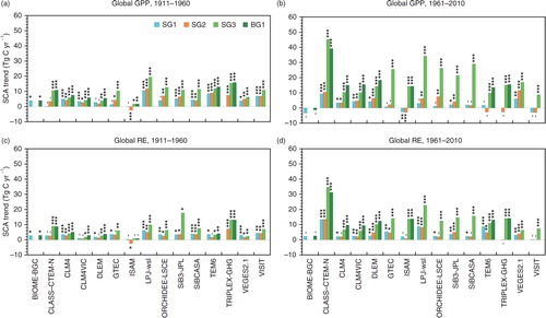
The MsTMIP-model simulations in most cases showed significant increasing trends in the SCA of GPP and RE (Fig. 5). During the period 1911–1960, inter-model differences were not evident, especially for the SG3 and BG1 simulations. During that period, six models (CLM4, CLM4VIC, SiB3, SiBCASA, TEM6 and VISIT) simulated a significant (p<0.001) increasing trend of the SCA of GPP in SG1, for which the simulated variability was driven solely by climate data. During the period 1961–2010, most models simulated more rapid rates of change (i.e. acceleration) of the seasonality of GPP and RE in the SG3 and BG1 simulations. The linear trends of SG3 and BG1 were, in most models, comparable during both periods, the implication being that nitrogen deposition has a small impact on the SCA amplification.

Fig. 5 Linear trends in the SCA of gross fluxes simulated by the MsTMIP models in different periods. (a, b) GPP and (c, d) RE for (a, c) 1911–1960 and (b, d) 1961–2010: ***, p<0.001; **, p<0.01; *, p<0.05; –, insignificant.

The rate of change in the SCA of NEP (cf., Fig. 1b) simulated in the MsTMIP models was smaller in 1911–1960 (Fig. 6) compared with that of GPP and RE, which, because of their similar seasonality, tended to offset each other. Nevertheless, significant increasing trends of the SCA of NEP were found in the simulations of nine models during 1961–2010. In the trends of cumulative NEP amplitude (cf. Fig. 1c), inter-model and inter-simulation differences were a bit clearer (Fig. 6c and d). A few models (SiBCASA, TEM6 and VISIT) showed weak decreasing trends of cumulative NEP seasonality in the SG1 or SG2 simulations, and a majority (11 of 15) of the models evidenced significant increasing trends of NEP seasonality in SG3 simulations.

Fig. 6 Linear trends in the SCA of net fluxes simulated by the MsTMIP models in different periods. (a, b) Monthly NEP and (c, d) cumulative NEP for (a, c) 1911–1960 and (b, d) 1961–2010: ***, p<0.001; **, p<0.01; *, p<0.05; –, insignificant. Result of CLASS-CTEM-N is not shown here, because NEP (= GPP − RE) was always negative.

3.3. Regional difference in SCA trends

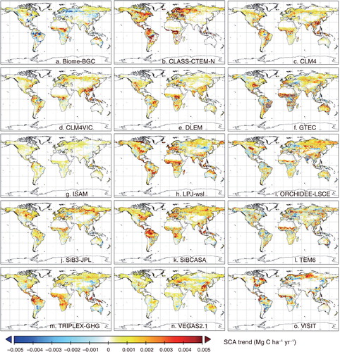
The simulated trends of the SCA showed different spatial distributions among the MsTMIP models, although global total fluxes and their trends were comparable (Fig. 7 for cumulative NEP). Remarkably, a few models (Biome-BGC, GTEC, ORCHIDEE-LSCE and VISIT) showed complicated spatial patterns of decreasing and increasing trends due to different responses to forcing conditions. Several models (CLASS-CTEM-N, GTEC, LPJ-wsl and SiBCASA) simulated amplifying trends in Europe and eastern-central North America, while that were not evident in other models. In the Amazon basin, which is found at low latitudes and undergoes relatively indistinct climate seasonality, the simulated trends were different among the models: amplification in CLASS-CTEM-N, SiBCASA and TRIPLEX-GHG, shrinkage in Biome-BGC and GTEC, and mixed or unclear trends in others. In Siberia, which is located in a boreal region with clear seasonal contrast, five models (GTEC, ORCHIDEE-LSCE, SiB3, SiBCASA and VISIT) showed amplifying trends of seasonality (see Supplementary Fig. 2 for the SCA trends of GPP).

Fig. 7 Distribution of linear trends of the SCA of the cumulative NEP estimated by 15 MsTMIP models during the period 1982–2010 (i.e. comparable to data used in Fig. 10a).

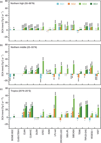
Figure 8 clarifies the latitudinal characteristics (i.e. inter-model and inter-simulation differences) of the simulated trends of the SCA. At high northern latitudes, the majority of the models (11) simulated significant amplification of the cumulative zonal NEP in the SG3 or BG1 simulations, whereas in the Tropics, less than half (6) of the models simulated such amplification. In northern middle latitudes, the majority of the models (10) simulated significant amplification in the SG3 or BG1 simulations. It is remarkable that in the SG1 simulation, four models simulated diminishment of seasonality at northern middle latitudes.

Fig. 8 Linear trends of the SCA of cumulative NEP estimated by MsTMIP models in 1961–2010 for different latitudinal zones. (a) Northern high (55–90°N), northern middle (25–55°N) and tropics (25°N–25°S): ***, p<0.001; **, p<0.01; *, p<0.05; –, insignificant.

4. Discussion

4.1. Global trends of SCA amplification

This study showed that the majority of the contemporary terrestrial ecosystem models simulated amplification of the SCA of atmosphere–ecosystem CO₂ exchange during the experimental period, especially when considering historical climate, land-use and atmospheric CO₂ conditions. Our result is qualitatively consistent with that by Forkel et al. (2016), who showed the dominant contribution of photosynthesis in northern vegetation but used the LPJ-mL model only. Similarly, our result is, at least qualitatively, consistent with the major finding obtained from atmospheric observations (e.g. Graven et al., 2013). The SCA of global mean atmospheric CO₂ concentration (see Supplementary Fig. 1) was 4.40 ppmv during the period 1984–2010; the linear trend of SCA was +0.0122 ppmv yr⁻¹, equivalent to +0.278 % yr⁻¹ and +25.9 Tg C yr⁻¹. These observational value falls within the range of the linear trends of SCA in the cumulative global NEP simulated by the MsTMIP models (Fig. 5d), that is, +41.5±22.9 Tg C yr⁻¹ for SG3 and +32.3±20.0 Tg C yr⁻¹ for BG1. In contrast, the simulated magnitudes of SCA amplification in the SG1 and SG2 scenarios were significantly lower than the observed trend.

The analyses using factorial experimental results were effective to separate the influence of forcing factors on the SCA trends, although there remain uncertainties and inconsistencies with other studies. Indeed, this study could not explain the decrease of the SCA shown by Xu et al. (2013) and Schneising et al. (2014). It is theoretically possible that a reduction in the magnitude or SCA of respiratory CO₂ emissions (sensitive to temperature variability) due to diminished seasonal contrast of temperature resulted in a larger SCA of net ecosystem CO₂ flux (e.g. Gurney and Eckels, 2011; Tian et al., 2015; Yu et al., 2016), if the change in the SCA of GPP did not offset that effect. In this analysis (Fig. 3 and Table 2), both the simulated GPP and RE showed SCA amplification during 1961–2010, and the larger amplification of GPP accounted for the trend of NEP. Moreover, we should be careful about the fact that ecosystem response was different among regions and biomes. For example, winter-green ecosystems (e.g. Mediterranean) would have a different seasonal phase and then different environmental responsiveness from other ecosystems. Also, humid tropical ecosystems may not show clear seasonal patterns, although they respond to interannual climate variability. Therefore, we need more studies to comprehensively account for the trends of the different components of the earth system.

It has also been difficult to separate the photosynthetic enhancement (Figs. 3 and 4) into contributions from canopy-level LAI expansion (i.e. structural response) and increased leaf-level gas exchange (i.e. physiological response). Figure 9a shows the relationship between the trend of LAI and the trend in GPP for each model simulation. In the SG1 and SG2 scenarios, the LAI trend was weak and the relationship between the trends was unclear, and the implication being that the moderate amplification in these simulations was largely attributable to a physiological response. In contrast, many SG3-model simulations showed a considerable increase in LAI seasonality and a corresponding trend of amplification of GPP seasonality. This result implies that in these model simulations, a structural response in combination with a physiological response accounted for the larger magnitude of the SCA amplification. This finding is consistent with the satellite-observed SCA trend of northern vegetation LAI in recent decades (Jeganathan et al., 2014).

Fig. 9 Relationship between the SCA metrics and carbon budget metrics. Results of the northern middle latitude (25–55°N) in 1961–2010 for SG1, SG2 and SG3 simulations are shown. (a) Relationship between the trend of the SCA of leaf area index (LAI, model estimation) and the trend of the SCA of monthly GPP. (b) Relationship between the trend of the SCA of cumulative NEP and accumulated carbon uptake during the period.

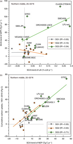
Another interesting question is whether such seasonal amplification is related to the strength of carbon uptake by terrestrial ecosystems. Because SCA is likely to indicate overall activity of atmosphere–ecosystem CO₂ exchange, we may hypothesize that the SCA is related to ecosystem fluxes, particularly net carbon uptake, for a certain period. Fig. 9b shows that the simulated linear trend of the SCA of NEP in northern middle latitude is well correlated with net terrestrial carbon sequestration during 1961–2010 in the SG1 to SG3 simulations. This result is remarkable, because Zhao and Zeng (2014) found a similar relationship by using a different data set of future projections from the Climate Model Intercomparison Project. Furthermore, it is remarkable that the relationship in this study was obtained as an aggregated result of multiple terrestrial model simulations, and it implies that monitoring of seasonality has implications for long-term carbon uptake.

4.2. Human impacts on SCA amplification

In this study, the MsTMIP-based analyses implied that human activities exerted influences on the SCA of terrestrial CO₂ fluxes. Several recent studies (Gray et al., 2014; Zeng et al., 2014) have proposed that growth of agricultural production during the last decades accounts, at least in part, for the observed amplification of atmospheric CO₂ seasonality. In our study, the influence of land-use change, including cropland conversion, was evident in the difference between the SG1 and SG2 results and explained on average 17.8 % of the combined amplification in SG3. The magnitude of this effect is smaller than the approximate 45 % amplification estimated by Zeng et al. (2014), who used the VEGAS model to take account of historical changes in agricultural management. In their paper, they implied that the Green Revolution played an important role in the augmentation of the SCA after the 1950s. The results of the present analysis showed a consistent acceleration of the amplification of the SCA (Figs. 3 and 5), although there remain uncertainties about the precise magnitude.

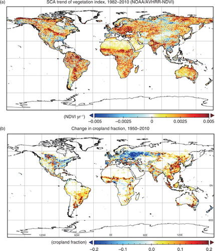
A time-series of a satellite-observed vegetation index (Fig. 10a) shows amplification of the SCA over large areas of land, especially in central North America, South America, Central to Eastern Europe, the Sahel, India, eastern Siberia and eastern Australia. Many of these regions overlap regions where the fraction of cropland has increased during the past several decades (Fig. 10b). Many models simulated such SCA amplification in cultivated regions (Fig. 7), although there was not a high degree of confidence in data for cultivated areas. For example, amplification in central North America was clearly simulated by GTEC, LPJ-wsl, ORCHIDEE-LSCE and SiBCASA. In contrast, increased cultivation in East Asia was unrelated to seasonal-cycle amplification of the vegetation index, and the models showed inconsistent results. Additionally, the modern change of the cropland fraction (Fig. 10b) showed a broad area of decrease in Eastern Europe. This decrease was perhaps attributable to cropland abandonment after the Chernobyl nuclear power accident in the Ukraine in April 1986. In many of these areas of cropland decrease, the SCA of the vegetation index was enhanced, but for undefined reasons (e.g. regrowth of natural vegetation).

Fig. 10 (a) Distribution of the linear trend of the SCA (i.e. max–min difference) of the Normalized Difference Vegetation Index (NDVI) in 1982–2010, and (b) distribution of the change in cropland fraction 1950–2010 obtained from the data set by Hurtt et al. (2011).

4.3. Missing factors and future direction

Our study provided an analysis consistent with a decadal-scale amplification of the SCA in atmosphere–ecosystem CO₂ exchange. It is important to note that considerable uncertainties remain in the present model simulations. The present study used 15-model results to derive less biased conclusions concerning the trend of the SCA, but this strategy does not guarantee that inter-model disparity represents the full range of estimation uncertainty or that the mean or median of these model results is necessarily the most accurate. For example, several process-oriented studies (e.g. Richardson et al., 2012; Alexandrov, 2014) have revealed that present terrestrial models are insufficient to capture seasonal phenomena such as leaf phenology and substrate limitation. Although many contemporary models consistently simulated such amplification, this study has some shortcomings, as discussed below.

Several studies (e.g. van der Werf et al., 2010) have indicated that biomass burning has clear seasonal variability; that is, larger combustion emissions occur in the northern summer. The result is leading to larger seasonality of terrestrial emissions and an offset of photosynthetic uptake. Only a limited number of MsTMIP models explicitly take account of fire-induced carbon emissions (and the following recovery of vegetation): Biome-BGC, CLM, CLM4VIC, DLEM, LPJ and VEGAS. To avoid inconsistency in the definition of net CO₂ flux, this study defined NEP as the difference between photosynthesis and respiration [cf., eq. (1)] for all the models. This definition made the present analyses clearer, but we still need to account for the impact of biomass burning when interpreting the temporal trend in atmospheric CO₂ seasonality. Mouillot et al. (2006) showed that global emissions from biomass burning have gradually increased in the twentieth century, especially in tropical forests and tropical savannas. Yang et al. (2015) found a significant declining trend in global pyrogenic carbon emissions between the early twentieth century and the mid-1980s but a significant upward trend between the mid-1980s and the 2000s as a result of more frequent fires in ecosystems with high carbon storage, such as peatlands and tropical forests. Also, Zimov et al. (1999) stated that disturbed ecosystems have larger SCAs than undisturbed ones, because of increased uptake in summer and increased release in winter. It is noteworthy, especially when comparing with atmospheric data, that anthropogenic CO₂ emission from fossil fuel combustion has an opposite seasonal phase (i.e. peak in winter) and has been increased during the last decades (e.g. Andres et al., 2011). This emission increase could partly contribute to the amplification of atmospheric CO₂ seasonality. Apparently, we need more studies to clarify the roles of disturbance and human activity in altering the SCA.

In many models, agricultural management was included, but in quite a simplified manner. It is still difficult for terrestrial models to take account of actual management practices such as irrigation, tillage, multi-cropping and crop rotation, which could affect the magnitude and seasonality of CO₂ exchange over croplands. A few studies have provided global, spatially explicit crop calendar data with respect to planting and harvest dates (e.g. Sacks et al., 2010) but only for the present time. To account for historical changes in agricultural management and its impact, we need to develop a general and practical scheme of agricultural practices.

4.4. Implications for observations and future projection

The seasonality of terrestrial ecosystems has focused attention on observations of the responses of vegetation to global environmental change. For example, the timing of leaf display and shedding of deciduous-type vegetation is responsive to interannual changes of temperature and therefore is useful for monitoring the functional properties of vegetation (e.g. Gunderson et al., 2012; Keenan et al., 2014). Recently, Buitenwerf et al. (2015) and Fu et al. (2015) have analysed worldwide leaf phenology data and have indicated that the impact of phenological changes on ecosystem functions differs among regions and varies through time. Such monitoring has also been conducted by means of satellite remote sensing, which now provides up to 30 yr of global data (e.g. Zhu et al., 2013). In addition to monitoring by optical images, flux measurements by the eddy covariance method have been providing novel and rigorous evidence about terrestrial ecosystem functions, including their seasonality. For example, Piao et al. (2008) have shown that in northern ecosystems, autumn warming would result in increases of net carbon release as a result of enhanced respiratory emissions. Several studies (e.g. Angert et al., 2005; Buermann et al., 2013) showed that there would be trade-offs between seasonal responses of vegetation to temperature change, for example, earlier spring onset accompanied with weaker summer uptake. Such seasonal changes in responsiveness may be more complicated than is presently known, and thus, observations of the seasonality of vegetation (e.g. amplitude and phase) are expected to provide in-depth knowledge about ecosystem functional properties.

Our study also indicated that monitoring of ecosystem seasonality would provide useful insights concerning ecosystem dynamics. The clear relationship between the amplification trend and net carbon uptake (Fig. 9b) suggests that observations of seasonality have implications for long-term functionality. In a near-stationary state, the SCA may be independent of annual net carbon uptake, which is expected to be near zero. However, during a monotonic environmental change such as an atmospheric CO₂ rise, amplification of the seasonal activity of vegetation may be accompanied by an increase in annual carbon assimilation and can then be related to net ecosystem carbon uptake. However, it should be aware of that there can be other possibility that the SCA trend of NEP is caused by different (perhaps independent) mechanisms such as a change in winter respiration (Tian et al., 2015). Examining the hypothesis by in situ observations is an essential task, but it requires a few decades of continuous monitoring. A few long-term measurements may allow us to address this issue. For example, Urbanski et al. (2007) analysed long-term flux data at the Harvard Forest and showed that the strength of annual net carbon uptake had increased for more than 13 yr. Remarkably, the increase in annual carbon uptake was accompanied by an expansion of the differences between GPP and RE and between growing and dormant periods, the implication in both cases being an amplification of the SCA in the forest. In the case of Arctic ecosystems, Belshe et al. (2013) has conducted a meta-analysis across 54 observational studies and has shown that growing-season net CO₂ uptake has generally increased since the 1990s. They also showed that an increase in dormant-season CO₂ release has led to an increase in CO₂ release from tundra ecosystems. Thus, the fact that the relationship between seasonality and the annual total carbon budget seems subject to change should encourage further observations to derive general tendencies with higher confidence.

Finally, we emphasize here again that model intercomparison, especially in conjunction with factorial experiments, is one of the most practical and effective research approaches to perform a rigorous analysis of global and regional carbon exchanges and their seasonality. These model-based outcomes should be examined and combined with observational evidence to achieve knowledge that is less biased. With respect to the SCA amplification issue, it is an interesting task to simulate spatial and temporal patterns of atmospheric CO₂ concentrations using multiple terrestrial fluxes (e.g. MsTMIP data) combined with atmospheric transport models (e.g. TransCom; Law et al., 2008). Additional sensitivity simulations aimed at separating the impacts of these meteorological variables would provide further insights into ecosystem responsiveness to environmental change. Through these efforts, more insights into terrestrial ecosystem functions under changing global environments should be possible. Those insights should improve the credibility of models for making future climate projections using Earth system models, in which terrestrial ecosystem models are embedded.

5. Acknowledgements

Funding for the Multi-scale synthesis and Terrestrial Model Intercomparison Project (MsTMIP; www.nacp.ornl.gov/MsTMIP.shtm) activity was provided through NASA ROSES Grant #NNX10AG01A. Data management support for preparing, documenting and distributing model driver and output data was performed by the Modeling and Synthesis Thematic Data Center at Oak Ridge National Laboratory (ORNL; www.nacp.ornl.gov), with funding through NASA ROSES Grant #NNH10AN681. Finalized MsTMIP data products are archived at the ORNL DAAC (www.daac.ornl.gov).

Biome-BGC code was provided by the Numerical Terradynamic Simulation Group at University of Montant. The computational facilities were provided by NASA Earth Exchange at NASA Ames Research Center.

CLASS-CTEM-N+: CLASS and CTEM models were originally developed by the Climate Research Branch and Canadian Centre for Climate Modelling and Analysis (CCCMa) of Environment Canada, respectively. MsTMIP related work was funded by the Natural Sciences and Engineering Research Council (NSERC) grants. Computational support was provided by the SHARCNET.

CLM4 research is supported in part by the US Department of Energy (DOE), Office of Science, Biological and Environmental Research. Oak Ridge National Laboratory is managed by UT-BATTELLE for DOE under contract DE-AC05-00OR22725.

CLM4VIC simulations were supported in part by the U.S. DOE, Office of Science, Biological and Environmental Research (BER) through the Earth System Modeling program and performed using the Environmental Molecular Sciences Laboratory (EMSL), a national scientific user facility sponsored by the U.S.DOE-BER and located at Pacific Northwest National Laboratory (PNNL). Participation of M. Huang in the MsTMIP synthesis is supported by the U.S.DOE-BER through the Subsurface Biogeochemical Research Program (SBR) as part of the SBR Scientific Focus Area (SFA) at the Pacific Northwest National Laboratory (PNNL). PNNL is operated for the U.S. DOE by BATTELLE Memorial Institute under contract DE-AC05-76RLO1830.

DLEM developed in International Center for Climate and Global Change Research, Auburn University, has been supported by NASA grants (NNX11AD47G; NNX14AF93G, NNX08AL73G, NNX14AO73G, NNX10AU06G, NNG04GM39C), NSF grants (AGS-1243232, AGS-1243220, CNH-1210360), US DOE National Institute for Climate Change Research (DUKE-UN-07-SC-NICCR-1014) and US EPA STAR program (2004-STAR-L1).

LPJ-wsl work was conducted at LSCE, France, using a modified version of LPJ version 3.1 model, originally made available by the Potsdam Institute for Climate Impact Research.

ORCHIDEE is a global land surface model developed at the IPSL institute in France. The simulations were performed with the support of the GhG Europe FP7 grant with computing facilities provided by ‘LSCE’ or ‘TGCC’.

SiB3-JPL research was carried out at the Jet Propulsion Laboratory, California Institute of Technology, under a contract with the National Aeronautics and Space Administration.

TEM6 research is supported in part by the US DOE, Office of Science, Biological and Environmental Research.

TRIPLEX-GHG was developed at University of Quebec at Montreal (Canada) and Northwest A&F University (China) and has been supported by the National Basic Research Program of China (2013CB956602) and the National Science and Engineering Research Council of Canada (NSERC) Discover Grant.

VISIT was developed at the National Institute of Environmental Studies, Japan. This work was mostly conducted during an extended visit to Oak Ridge National Laboratory.

This study was supported by KAKENHI Grant No. 26281014 by the Japan Society for the Promotion of Science.

Notes

To access the supplementary material to this article, please see Supplementary files under ‘Article Tools’.

References

- Alexandrov G. A . Explaining the seasonal cycle of the globally averaged CO2 with a carbon-cycle model. Earth Syst. Dynam. 2014; 5: 345–354.
- Andres R. J. , Gregg J. S. , Losey L. , Marland G. , Boden T. A . Monthly, global emissions of carbon dioxide from fossil fuel consumption. Tellus B. 2011; 63: 309–327.
- Angert A. , Biraud S. , Bonfils C. , Henning C. C. , Buermann W , co-authors . Drier summers cancel out the CO2 uptake enhancement induced by warmer springs. Proc. Natl. Acad. Sci. 2005; 102: 10823–10827.
- Bacastow R. B. , Keeling C. D. , Whorf T. P . Seasonal amplitude increase in atmospheric CO2 concentration at Mauna Loa, Hawaii, 1959–1982. J. Geophys. Res. 1985; 90: 10529–10540.
- Baker I. T., Prihodko L., Denning A. S., Goulden M., Miller S., co-authors. Seasonal drought stress in the Amazon: reconciling models and observations. J. Geophys. Res. 2008; 113 G00B01. DOI: http://dx.doi.org/10.1029/2007JG000644.
- Baldocchi D. , Falge E. , Gu L. , Olson R. , Hollinger D. , co-authors . FLUXNET: a new tool to study the temporal and spatial variability of ecosystem-scale carbon dioxide, water vapor, and energy flux densities. Bull. Am. Meteorol. Soc. 2001; 82: 2415–2434.
- Barichivich J. , Briffa K. R. , Myneni R. B. , Osborn T. J. , Melvin T. M. , co-authors . Large-scale variations in the vegetation growing season and annual cycle of atmospheric CO2 at high northern latitudes from 1950–2011. Global Change. Biol. 2013; 19: 3167–3183.
- Belshe E. F. , Schuur E. A. G. , Bolker B. M . Tundra ecosystems observed to be CO2 sources due to differential amplification of the carbon cycle. Ecol. Lett. 2013; 16: 1307–1315.
- Buermann W., Bikash P. R., Jung M., Burn D. H., Reichstein M. Earlier springs decrease peak summer productivity in North American boreal forests. Environ. Res. Lett. 2013; 8 DOI: http://dx.doi.org/10.1088/1748-9326/1088/1082/024027.
- Buitenwerf R. , Rose L. , Higgins S. I . Three decades of multi-dimensional change in global leaf phenology. Nat. Clim. Change. 2015; 5: 364–368.
- Cramer W. , Kicklighter D. W. , Bondeau A. , Moore B. I. , Churkina G. , co-authors . Comparing global NPP models of terrestrial net primary productivity (NPP): overview and key results. Global Change Biol. 1999; 5: 1–15.
- Forkel M. , Carvalhais N. , Rödenbeck C. , Keeling R. , Heimann M. , co-authors . Enhanced seasonal CO2 exchange caused by amplified plant productivity in northern ecosystems. Science. 2016; 351: 696–699.
- Fu Y. H. , Zhao H. , Piao S. , Peaucelle M. , Peng S. , co-authors . Declining global warming effects on the phenology of spring leaf unfolding. Nature. 2015; 526: 104–107.
- Graven H. D. , Keeling R. F. , Piper S. C. , Patra P. K. , Stephens B. B. , co-authors . Enhanced seasonal exchange of CO2 by northern ecosystems since 1960. Science. 2013; 341: 1085–1089.
- Gray J. M. , Frolking S. , Kort E. A. , Ray D. K. , Kucharik C. J. , co-authors . Direct human influence on atmospheric CO2 seasonality from increased cropland productivity. Nature. 2014; 515: 398–401.
- Gunderson C. A. , Edwards N. T. , Walker A. V. , O'Hara K. H. , Campion C. M. , co-authors . Forest phenology and a warmer climate – growing season extension in relation to climatic provenance. Global Change. Biol. 2012; 18: 2008–2025.
- Gurney K. R. , Eckels W. J . Regional trends in terrestrial carbon exchange and their seasonal signatures. Tellus B. 2011; 63: 328–339.
- Hayes D. J., McGuire A. D., Kicklighter D. W., Gurney K. R., Burnside T. J., co-authors. Is the northern high-latitude land-based CO2 sink weakening?. Global Biogeochem. Cycles. 2011; 25 GB3018. DOI: http://dx.doi.org/10.1029/2010GB003813.
- Huang S. , Arain M. A. , Arora V. K. , Yuan F. , Brodeur J. , co-authors . Analysis of nitrogen controls on carbon and water exchanges in a conifer forest using the CLASS-CTEM N+ model. Ecol. Model. 2011; 222: 3743–3760.
- Huntzinger D. N. , Schwalm C. , Michalak A. M. , Schaefer K. , King A. W. , co-authors . The North American Carbon Program Multi-scale Synthesis and Terrestrial Model Intercomparison Project: Part 1: overview and experimental design. Geosci. Model Dev. 2013; 6: 2121–2133.
- Hurtt G. C. , Chini L. P. , Frolking S. , Betts R. A. , Feddema J. , co-authors . Harmonization of land-use scenarios for the period 1500–2100: 600 years of global gridded annual land-use transitions, wood harvest, and resulting secondary lands. Clim. Change. 2011; 109: 117–161.
- Ito A. , Inatomi M . Water-use efficiency of the terrestrial biosphere: a model analysis on interactions between the global carbon and water cycles. J. Hydrometeorol. 2012; 13: 681–694.
- Jain A. K., Yang X. Modeling the effects of two different land cover change data sets on the carbon stocks of plants and soils in concert with CO2 and climate change. Global. Biogeochem. Cycles. 2005; 19 GB2015. DOI: http://dx.doi.org/10.1029/2004GB002349.
- Jeganathan C. , Dash J. , Atkinson P. M . Remotely sensed trends in the phenology of northern high latitude terrestrial vegetation, controlling for land cover change and vegetation type. Remote Sens. Environ. 2014; 143: 154–170.
- Jung M., Reichstein M., Margolis H. A., Cescatti A., Richardson A. D., co-authors. Global patterns of land-atmosphere fluxes of carbon dioxide, latent heat, and sensible heat derived from eddy covariance, satellite, and meteorological observations. J. Geophys. Res. 2011; 116 G00J07. DOI: http://dx.doi.org/10.1029/2010JG001566.
- Keeling C. D. , Chin J. F. S. , Whorf T. P . Increased activity of northern vegetation inferred from atmospheric CO2 measurements. Nature. 1996; 382: 146–149.
- Keenan T. F. , Gray J. , Friedl M. A. , Toomey M. , Bohrer G. , co-authors . Net carbon uptake has increased through warming-induced changes in temperate forest phenology. Nat. Clim. Change. 2014; 4: 598–604.
- Kohlmaier G. H. , Sire E.-O. , Janecek A. , Keeling C. D. , Piper S. C. , co-authors . Modelling the seasonal contribution of a CO2 fertilization effect of the terrestrial vegetation to the amplitude increase in atmospheric CO2 at Mauna Loa Observatory. Tellus B. 1989; 41: 487–510.
- Krinner G., Viovy N., de Noblet-Ducoudré N., Ogée J., Polcher J., co-authors. A dynamic global vegetation model for studies of the coupled atmosphere-biosphere system. Global Biogeochem. Cycles. 2005; 19 GB1015. DOI: http://dx.doi.org/10.1029/2003GB002199.
- Law R. M., Peters W., Rödenbeck C., Aulagnier C., Baker I., co-authors. TransCom model simulations of hourly atmospheric CO2: experimental overview and diurnal cycle results for 2002. Global Biogeochem. Cycles. 2008; 22 GB3009. DOI: http://dx.doi.org/10.1029/2007GB003050.
- Lei H. , Huang M. , Leung L. R. , Yang D. , Shi X. , co-authors . Sensitivity of global terrestrial gross primary production to hydrologic states simulated by the community land model using two runoff parameterizations. J. Adv. Model Earth Syst. 2014; 6: 658–679.
- Le Quéré C. , Moriarty R. , Andrew R. M. , Canadell J. G. , Sitch S. , co-authors . Global carbon budget 2015. Earth Syst. Sci. Data. 2015; 7: 349–396.
- Luo Y. , Keenan T. F. , Smith M . Predictability of the terrestrial carbon cycle. Global Change Biol. 2015; 27: 1737–1751.
- Mao J. , Thornton P. E. , Shi X. , Zhao M. , Post W. M . Remote sensing evaluation of CLM4 GPP for the period 2000–09. J. Clim. 2012; 25: 5327–5342.
- Mouillot F., Narasimha A., Balkanski Y., Lamarque J.-F., Field C. B. Global carbon emissions from biomass burning in the 20th century. Geophys. Res. Lett. 2006; 33 L01801. DOI: http://dx.doi.org/10.1029/2005GL024707.
- Myneni R. B. , Keeling C. D. , Tucker C. J. , Asrar G. , Nemani R. R . Increased plant growth in the northern high latitudes from 1981 to 1991. Nature. 1997; 386: 698–702.
- Peng S., Ciais P., Chevallier F., Peylin P., Cadule P., co-authors. Benchmarking the seasonal cycle of CO2 fluxes simulated by terrestrial ecosystem models. Global Biogeochem. Cycles. 2015; 29: 46–64. DOI: http://dx.doi.org/10.1002/2014GB004931.
- Piao S., Ciais P., Friedlingstein P., de Noblet-Ducoudré N., Cadule P., co-authors. Spatiotemporal patterns of terrestrial carbon cycle during the 20th century. Global Biogeochem. Cycles. 2009; 23 GB4026. DOI: http://dx.doi.org/10.1029/2008GB003339.
- Piao S. , Ciais P. , Friedlingstein P. , Peylin P. , Reichstein M. , co-authors . Net carbon dioxide losses of northern ecosystems in response to autumn warming. Nature. 2008; 451: 49–52.
- Post W. M. , King A. W. , Wullschleger S. D . Historical variations in terrestrial biospheric carbon storage. Global Biogeochem. Cycles. 1997; 11: 99–109.
- Randerson J. T. , Thompson M. V. , Conway T. J. , Fung I. Y. , Field C. B . The contribution of terrestrial sources and sinks to trends in the seasonal cycle of atmospheric carbon dioxide. Global Biogeochem. Cycles. 1997; 11: 535–560.
- Ricciuto D. M., King A. W., Dragoni D., Post W. M. Parameter and prediction uncertainty in an optimized terrestrial carbon cycle model: effects of constraining variables and data record length. J. Geophys. Res. 2011; 116 G01033. DOI: http://dx.doi.org/10.1029/2010JG001400.
- Richardson A. D. , Anderson R. S. , Arain M. A. , Barr A. G. , Bohrer G. , co-authors . Terrestrial biosphere models need better representation of vegetation phenology: results from the North American Carbon Program Site Synthesis. Global Change Biol. 2012; 18: 566–584.
- Richardson A. D. , Keenan T. F. , Migliavacca M. , Ryu Y. , Sonnentag O. , co-authors . Climate change, phenology, and phenological control of vegetation feedbacks to the climate system. Agric. For. Meteorol. 2013; 169: 156–173.
- Sacks W. J. , Deryng D. , Foley J. A. , Ramankutty N . Crop planting dates: an analysis of global patterns. Global Ecol. Biogeogr. 2010; 19: 607–620.
- Schaefer K., Collatz G. J., Tans P., Denning A. S., Baker I., co-authors. Combined Simple Biosphere/Carnegie-Ames-Stanford Approach terrestrial carbon cycle model. J. Geophys. Res. 2008; 113 G03034. DOI: http://dx.doi.org/10.1029/2007JG000603.
- Schimel D. , Stephens B. B. , Fisher J. B . Effect of increasing CO2 on the terrestrial carbon cycle. Proc. Natl. Acad. Sci. 2015; 112: 436–441.
- Schneising O. , Reuter M. , Buchwitz M. , Heymann J. , Bovensmann H. , co-authors . Terrestrial carbon sink observed from space: variation of growth rates and seasonal cycle amplitudes in response to interannual surface temperature variability. Atmos. Chem. Phys. 2014; 14: 133–141.
- Shi X., Mao J., Thornton P. E., Hoffman F. M., Post W. M. The impact of climate, CO2, nitrogen deposition and land use change on simulated contemporary global river flow. Geophys. Res. Lett. 2011; 38 L08704. DOI: http://dx.doi.org/10.1029/2011GL046773.
- Sitch S. , Huntingford C. , Gedney N. , Levy P. E. , Lomas M. , co-authors . Evaluation of the terrestrial carbon cycle, future plant geography and climate – carbon cycle feedbacks using five Dynamic Global Vegetation Models (DGVMs). Global Change Biol. 2008; 14: 2015–2039.
- Sitch S. , Smith B. , Prentice I. C. , Arneth A. , Bondeau A. , co-authors . Evaluation of ecosystem dynamics, plant geography and terrestrial carbon cycling in the LPJ dynamic global vegetation model. Global Change Biol. 2003; 9: 161–185.
- Thornton P. E. , Law B. E. , Gholz H. L. , Clark K. L. , Falge E. , co-authors . Modeling and measuring the effects of disturbance history and climate on carbon and water budgets in evergreen needle leaf forests. Agric. For. Meteorol. 2002; 113: 185–222.
- Tian H. , Chen G. , Zhang C. , Liu M. , Sun G. , co-authors . Century-scale responses of ecosystem carbon storage and flux to multiple environmental changes in the southern United States. Ecosystems. 2012; 15: 674–694.
- Tian H., Lu C., Yang J., Banger K., Huntzinger D. N., co-authors. Global patterns and controls of soil organic carbon dynamics as simulated by multiple terrestrial biosphere models: current status and future directions. Global Biogeochem. Cycles. 2015; 29 DOI: http://dx.doi.org/10.1002/2014GB005021.
- Tian H., Xu X., Lu C., Liu M., Ren W., co-authors. Net exchanges of CO2, CH4, and N2O between China's terrestrial ecosystems and the atmosphere and their contributions to global climate warming. J. Geophys. Res. 2011; 116 G02011. DOI: http://dx.doi.org/10.1029/2010JG001393.
- Urbanski S., Barford C., Wofsy S., Kucharik C., Pyle E., co-authors. Factors controlling CO2 exchange on timescales from hourly to decadal at Harvard Forest. J. Geophys. Res. 2007; 112 G02020. DOI: http://dx.doi.org/10.1029/2006JG000293.
- van der Werf G. R. , Randerson J. T. , Giglio L. , Collatz G. J. , Mu M. , co-authors . Global fire emissions and the contribution of deforestation, savanna, forest, agricultural, and peat fires (1997–2009). Atmos. Chem. Phys. 2010; 10: 11707–11735.
- Wei Y. , Liu S. , Huntzinger D. N. , Michalak A. M. , Viovy N. , co-authors . The North American Carbon Program Multipscale Synthesis and Terrestrial Model Intercomparison Project – Part 2: environmental driver data. Geosci. Model Dev. 2014; 7: 2875–2893.
- Xu L. , Myneni R. B. , Chapin F. S. I. , Callaghan T. V. , Pinzon J. E. , co-authors . Temperature and vegetation seasonality diminishment over northern lands. Nat. Clim. Change. 2013; 3: 581–586.
- Yang J., Tian H., Tao B., Ren W., Lu C., co-authors. Century-scale patterns and trends of global pyrogenic carbon emissions and fire influences on terrestrial carbon balance. Global Biogeochem. Cycles. 2015; 29 DOI: http://dx.doi.org/10.1002/2015GB005160.
- Yu Z., Wang J., Liu S., Piao S., Ciais P., co-authors. Decrease in winter respiration explains 25% of the annual northern forest carbon sink enhancement over the last 30 years. Global Ecol. Biogeogr. 2016; 25: 586–595. DOI: http://dx.doi.org/10.1111/geb.12441.
- Zeng N., Mariotti A., Wetzel P. Terrestrial mechanisms of interannual CO2 variability. Global Biogeochem. Cycles. 2005; 19 GB1016. DOI: http://dx.doi.org/10.1029/2004GB002273.
- Zeng N. , Zhao F. , Collatz G. J. , Kalnay E. , Salawitch R. J. , co-authors . Agricultural Green Revolution as a driver of increasing atmospheric CO2 seasonal amplitude. Nature. 2014; 515: 394–397.
- Zhang K., Kimball J. S., Hogg E. H., Zhao M., Oechel W. C., co-authors. Satellite-based model detection of recent climate-driven changes in northern high-latitude vegetation productivity. J. Geophys. Res. 2008; 113 G03033. DOI: http://dx.doi.org/10.1029/2007JG000621.
- Zhao F. , Zeng N . Continued increase in atmospheric CO2 seasonal amplitude in the 21st century projects by the CMIP5 Earth system models. Earth Syst. Dynam. 2014; 5: 423–439.
- Zhu Q. , Liu J. , Peng C. , Chen H. , Fang X. , co-authors . Modelling methane emissions from natural wetlands by development and application of the TRIPLEX-GHG model. Geosci. Model Dev. 2014; 7: 981–999.
- Zhu Z. , Bi J. , Pan Y. , Ganguly S. , Anav A. , co-authors . Global data sets of vegetation leaf area index (LAI)3g and fraction of photosynthetically active radiation (FPAR)3g derived from Global Inventory Modeling and Mapping Studies (GIMMS) Normalized Difference Vegetation Index (NDVI3g) for the period 1981 to 2011. Remote Sens. 2013; 5: 927–948.
- Zimov S. A. , Davidov S. P. , Zimova G. M. , Davidova A. I. , Chapin F. S. III. , co-authors . Contribution of disturbance to increasing seasonal amplitude of atmospheric CO2 . Science. 1999; 284: 1973–1977.
- Zscheischler J. , Michalak A. M. , Schwalm C. , Mahecha M. D. , Huntzinger D. N. , co-authors . Impact of large-scale climate extremes on biospheric carbon fluxes: an imtercomparison based on MsTMIP data. Global Biogeochem. Cycles. 2014; 28: 585–600.