Horizontal scales of ice-supersaturated regions

Abstract

Ice-supersaturated regions (ISSRs) as seen from routine measurements onboard commercial long-distance aircrafts are investigated. We use data in the time interval 1995–1999 for investigating properties of ISSRs as pathlengths and distances between ISSRs. Additionally, the horizontal separation of ISSRs and the gradients of relative humidity over ice at the edges of ISSRs are evaluated. Here, we concentrate on the representation of large-scale features of ISSRs vs. small-scale variations. We additionally use idealised simulations for investigating the connection between small-scale relative humidity variations and variability on larger scales.

• ice supersaturation
• multiple scales
• ice clouds

1. Introduction

The existence of air masses in the status of supersaturation with respect to ice was conjectured more than 100 years ago by Wegener (1911). In fact, about 60 years ago, measurements in the tropopause region could corroborate this conjecture (Glückauf, 1945). In the last 25 years, in situ measurements of ice supersaturation in the upper troposphere and lower stratosphere (UTLS) could be obtained by a huge variety of measurement techniques (e.g. Helten et al., 1998; Jensen et al., 1998; Zöger et al., 1999; Ovarlez et al., 2000; Zondlo et al., 2010). These measurements show that air masses in the status of ice supersaturation, so-called ice-supersaturated regions (ISSRs, see, e.g., Gierens et al., 1999), occur quite frequently in the tropopause region. ISSRs are an interesting research topic for several reasons. Cloud-free ISSRs are potential formation regions for natural and anthropogenic ice clouds (cirrus clouds and contrails, respectively) and ice supersaturation is very common in pure ice clouds (see, e.g., Krämer et al., 2009). In the low temperature regime, two major pathways for ice crystal formation are possible, namely heterogeneous nucleation (involving solid aerosol particles; see, e.g., Hoose and Möhler, 2012), and homogeneous freezing of solution droplets (Koop et al., 2000). For both formation pathways, high values of ice supersaturation are required. The formation of contrails is determined by the Schmidt–Appleman criterion (Schmidt, 1941; Appleman, 1953; Schumann, 1996), which is mostly dependent on temperature. However, for a persistent contrail (i.e. life times longer than 2 minutes), ice supersaturation is required; otherwise, ice crystals would sublimate in the subsaturated air. Ice clouds are, as all other clouds, important regulators of Earth's energy budget. They scatter incoming solar radiation back to space (albedo effect) and trap terrestrial infrared radiation (greenhouse effect). In contrast to other clouds, the net effect of natural cirrus clouds is not known yet. In fact, even the sign of the effect is uncertain, although a net warming is often assumed (Chen et al., 2000). For contrails, a net warming has been derived in earlier studies (Sausen et al., 2005; Stuber and Forster, 2007). Besides the implications for ice cloud formation and evolution, ice supersaturation itself constitutes an interesting topic in atmospheric physics; obviously, large parts in the UTLS are in a thermodynamic state far away from equilibrium. From non-equilibrium thermodynamics, it is well known that such systems enforce pattern formation and instabilities (e.g. Nicolis and Prigogine, 1977). Therefore, we have at least two good reasons for investigating ice supersaturation in the tropopause region.

The origin of ISSRs in the UTLS is not clear. From a theoretical point of view we can inspect relative humidity with respect to ice:1

where T, p denote temperature and pressure, q is specific humidity (mass water vapour per mass dry air), ε is the ratio of molar masses of water and air, and p _si (T) denotes saturation pressure over ice, respectively. If we investigate the total derivative of relative humidity with respect to ice,2

it is quite clear that RHi can increase due to (a) decrease in temperature (dT<0), (b) increase in pressure (dp>0) and (c) increase in specific humidity (dq>0). For the increase of RHi, we investigate two special cases, i.e. (a) adiabatic expansion (dT<0, dp<0) and (b) general increase of specific humidity under isothermal/isobaric conditions (dq>0).

For vertical upward motions in the atmosphere, we usually assume adiabatic processes, i.e. the relative humidity will increase due to decreasing temperature and pressure; in fact, the impact of temperature is usually dominant, whereas pressure changes are higher order effects, which would slightly compensate the increase in RHi. If an isolated air parcel is investigated, there is also transport of water vapour. Whereas temperature and pressure is changed, we can assume that the mass of water vapour inside the parcel remains constant (neglecting mixing with the environment). Thus, water vapour from warmer/moister layers below is lifted to a higher level. The water vapour mixing ratio could also be changed. The only relevant process for changing water vapour mass concentration without cloud processes is mixing of an air parcel with environmental air. For instance, this process occurs in case of contrail formation. Warm and moist aircraft exhaust mixes with cold and dry air, leading to supersaturation with respect to water. Then, water droplets are formed, which in turn freeze due to cold temperatures, resulting from mixing of warm exhaust and cold environmental air. Mixing might also occur for (ascending) air parcels, which are brought into an environment resulting in large gradients in water vapour concentrations (air parcel vs. environmental air). Convection might also lead to mixing (see, e.g. Spichtinger, 2014). For regimes dominated by large-scale motions without strong dynamics on cloud scales, we can assume that mixing is quite small and in terms of the parcel view adiabatic processes are dominant.

Satellite measurements indicate that the frequency of occurrence of ISSRs is enhanced for extratropics in the regions of enhanced storm activity, i.e. in the storm tracks (Spichtinger et al., 2003b; Gettelman et al., 2006). Thus, we assume that large-scale dynamics should influence the formation and evolution of ice supersaturation in the tropopause region in a dominant way. Synoptic weather features as fronts or warm conveyor belts associated with low pressure systems lead to synoptic upward motions in the order of a few centimetres per seconds (typical values w~3 − 8 cm s⁻¹).

In the tropics, frequency of occurrence for ISSRs is enhanced for regions with dominant deep convection. Layers on top of developing convection experience moderate updrafts leading to ice supersaturation. The occurrence of subvisible cirrus in the tropics points to this formation mechanism (Gierens et al., 2000; Jensen and Ackerman, 2006) as one possible pathway. Since convective regions are largely extended in the tropics, we can also assume for these regions a kind of large-scale influence maybe on different horizontal scales than in the extratropics.

High resolution in situ measurements show high variability of RHi on a small scale (Order O(100 m)). Thus from these high-resolution data very small ISSRs could be derived with a mean path ~700 m (Diao et al., 2014). These findings are in contrast to a former study on pathlengths of ISSRs, using 2 years of MOZAIC data (Gierens and Spichtinger, 2000); in this study, the authors found mean pathlengths in the order of O(150 km). This discrepancy is not resolved at the moment and must be investigated in detail.

In this study we want to investigate ISSRs, which can be associated with large-scale features. Here, we want to address the following research questions:

• How large are horizontal extensions of ISSRs and distances between ISSRs, as driven by large-scale motions?

• How do these properties vary for different latitudinal and vertical regions? Is there a seasonal variation?

• How steep is the transition between ISSRs and their subsaturated environment in terms of RHi?

• How can small-scale variability and large-scale features of ISSRs be linked?

For this purpose, we use data from the MOZAIC project (Marenco et al., 1998), i.e. in situ data as obtained during long-distance flights during the time period 1995–1999. We investigate ISSRs in terms of pathlengths and distances between ISSRs. For investigating the issue of large-scale features, we also use the data for deriving a proxy for horizontal gradients of relative humidity at the edges of ISSRs. Finally, we investigate the multiscale aspect of ISSRs, i.e. variations from small- to large-scale, and how these features could be related.

The study is structured as follows. In the next section, the measurement data and the analysis methods are described. In Section 3, the results are presented. The results are discussed in Section 4. In Section 5, we discuss the origin of ice supersaturation on different scales (small variability vs. large-scale features) and present an explanation for cloud scale variability. Finally, some conclusions are drawn and a further outlook is given in Section 6.

2. Data description and analysis

In this section, the data set and methods of the investigation are described.

2.1. MOZAIC data

We use data from the Measurement of Ozone and Water Vapour by Airbus In-Service Aircraft (MOZAIC) project (Marenco et al., 1998) for the complete years 1995–1999. This results in a number of 12 332 evaluated flights. The flights are almost equally distributed over all four seasons. We use the following variables from the database: Time t, pressure p, temperature T, speed of the aircraft v _A340, ozone mixing ratio , relative humidity with respect to liquid water RH and a validity flag, respectively. The validity flag tags the data with regard to their reliability. Only data with validity flag values 1 and 2 are used, which correspond to reliable measurements and measurements below detection limit, respectively. The horizontal position x _i as distance from the start at a grid point i is calculated as follows using true air speed v _i :3

We use data averaged over about 1 minute, as provided in the MOZAIC data base; in combination with the typical speed of the aircraft this results into a horizontal resolution of about 14–15 km. For measurements inside ISSRs obviously data with validity flag 1 occur exclusively. However, for investigating distances between ISSRs in subsaturated air we need continuous measurements; thus, measurements with validity flag 2 are included, too. The uncertainty of the humidity measurements (with validity flag 1) is in the range 4–7% for the respective pressure range p>340 hPa (Helten et al., 1998). Recently, the quality of the MOZAIC humidity sensor was investigated in colocated humidity measurements; the results show that the humidity data are suitable for our statistical investigation of ice supersaturation in the tropopause region (Neis et al., 2015).

2.2. Methods

In the following, the ISSR detection method and the processing are described. To detect ISSRs along the flight path, we use the relative humidity with respect to ice; we calculate RHi using the variables RH and T as follows from4

with water vapour saturation pressure over liquid (p _sl (T)) and over ice (p _si (T)), respectively, as parameterised by Murphy and Koop (2005). For ISSR detection, three criteria must be met:

1. At least one measurement value of RHi must exceed saturation, i.e. RHi>100%.

2. The validity flag must be equal to 1 or 2 (valid data)

3. There is no significant change in the pressure level between the actual measurement and the measurement 1 minute before.

While the first and second criterions are necessary for counting an ISSR, the third condition is needed in order to cope with the demanded horizontal extensions of ISSRs. Since the flight level position is controlled automatically, pressure variations on a “constant” flight level are usually smaller than Δp=50 Pa and this value is used as a threshold.

As indicated above, the horizontal distance is calculated from time t and aircraft velocity v _A340, respectively. In order to avoid arbitrary binning of the data into fixed 14/15 km bins, the extensions of ISSRs are approximated as follows. At the boundary of an ISSR we approximate the gradient in RHi (between subsequent subsaturated and supersaturated values) by linear interpolation. Thus, the transition point (i.e. point with RHi=100%) can be determined at the flight track; using this procedure, we can determine the boundaries of ISSRs in a more accurate way.

An ISSR consists of successional measurements of RHi>100% without intermediate subsaturated points. A distance between ISSRs is analogously defined, i.e. consisting of successional measurements of RHi≤100% without intermediate supersaturated points, starting and ending at ISSRs (as boundaries).

We are interested in ice-supersaturated regions as potential formation regions of cirrus clouds and contrails and as environment for pure ice clouds. Thus, we concentrate on measurements in the cold temperature range, i.e. T<235 K where the probability for supercooled water clouds is zero (e.g. Pruppacher and Klett, 2010). In contrast to former studies, the inclusion of a hard temperature criterion (e.g. a threshold) is not necessary for our data investigation. A typical flight pattern of commercial long-distance aircrafts consists of a steep ascent over few flight levels (in 100 feet) to flight levels at high altitudes (e.g. flight level 250–400). Here, the aircraft stays for a long time on almost constant pressure levels, until it is landing during a steep descent (see Fig. 1). Actually, long-distance flights are usually operated at flight level 270 and higher, leading to a pressure range p<350 hPa. Our second criterion guarantees that only ISSRs are counted at fixed flight levels; this restriction lead to measurements in the mentioned pressure range, which is in the desired cold temperature regime.

Fig. 1 Different resolution. Top panel: original (high) resolution, bottom panel: coarse resolution (running mean, leading to a resolution of Δx~100 km).

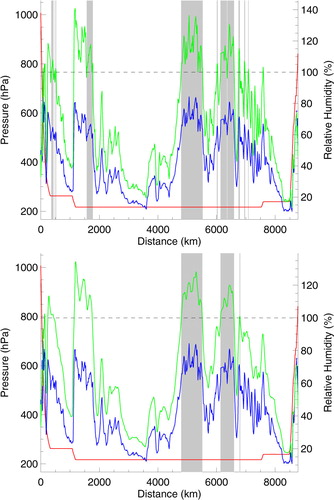
For investigations of large-scale features of ISSRs, we have to use a coarser resolution. Humidity data on a resolution of order O(10 km) includes mesoscale features (e.g. shallow cirrus convection, see Spichtinger, 2014). In fact, due to the high resolution a large-scale ISSR (with an extension to order O(10 km) or larger) could be separated into smaller pieces. However, such a separation would not be meaningful, since we are interested in the interaction with large-scale motions. Therefore, we use a running mean over N grid points for the original “high-resolution” data; i.e. we derive for each relative humidity value RHi _k at grid point k a mean value as given by5

The number of grid points N determines the new coarse resolution. For a resolution of order O(100 km), we choose N=7. The result of our ISSR detection method and the effect of averaging on the evaluated data can be seen in Fig. 1.

Grey shades indicate detected ISSRs, pressure is indicated by the red line and relative humidity values are represented by blue (RH) and green (RHi) lines, respectively. In the first part of the flight track, the impact of criterion (3) can be seen clearly. Due to a change in altitude/pressure the first ISSR at x~1000 km is not counted; this assures that if the aircraft is diving into an ISSR, which would lead to a shorter horizontal extension, this event is not recorded. Comparing the top and bottom panel, the effect of averaging is obvious, especially in the horizontal range 6000 ≤ x≤7000 km. Many small ISSRs either disappear or merge with the large-scale feature.

2.3. Separation into different classes

For detection of regional differences, the data are separated between extratropics (latitude >30 ° N or latitude <30 ° S) and tropics (30 ° S ≤ latitude ≤30 ° N). An ISSR is only counted to a regional category, if more than half of ISSR grid points belong to one region. Most MOZAIC flights are situated in the Northern hemisphere in the North Atlantic region.

Since troposphere and stratosphere have very different properties (e.g. in terms of water vapour mixing ratios, trace gases, temperature), it makes sense to separate between these regions for our investigations. Since in the MOZAIC project ozone is also routinely measured, this tracer can be used as indicator for tropospheric or stratospheric air. Chemical and thermal tropopause coincide often in altitude, thus this procedure is quite meaningful and was already used in former studies using MOZAIC data (e.g. Gierens et al., 1999). However, the determination of the tropopause using ozone only is not very accurate. Mixing of tropospheric and stratospheric air masses might lead to intermediate values, representing the relative influence of stratospheric air mixed into tropospheric air masses. As seen in the study by Cirisan et al. (2013) the ozone mixing ratio can be used as a measure for the influence of stratospheric air mixed into the considered air parcel. Ozone at the chemical tropopause also shows a seasonal cycle in the interval of mixing ratio 70 ≤ (Zahn and Brennikmeijer, 2003). Thus, we define the following vertical layers.

• Troposphere for mixing ratios

• Stratosphere for mixing ratios

• Layer between troposphere and stratosphere (tropopause region, or “in between”) for mixing ratios

An ISSR (or also a distance between ISSRs) is assigned to a vertical region (troposphere/in between/stratosphere), if the arithmetic mean over all measurements of ozone mixing ratio inside the ISSR met the criteria of the list indicated above.

Finally, we also distribute the detected ISSRs into six fixed pressure levels in the range 190 ≤ p≤340 hPa, as represented in Table 1.

Table 1. Definition of pressure levels for vertical distribution of ISSRs and distances between them

Number	1	2	3	4	5	6
p (hPa)	340–290	290–270	270–250	250–230	230–210	210–190

3. Results

In the time interval 1995–1999, a total number of 40 951 ISSRs could be identified in the original data. For the coarse resolution data (Δx~O(100 km)), a total number of 16 767 ISSRs were identified. Generally, we mostly concentrate on the evaluation of coarse data, since we are interested in the large-scale aspects of ISSRs.

3.1. Pathlengths

An ISSR is a three-dimensional object, which forms, develops and decays with time. Since we have to work with single aircraft flights on one-dimensional paths, we have to estimate the horizontal extension of an ISSR on a fixed flight level. For this purpose, we use pathlengths of ISSRs, i.e. the one-dimensional path of the aircraft through an ISSR. Flight routes are usually not strongly affected by weather pattern. Sometimes pilots try to shun storms, especially deep convection; however, for flights in the extratropics aircrafts can usually fly high enough to avoid such storms. For flights in the tropics, deep convection reaches into very high altitudes, thus the aircrafts have to fly around fully developed storms. Thus, there is probably no bias due to (avoided) weather patterns in the flight tracks and statistics of ISSR properties can be derived.

In a first step, the whole data set is evaluated without separation into horizontal or vertical regions. In Fig. 2, the probability density function (pdf) of pathlength for the two different resolutions (original: Δx~14 km, coarse: Δx~100 km) is shown.

Fig. 2 Pdfs of pathlengths of ISSRs as obtained from data with different resolution (blue: original resolution, red: coarse resolution). (a) Linear binning; (b) logarithmic binning.

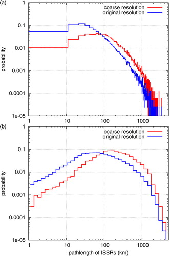
Both pdfs are skew with a long tail towards large values, similarly to the results by Gierens and Spichtinger (2000). In Fig. 2, top panel (a), the pdfs are shown for a linear binning. Due to the high skewness and a variation of pathlengths over some orders of magnitude, a representation in logarithmic binning (Fig. 2, bottom panel (b)) is more appropriate. The averaging leads either to a merging of smaller ISSRs to larger ones or to vanishing of single small ISSRs, respectively, leading to a shift in the pdfs. This behaviour is also represented in a shift in mean values and standard deviations σ _L (original: ; coarse: ). For the skew pdfs, the median of pathlengths med(L) is a more robust measure for the typical size of ISSRs, leading to the following values: med(L) _original =52 km, med(L) _coarse =142 km. Essentially, the maximum values in the logarithmic representation of the pdfs correspond quite well to these values (Fig. 2, panel (b)). In the following analysis, we will exclusively investigate pdfs in logarithmic binnings.

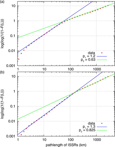
Gierens and Spichtinger (2000) found that the pdf of pathlengths for ISSRs might be represented by a Weibull distribution with a probability density f(L)=γL^{p −1} . For deriving fit parameters for the Weibull distribution, we use a so-called Weibull plot. We use the cumulative distribution of the data F(L) and plot log(L) against log(log(1/(1 − F(L)))). In case of a Weibull distribution (i.e. ), a straight line with slope p would appear in this representation. Using a linear fit we can derive the parameter p from the Weibull plot. This procedure was already used in former studies (Gierens and Brinkop, 2002; Spichtinger et al., 2003a). We find that for total data a combination of two Weibull distributions can be used for representing the pdfs for original and coarse resolutions; for each interval I ₁=(0,L _c ) and I ₂=(L _c ,∞) we find different parameters for original resolution (p ₁=1.2, p ₂=0.63) and coarse resolution (p ₁=1.3, p ₂=0.825), respectively. The value L _c indicate the transition in the regimes and corresponds quite well to the median values (original: L _c ~55 km, coarse: L _c ~150 km). The fits are shown in Fig. 3. Note that for original resolution the fit parameter p ₂=0.63 is close to the result p≈0.55 by Gierens and Spichtinger (2000).

Fig. 3 Weibull plot of pathlengths of ISSRs as obtained from data with different resolution and additional fits. (a) Original resolution; (b) coarse resolution.

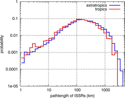
In a next step, we discriminate the whole data set by geographic regions, i.e. into extratropics and tropics, respectively. Since most MOZAIC aircrafts fly over the North Atlantic, the total number of ISSRs as found in the extratropics is about three times larger than the total number in the tropics. This feature is robust for both resolutions, original and coarse resolution. The pdfs of pathlengths for extratropical and tropical ISSRs are shown in Fig. 4 for the coarse resolution only. In fact, in extratropics the pathlengths of ISSRs are generally larger, whereas in the tropics generally smaller ISSRs could be found. This difference is also represented in mean pathlengths, standard deviation and median values (extratropics: , med(L) = 149 km; tropics: , med(L)= 124 km).

Fig. 4 Pdfs of pathlengths of ISSRs for different regions (blue: extratropics, red: tropics).

From former investigations we know that there is a seasonal variation in the occurrence of ISSRs (Spichtinger et al., 2003a, b). We investigate total data and data separated into extratropical and tropical measurements for different seasons, i.e. spring, summer, autumn and winter data (indicated by MAM, JJA, SON, DJF). Since the pdfs are very similar, differences might be seen better in cumulative distributions, as shown in Fig. 5 for extratropical data. Generally, the pdfs have the same shape as for the total data, as shown in Fig. 2.

Fig. 5 Cumulative distributions of pathlengths of ISSRs for different seasons as obtained for extratropical data in coarse resolution.

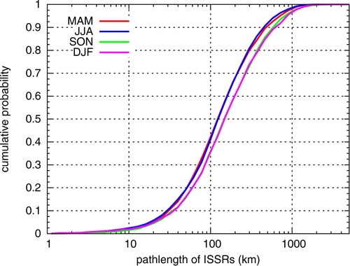
The mean values and standard deviations are represented in Table 2; Fig. 6 shows variations of median values.

Fig. 6 Median values of pathlengths for different regions, seasons and resolutions. The values can be found in Table 2.

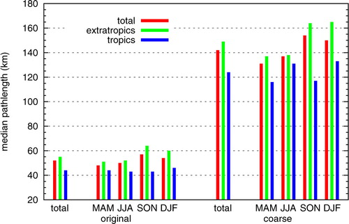
Table 2. Numbers, mean values, standard deviations and median values of pathlengths for different regions and seasons

Season	Resolution	N		σ L	med(L)
Total data
Total	Coarse	16 767	235	270	142
MAM	Coarse	3455	219	258	131
JJA	Coarse	5725	214	233	137
SON	Coarse	4575	258	297	154
DJF	Coarse	3012	256	300	150
Extratropical data
Total	Coarse	12 503	247	282	149
MAM	Coarse	2381	229	263	137
JJA	Coarse	4742	218	240	138
SON	Coarse	3580	277	317	164
DJF	Coarse	1800	284	324	165
Tropical data
Total	Coarse	4264	199	226	124
MAM	Coarse	1074	199	246	116
JJA	Coarse	983	192	194	131
SON	Coarse	995	188	197	117
DJF	Coarse	1212	215	253	133

There is seasonal variation in the extratropics. From cumulative distributions (Fig. 5) we see that pdfs for spring and summer are quite similar; the same is true for pdfs for autumn and winter, respectively. This feature can also be seen in the median values. In MAM/JJA smaller ISSRs occur (med(L)~138 km), whereas in SON/DJF larger values of pathlengths can be measured (med(L)~165 km). In addition, there is seasonal variation in numbers of ISSRs; most ISSRs occur in summer, whereas the minimum number is reached in winter. For tropical data, a different picture can be seen. The number of ISSRs is almost uniformly distributed over the course of the year. Pdfs for spring and autumn are quite similar and the same is true for pdfs for winter and summer. The difference between the pdfs is smaller than for the extratropical data; thus, the cumulative distributions are not shown. ISSRs in tropics are usually smaller in MAM/SON (med(L)~116 km) than in JJA/DJF (med(L)~131 km). In the total data, the variations are still noticeable; however, the variations in extratropics dominate the whole data.

From former studies we know that ice supersaturation in the stratosphere is quite seldom, although its occurrence is not completely improbable (Gierens et al., 1999; Spichtinger et al., 2003a). Therefore, we also investigate pathlengths of ISSRs for different dynamic regions. As indicated in Section 2.3, we distinguish between pure tropospheric air ( ppb), pure stratospheric air ( ppb) and air without clear tropospheric or stratospheric signature (“in between” or tropopause region, ppb). Since the pdfs are very similar in shape, in Fig. 7 the cumulative distributions of pathlengths in the different vertical regions are shown. The pdfs have generally the same shape as pdfs for total data.

Fig. 7 Cumulative distributions of pathlengths of ISSRs for different dynamic regimes, i.e. total data separated into troposphere/in between/stratosphere.

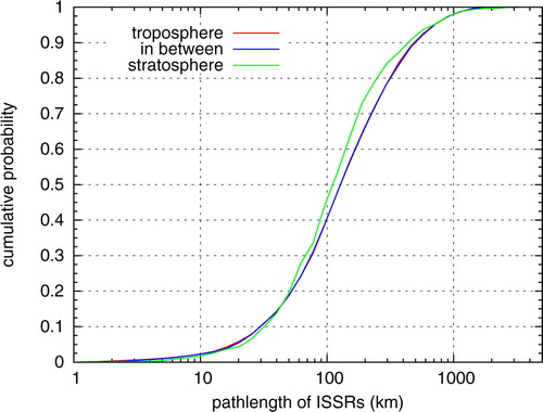
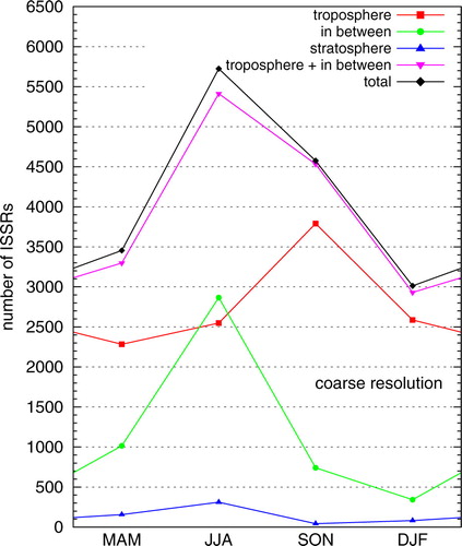
Most ISSRs are found in the troposphere (68.3% of all detected ISSRs), in the tropopause region still a reasonable amount of ISSRs could be identified (28.1%), while in the stratosphere just a marginal amount is detected (3.6%). The seasonal cycle of detected numbers of ISSRs is shown in Fig. 8. The total number shows a clear seasonal variability with a maximum for summer and a minimum during winter. The statistics is of course dominated by ISSRs in the troposphere and the tropopause region (“in between”). However, the numbers for the separate layers show an interesting behaviour. In the tropopause region, the seasonal cycle is the same as described for the total data. However, for pure tropospheric ISSRs the whole cycle and thus the maximum is shifted by one season (i.e. 3 months).

Fig. 8 Seasonal cycle of number of ISSRs as obtained for different dynamic regimes.

The typical sizes of ISSRs (median values) are the same for tropospheric ISSRs and for ISSRs occurring close to the tropopause (med(L) = 143 km), whereas ISSRs in the stratosphere are much smaller (med(L) = 124 km). There is also a seasonal cycle in pathlengths of ISSRs in different dynamic regions. Pdfs for pathlengths of ISSRs for spring and summer are quite similar (med(L)~130 km), the same is true for pdfs for autumn and winter (med(L)~154 km). Near the tropopause, pdfs for spring, summer and winter agree (med(L)~140 km), the pdf for autumn, however, leads to larger pathlengths of ISSRs (med(L) = 157 km). For stratospheric ISSRs, the statistics are not good enough (small number of events) to derive a reasonable seasonal cycle. The values are represented in Fig. 9 and are repeated in Table 4.

Finally, we can observe that for a fixed pressure level distribution there is strong variation in number and pathlengths of ISSRs. The number of ISSRs increases with height (i.e. decreasing pressure) over the first three levels. At levels 3 and 4 (270 ≤ p≤230 hPa) most ISSRs can be found; then, the number of ISSRs is decreasing again. For the pathlengths, we observe a different behaviour. The mean pathlength is increasing with decreasing pressure; the maximum in the median pathlengths can be found at pressure level 5 (250 ≤ p≤230 hPa). The values for coarse resolution and original data are reported in Table 4.

Table 3. Numbers, mean values, standard deviations and median values of pathlengths for different atmospheric levels (troposphere/in between/stratosphere)

Season	Resolution	N		σ L	med(L)
Troposphere
Total	Coarse	11 209	235	267	143
MAM	Coarse	2283	216	253	130
JJA	Coarse	2548	202	211	134
SON	Coarse	3791	254	286	154
DJF	Coarse	2587	257	297	151
In between
Total	Coarse	4965	236	273	143
MAM	Coarse	1015	229	262	138
JJA	Coarse	2866	226	249	142
SON	Coarse	741	283	352	157
DJF	Coarse	343	242	291	137
Stratosphere
Total	Coarse	593	213	287	124
MAM	Coarse	157	201	303	120
JJA	Coarse	311	200	239	123
SON	Coarse	43	184	215	131
DJF	Coarse	82	302	411	155

Table 4. Numbers, mean values, standard deviations and median values of pathlengths for different vertical pressure levels in both resolutions

Level (hPa)	Resolution	N		σ L	med(L)
1 (340–290)	Original	1492	81	107	44
2 (290–270)	Original	3728	97	145	48
3 (270–250)	Original	11 448	109	164	54
4 (250–230)	Original	11 591	114	186	52
5 (230–210)	Original	9788	129	212	55
6 (210–190)	Original	2521	112	177	52
1 (340–290)	Coarse	547	164	174	115
2 (290–270)	Coarse	1476	199	218	127
3 (270–250)	Coarse	4676	225	248	141
4 (250–230)	Coarse	4778	241	284	143
5 (230–210)	Coarse	4163	264	302	155
6 (210–190)	Coarse	1039	230	258	139

3.2. Distances between ISSRs

Although in former investigations, horizontal extensions of ISSRs were investigated (Gierens and Spichtinger, 2000; Diao et al., 2014), the distance between ISSRs was never investigated before. Actually, there are only few studies for other clouds available. We are only aware of the study by Joseph and Cahalan (1990). We define the distance between ISSRs as the distance between two nearest neighbour ISSRs along the flight track and at the same pressure level. The pressure level restriction leads to a small reduction in the identified number of ISSRs for the evaluation of intercepts. We separate between distances of ISSRs in different geographic regions (total/extratropics/tropics) as well as in dynamic regions (troposphere/in between/stratosphere).

In Fig. 10, the impact of the change in resolution (original vs. coarse) on the distribution of distances is shown. As for pathlengths of ISSRs the distances generally become larger for the coarse resolution data. As indicated in Fig. 1 small ISSRs disappear or merge with larger ones. Thus, the distances between ISSRs should also be larger for coarse data.

Fig. 9 Median values of pathlengths in different dynamic regions, total and seasonal. The values can be found in Table 3.

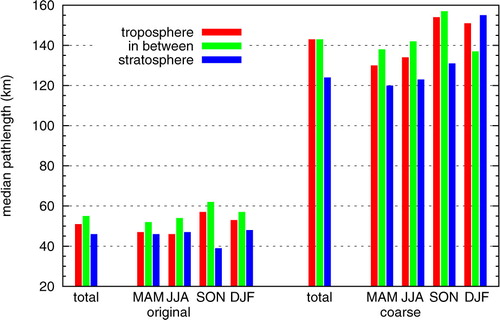
Fig. 10 Pdfs of distances between ISSRs as obtained from data with different resolution (blue: original resolution, red: coarse resolution). (a) Linear binning; (b) logarithmic binning.

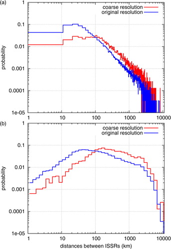
The shift is obvious in mean values , standard deviations σ _D and, more robust, in median values med(D). For the original resolution, we obtain a median of med(D) = 66 km, whereas for coarse data resolution the value is shifted to med(D) = 217 km.

In contrast to the pathlength distributions, the pdfs of distances are less steep (in the double logarithmic scale). For the different geographic regions, i.e. distances of ISSRs in the extratropics and tropics, respectively, there is almost no difference in the pdfs (not shown).

For the split into seasons, a weak seasonal cycle can be found for extratropical and tropical data, respectively. For the extratropics, we found a seasonal cycle in the total number of distances between ISSRs, similarly to the cycle in pathlengths of ISSRs; in summer a maximum value could be found whereas the minimum occurs during winter. The typical size of a distance shows a weak maximum in summer and minimum values in winter and spring. For the tropics, the number of events is almost uniformly distributed over the seasons. As for the pathlengths of ISSRs, maximum values for distances can be found in spring and autumn, respectively. However, the signal is much weaker than for pathlengths of ISSRs. Finally, we can state that the pdfs are very similar, even in cumulative distributions almost no variation can be seen. Mean values, standard deviations and median values of distances between ISSRs for total, extratropical and tropical data are reported in Table 5.

Table 5. Numbers, mean values, standard deviations and median values of distances between ISSRs for different regions and seasons

Season	Resolution	N		σ D	med(D)
Total data
Total	Coarse	7741	514	753	217
MAM	Coarse	1527	504	754	218
JJA	Coarse	2750	525	754	218
SON	Coarse	2128	514	772	217
DJF	Coarse	1336	503	715	215
Extratropical data
Total	Coarse	5427	506	742	211
MAM	Coarse	957	474	723	200
JJA	Coarse	2223	536	763	218
SON	Coarse	1580	495	741	212
DJF	Coarse	667	478	692	199
Tropical data
Total	Coarse	2314	534	777	234
MAM	Coarse	570	554	801	251
JJA	Coarse	527	479	712	218
SON	Coarse	548	572	854	240
DJF	Coarse	669	528	736	229

Now we separate the distances between ISSRs into levels of different dynamic characteristics as before (troposphere/in between/stratosphere). The pdfs are shown in Fig. 11, mean values, standard deviations and median values are reported in Table 6. There is a remarkable difference in the pdfs for tropospheric data (including also data close to the tropopause, i.e. “in between”) and stratospheric data. As a general feature the median values of distances between ISSRs increase with levels (from low to high altitudes). In the dry stratosphere, the largest distances can be found. While the pdfs for both lower levels are still similar in shape, the pdf of stratospheric data looks very different, it is clearly shifted to high values, whereas the amount of small distances is strongly reduced compared to the other pdfs. At large values of D there is a strong scattering in stratospheric data (not shown); this is also due to the low number of events. For both lower levels, a seasonal cycle can be seen, similarly to the cycle in the pathlengths of ISSRs for tropospheric data and data close to the tropopause. However, the cycle is less pronounced than in cases of pathlengths of ISSRs.

Fig. 11 Pdfs of distances between ISSRs for different dynamic regimes, i.e. total data separated into troposphere/in between/stratosphere.

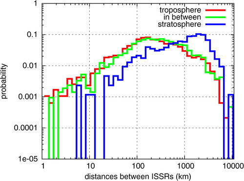
Table 6. Numbers, mean values, standard deviations and median values of distances between ISSRs for different atmospheric levels (troposphere/in between/stratosphere)

Season	Resolution	N		σ D	med(D)
Troposphere
Total	Coarse	4758	407	623	179
MAM	Coarse	965	419	616	182
JJA	Coarse	1091	367	601	164
SON	Coarse	1578	406	635	177
DJF	Coarse	1124	435	631	194
In between
Total	Coarse	2125	462	691	224
MAM	Coarse	411	468	756	227
JJA	Coarse	1168	400	612	193
SON	Coarse	400	571	746	326
DJF	Coarse	146	647	852	293
Stratosphere
Total	Coarse	858	1240	1085	1014
MAM	Coarse	151	1150	1139	794
JJA	Coarse	491	1173	990	952
SON	Coarse	150	1504	1273	1256
DJF	Coarse	66	1344	1069	1147

3.3. Relative humidity at ISSR boundaries

We have investigated running mean data as obtained from data at resolution of Δx~14 km in order to investigate large-scale features. However, the question arises how clear we can distinct between different large-scale ISSRs, i.e. how sharp are the boundaries between different features. From former investigations using ECMWF data we know that the horizontal gradients of RHi might be very sharp for special dynamic features (e.g. ISSRs driven by warm conveyor belts or waves, see Spichtinger et al., 2005a, b). For in situ data, this issue has not been investigated before on a statistical basis. For this purpose, we again evaluate the edges of ISSRs as represented in the “original resolution”, i.e. for Δx~14 km. For determining the separation of ISSRs in terms of RHi, we investigate the distance from the last measurement inside the ISSR (i.e. RHi>100%) to the measurement point where relative humidity falls below a certain threshold (RHi<RHi _t ) for the first time. We use four different values for RHi _t =95/90/80/70%. For these fixed values, we obtain pdfs for the distance.

High values of RHi _t (e.g. RHi _t ~95%RHi) represent a weak separation of ISSRs from their subsaturated environment. Neighbouring ISSRs separated by weakly subsaturated values might even belong to the same large-scale feature. Low values of RHi _t (e.g. RHi _t ~70%RHi) probably indicate a clear separation of ISSRs by subsaturated air masses. Neighbouring ISSRs might not belong to each other in a dynamical sense.

In Fig. 12, pathlengths of RHi are shown, i.e. the distance from a boundary of an ISSR in subsaturated air until the threshold is reach for the first time. Again, we show linear binning (top panel (a)) and a logarithmic binning (bottom panel (b)) for representing the shape of the distributions in a meaningful way. The pdf for RHi _t =95% shows that in most cases the typical distance is very small, mostly in the order O(10 km), and they rarely exceed values on order O(100 km). Thus, ISSRs are often surrounded by a halo of slightly subsaturated air on order of few tens of kilometres. The halo belongs to the ISSR in a large-scale sense. The running mean is smearing out this feature and ISSRs, which are close to each other connected by the slightly subsaturated halo are merged. By comparing the distributions of distances between ISSRs in the original resolution (Fig. 10) and the pdf of pathlengths of RHi at high RHi _t ~90/95%, we note that values in the order of O(10 km) occur quite frequently in both pdfs. This is also an indication for the described phenomenon; weakly separated ISSRs might belong to the same large-scale feature.

Fig. 12 Pathlengths of relative humidity as obtained from the original data for different thresholds RHi _t =95/90/80/70 %. (a) Linear binning of the data; (b) logarithmic binning.

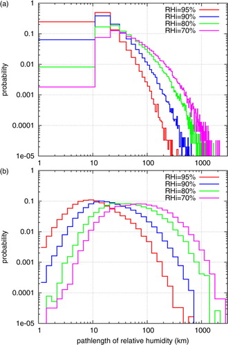
There is a clear shift in the pdfs of pathlengths of RHi towards larger pathlengths, when the threshold RHi _t is changed to smaller values (Fig. 12, panel (b)). A sharp boundary with a decrease in RHi to low values (i.e. RHi _t =70%) within a short distance is less frequently observed. Although (large-scale) ISSRs are clearly separated from the subsaturated air, the distance to a decrease in RHi to low values is usually larger (on order O(100 km)).

Mean values, standard deviations and median values for distances until RHi=RHi _t is reached are given in Table 7. The number of pathlengths of RHi is decreasing with decreasing threshold. This can be interpreted as follows. Most ISSRs are located in a slightly subsaturated air, the next ISSR can be reached along the flight track without reaching low values of RHi. In contrast, clear separation of ISSRs by subsaturated air occurs only if the ISSRs belong to spatially different large-scale features. Generally, the number of ISSRs driven by large-scale motions is smaller than ISSRs on cloud scale, as found in the original resolution data.

Table 7. Numbers, mean values and standard deviations for pathlengths of RHi until the threshold RHi _t is reached. Here, all data in original resolution are used without separation into horizontal or vertical regions

Season	RHi t	N			med(L RHi )
Total	95	60 631	14	16	9
MAM	95	12 963	15	18	9
JJA	95	21 702	12	14	8
SON	95	15 598	14	17	9
DJF	95	10 368	15	18	9
Total	90	50 189	29	35	17
MAM	90	10 645	31	38	18
JJA	90	18 050	26	31	16
SON	90	12 985	29	35	17
DJF	90	8509	31	39	18
Total	80	38 409	63	80	37
MAM	80	8153	68	87	39
JJA	80	13 909	57	70	34
SON	80	9882	64	78	38
DJF	80	6465	70	90	40
Total	70	31 404	104	126	62
MAM	70	6756	112	139	65
JJA	70	11 364	93	113	55
SON	70	8027	106	124	65
DJF	70	5257	115	138	69

If the horizontal separations (with respect to RHi) are distributed into seasons, again a cycle can be seen. For summer, the pathlengths of RHi are usually smaller; thus, ISSRs are more clearly separated from subsaturated air in the environment. For winter, the pathlengths of RHi are somewhat larger and the transition to subsaturated air is smoother.

We also investigate pathlengths of RHi on different pressure levels. Of course, the seasonal cycle in ISSR numbers can also be seen for pathlengths of RHi. In addition, we find that with increasing altitude (decreasing pressure) the mean pathlengths of RHi slightly increase. Thus, at high levels, the boundaries between ISSRs and the surrounding subsaturated air are less sharp and gradients are weaker. This feature can be seen most prominent for the lowest threshold RHi _t =70%. In this case, the mean value is increasing from to . The median values changes from med(L _RHi ) = 34 km to med(L _RHi ) = 84 km. The exact values for the numbers, mean values and standard deviations as well as median values are represented in Table 8.

Table 8. Numbers, mean values and standard deviations for pathlengths of RHi until the threshold RHi _t is reached. All data in original resolution here are used with separation into different pressure levels

Level (hPa)	RHi t	N			med(L RHi )
1 (340–290)	95	2292	9	11	6
2 (290–270)	95	5637	11	13	7
3 (270–250)	95	17 354	13	15	8
4 (250–230)	95	16 966	14	17	9
5 (230–210)	95	14 220	16	18	10
6 (210–190)	95	3659	16	18	10
1 (340–290)	90	1933	19	24	12
2 (290–270)	90	4739	21	26	13
3 (270–250)	90	14 372	26	30	16
4 (250–230)	90	14 032	30	37	18
5 (230–210)	90	11 664	33	41	20
6 (210–190)	90	3057	36	40	21
1 (340–290)	80	1487	37	45	22
2 (290–270)	80	3665	45	55	27
3 (270–250)	80	10 937	56	67	34
4 (250–230)	80	10 676	68	84	40
5 (230–210)	80	8980	75	93	44
6 (210–190)	80	2404	82	94	49
1 (340–290)	70	1256	59	75	34
2 (290–270)	70	2980	72	88	43
3 (270–250)	70	8918	92	105	57
4 (250–230)	70	8720	111	132	67
5 (230–210)	70	7363	124	149	73
6 (210–190)	70	1963	133	149	84

Further investigation of pathlengths of RHi is difficult. In fact, mean gradients of RHi, i.e. (100% − RHi _t )/med(L), do not vary significantly and their variations are hard to interpret. Thus, we leave this topic for future work in case studies.

4. Discussion

There are remarkable differences in pdfs of ISSRs and distances between ISSRs for different geographic regions, i.e. extratropics vs. tropics and different atmospheric levels (dynamic separation and pressure levels, respectively).

In the tropics, there is a weak seasonal cycle visible in the pdfs. Upward motions are induced in the environment of (deep) convection; these vertical motions are probably the main driver for the formation of ISSRs. It is clear that these updrafts must be moderate, otherwise the whole system would be dominated by convective clouds. Convection is active in the tropics without a strong seasonal cycle. The main convective regions follow the intertropical convergence zone (ITCZ); however, even (far) away from the ITCZ convection activity can be observed. In addition, the tropical tropopause is usually located well above standard aircraft flight levels; thus, MOZAIC aircrafts will almost exclusively fly in tropospheric air in the tropics. The main environmental conditions as temperature profiles and vertical upward motions do not change qualitatively with seasons in the tropics. It is reasonable also that pathlengths (and distances) of ISSRs do not show a strong seasonal cycle.

For the extratropics, the situation is much more complicated. There are two (connected) large-scale features, which change over the course of the year and thus influence properties of ISSRs.

First, storm activity (especially over the North Atlantic) is strongly influenced by seasons. Low pressure systems and their associated frontal systems are most active (and vigorous) during autumn/winter time. During summer, storm activity is strongly reduced over Northern Atlantic and the weather situation is often dominated by stationary high-pressure systems.

The second feature is actually crucially connected with synoptic weather scales and storms; however, it is currently easier to present these features separately. In the extratropics, the tropopause has a strong seasonal cycle in altitude, crucially depending on low and high-pressure systems (e.g. Seidel and Randel, 2006; Grise et al., 2010; Kunz et al., 2011). In hemispheric winter, the tropopause is located at very low altitudes, whereas in summer (i.e. at high-pressure systems) the tropopause reaches quite high altitudes (e.g. Birner, 2006; Gettelman et al., 2011). Thus, in the extratropics the tropopause is always located in the possible altitude range of commercial aircrafts.

These two features are responsible for the change in frequency of occurrence of ISSRs as well as for the change in pathlengths. In autumn and winter, the enhanced storm activity leads to largely extended frontal systems, thus the pathlengths should get larger; the vertical upward motions are located at the extended fronts of the system. On the other hand, in winter the tropopause is located at low altitudes. Commercial aircrafts always fly similar routes without seasonal changes. Thus, the aircrafts fly in the dry stratosphere for a longer time and therefore less ISSRs can be found. During summer, the tropopause is usually located at high altitudes; thus aircrafts fly more often in the troposphere and the tropopause region, than in winter time. Therefore more ISSRs can be detected; this leads to the seasonal cycle in number of ISSRs. Generally, it is not really clear why in summer the pathlengths are smaller. Then ISSRs develop mostly in high-pressure systems; thus, the internal structure of these systems might influence the pathlengths. However, this issue cannot be solved without a very detailed inspection of ISSRs in high-pressure systems on a case by case basis, which is beyond our statistical investigation.

The increase of pathlengths with height (i.e. with decreasing pressure) is also not really understood. One explanation might be that climbing in the troposphere from below towards the tropopause (an “inversion layer”) vertical velocities are more damped. This damping might also smear out variations in updrafts and leads to a more homogeneous updraft region (with lower values of vertical velocity due to damping). This large and more homogeneous region might then lead to larger regions of ice supersaturation. But not only updrafts but also downdrafts – which introduce subsaturation – might be weaker due to the damping. Thus, larger ISSRs could exist in higher levels due to (a) more homogeneous updraft regions and/or (b) a slower removal of ice supersaturation by slower downdrafts.

For distances between ISSRs, some features as for the pathlengths can be seen. The number of ISSRs determines the number of distances, thus a seasonal cycle similar to the cycle of pathlengths is obvious. For the extension of distances between ISSRs, it is not clear which mechanism is dominant, leading to the distribution of distances. For extratropical summer, the mean distance is much larger than for distances in winter time. Since in summer more but smaller ISSRs can be found, maybe the distribution of ISSRs relative to each other is affected in the following sense. More “horizontal extension” (i.e. space in the troposphere/tropopause region at one pressure level) is available for the spatial distribution of ISSRs. In fact, it seems that agglomeration of ISSRs on small range is seldom; ISSRs tend to prefer long distances between nearest neighbours. The reason for this feature is unclear; probably, it depends on large-scale dynamic features.

Investigations on RHi at edges of ISSRs give some additional information about the structure. ISSRs are usually surrounded by slightly subsaturated air. The mean distance until a threshold of high RHi values (e.g. RHi _t =95/90%) is quite small, thus this halo has a short extension (on order O(10 km)). The running mean procedure in order to derive large-scale features is usually smeared out, i.e. the halo is counted as supersaturated air, which is meaningful in terms of our investigations. Lower thresholds of RHi _t are reached less frequently, the distance to low thresholds is larger.

The seasonal variation can be seen, however, to be quite small. The shorter mean distances during summer can perhaps be explained by the general smaller pathlengths of ISSRs; thus, also the halo is smaller. The variation in height is more pronounced. The halo gets larger with decreasing pressure. Also this feature might be explained by the damping characteristics of the tropopause region (and the stratosphere, too), as indicated above. Less various vertical updrafts lead to a more homogeneous region of vertical updrafts; thus, the boundaries between ISSRs also get less pronounced.

5. Origin of ice supersaturation

As indicated in the introduction, the origin of ice supersaturation in the upper troposphere and lowermost stratosphere is not clear. By inspecting the definition of relative humidity over ice and the resulting total derivative, it is clear that changes in temperature, pressure and specific humidity (i.e. water vapour mixing ratio) can change relative humidity. Probably the main processes for changing cloud-free relative humidity in the tropopause region are (a) adiabatic processes and (b) mixing processes.

In recent studies, high-resolution measurements show large variability of RHi on a small scale (order of O(1 km) or even smaller) along horizontal flight tracks (Diao et al., 2014). Variability of RHi were strongly connected to variations in water vapour mixing ratios, whereas the temperature did not change significantly along the flight track. Thus, it was conjectured that the driver for ice supersaturation is not a temperature change (as in adiabatic processes) but merely a change in specific humidity. This would point more in the direction of mixing or other (diabatic) processes.

We present here a distinct interpretation of (high-resolution) variations in relative humidity. We propose the idea that most of RHi variations result from pure adiabatic processes (cooling by expansion) and the accompanying variations in specific humidity are simply resulting from the transport of water vapour. For explaining our conjecture in details, we carry out very simple simulations that include the main processes.

5.1. Model description

In order to investigate small-scale variations and their relationship to large-scale features as well as changes in relative humidity, we include important aspects in a very simple model. We assume pure large-scale vertical motion for air parcels measured at a constant horizontal flight track. In our case, we set the flight altitude to a fixed value z ₀=10000 m. Each air parcel ascended from a certain altitude with a constant but variable vertical velocity during a constant time t=4 hours. The vertical velocity is changed randomly (see below for details), thus each air parcel k started at a different altitude z _k,start =z ₀−w·t. We also prescribe a temperature profile with a constant Brunt–Vaisala frequency N=0.005 s⁻¹, as typical for the upper troposphere, with a surface temperature of T _s =288 K. This resulted into a temperature of T=206.71 K at flight level z ₀. In addition, an exponential pressure profile is prescribed with a scale height h=8 km. The start temperature of the parcel T _k,start at height z _k,start can be determined from the temperature profile. Since we assume a pure adiabatic process, the temperature of the lifted air parcel at z ₀ can be calculated. For example, a constant vertical velocity of w=0.05 m s⁻¹ would result into a start height z _start =9280 m, a start temperature T _start =211.7 K and a temperature T=206.33 K at z ₀. We assume that the relative humidity over ice at the starting points has the same fixed value changed by a random spread. The fixed value is set to , the change is uniformly distributed with a width of ±5% (i.e. 48 ≤ RHi _start ≤58%). For the constant value of w ₀=0.05 m s⁻¹, an ascent with the constant mean value would result into a relative humidity value of RHi=103.14% at flight level. With this setup, we want to assure that we frequently observe supersaturated conditions at flight level z ₀. We completely neglect changes in q due to cloud processes or mixing along the ascent, we are just interested in adiabatic processes.

It is reasonable to assume that in synoptic scale systems triggering large-scale upward motions the vertical velocity is not exactly the same everywhere but might differ in a certain range (it should be still of “synoptic” scale, i.e. w≤8 − 10 cm s⁻¹). In addition, variations on smaller scales (mesoscale, cloud scale and small-scale) might occur due to embedded features at smaller scales, e.g. turbulence, convective cells or gravity waves. For prescribing the vertical velocity in a “realistic” way, we want to mimic variations on different scales. For this purpose, we superimpose random variations on different scales but with the assumption that the large-scale component is dominating, variations at smaller scales should be smaller. During the simulation, the horizontal coordinate is computed with an increment of Δx=100 m, i.e. x _i =x _i−1+Δx. This resolution is similar to that of high-quality measurement techniques for measurements at research aircrafts (see, e.g., Zöger et al., 1999; Zondlo et al., 2010). The vertical velocity is composed by the following contributions:

• Large-scale of order O(100 km): each 100 km we choose a Gaussian distributed random velocity component Δw _L (σ _L =0.5 cm s⁻¹, mean value )

• Mesoscale of order O(10 km): each 10 km we choose a Gaussian distributed random velocity component Δw _M (σ _M =0.25 cm s⁻¹, mean value )

• Cloud scale of O(1 km): each 1 km we choose a Gaussian distributed random velocity component Δw _C (σ _C =0.1 cm s⁻¹, mean value )

• Small scale of O(100 m): At each grid point we choose a uniform distributed random velocity component Δw _S in the interval [−0.1, 0.1] cm s⁻¹, mean value .

Thus, we have at each grid point a vertical velocity as given by6

which includes all relevant scales with a dominant large-scale component. The simulation is carried out for n=2.10⁶ grid points.

Our assumption of a constant vertical velocity for a long time of 4 hours might be too idealised. However, one could assume changes in vertical velocity during the ascent. In principle, this would result into qualitatively similar simulations, i.e. air parcels measured at a certain horizontal flight path originate from (slightly) different vertical levels below. For showing the main phenomenon, we use this (maybe oversimplified) setup.

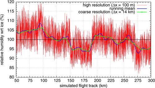
In a second step, we want to mimic the coarse resolution as measured by MOZAIC, i.e. on a horizontal scale of Δx~14 km. For this purpose, we calculate a running mean value for RHi from the high-resolution data, using Gaussian weights and a grid interval of N=141. In addition, we choose grid points with this coarse resolution from the running mean data. Figure 13 shows an example for these three data sets in the interval 50 ≤ x≤300 km.

Fig. 13 Example of relative humidity along a simulated flight track. Shown are high-resolution data (red), running mean (blue) and coarse resolution as obtained from running mean data (green) in the interval 50 ≤ x≤300 km.

5.2. Simulation results

In Fig. 14, a short part of the simulated flight track is shown for relevant variables RHi, T, q and w; the total range of variations in these variables is reported in Table 9. Our high-resolution simulation shows a huge variability of relative humidity in the range 68.6 ≤ RHi≤157.5. The relative humidity of a single grid point (air parcel view) has increased from the start value RHi _start at start level z _start by an adiabatic expansion during a large-scale updraft with a constant vertical velocity (in the range 2.60 ≤ w≤7.67 cm s⁻¹). The water vapour mixing ratio remains constant during the upward motion, since we neglect mixing and cloud processes, i.e. at flight level z ₀ we “measure” the same mixing ratio as at the start point z _k,start . Since the water vapour originated from different vertical levels with different temperatures, there is a large variability in q between different (subsequent) grid points. On the other hand, the variability in temperature in the different grid points is quite small, i.e. on order of O(0.1 k). At a first glance, this is surprising, since we know that the process changing RHi at the ascent is adiabatic change of temperature (and pressure). The solution of this discrepancy can be found in the temperature profiles, as shown in Fig. 15. Here, the adiabatic ascents from the lowest and the highest level (8896.5 m and 9624.4 m) in the simulation are shown, respectively. Since the angle between the temperature profile with its constant Brunt–Vaisala frequency (N _profile =0.005 s⁻¹) and the adiabatic pathways is very small and the distance of the ascent is quite short (Δz<1200 m), the temperature difference between the two air parcels after the ascent at flight level z=10000 m is really small (ΔT<0.4 K). If we would have started with a neutral profile, the temperature difference between the air parcels would have been zero. On the other hand, for profiles with larger Brunt–Vaisala frequency the variations would increase; however, for typical tropospheric values (N~0.01 s⁻¹) differences in temperature variations do not exceed values on order O(1 K).

Fig. 14 Variations of different variables (RHi, w, q and T) relevant for the small structure of ISSRs.

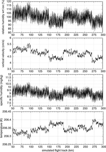
Fig. 15 Vertical temperature profile and adiabatic ascents for the lowest and highest levels occurring in the simulation.

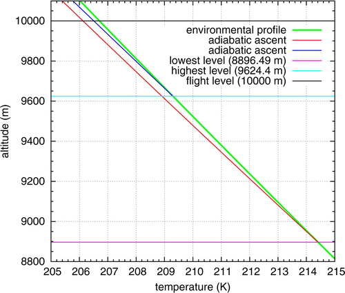
Table 9. Range of variables for start conditions (vertical velocity w and start level z _start ) and obtained at flight level z=10000 m (temperature T, relative humidity RHi and specific humidity q) during the simulation

w (cm s^−1)	Start level z (m)	T (K)	RHi (%)	q (mg/kg)
2.60 ≤ w≤7.67	8896.5 ≤ z start ≤9624.4	206.126 ≤ T≤206.509	68.6 ≤ RHi≤157.5	6.38 ≤ q≤13.88

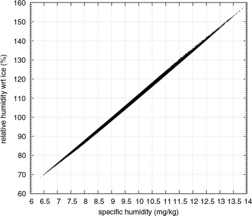
If we instead investigate variations of variables RHi, T and q at a horizontal flight level (see, e.g., Fig. 14), we could assume that relative humidity variations are mostly triggered by variations in q. However, in our simulation it is clear that relative humidity is exclusively increased by adiabatic temperature and pressure changes and the variation in q is just a transport phenomenon; neighbouring air parcels originate from different vertical levels with different start temperatures and humidities. This feature of variations at a horizontal flight level can be seen in any case of vertical ascents with only marginal or negligible mixing of air. Cloud processes would just damp humidity variations, since water vapour would be consumed or set free by growing or evaporating ice crystals. Thus, we have a reasonable theoretical explanation for high-resolution RHi variations, as originating (almost) solely from adiabatic ascents starting at (slightly) different vertical levels (i.e. pure transport effects). For investigating such high-resolution variations, it is important to use a Lagrangian point of view, i.e. following the air parcels for the investigations. An analysis just along the horizontal flight track (Eulerian point of view), as carried out by Diao et al. (2014) would lead to misleading conclusions, and in fact, we would not be able to explain the origin of large differences in specific humidity on a very small scale. As in the evaluations by Diao et al. (2014), a strong correlation of q and RHi data on the flight level can be detected in our simulation (c.f. Fig. 16). In contrast, the temperature variation (measurements at a distinct flight level) is quite small; however, the origin of high RHi is adiabatic ascent, thus temperature decreases and absolute humidity (i.e. water vapour mass) is just transported.

Fig. 16 Correlation between specific humidity and relative humidity for the high-resolution simulation data.

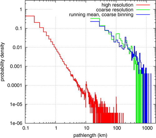
In the simulation, we have investigated high-resolution variations of RHi, which looks very similar to real data as found during research flights (e.g. Lee et al., 2004; Krämer et al., 2009; Diao et al., 2014). There is still the question, if and how MOZAIC data on low resolution as investigated in the prior sections is related to high-resolution variations. For investigating this issue, we evaluate the high-resolution simulation in terms of pathlengths. The simulation shows a huge variability, thus most ISSRs have pathlengths in the range of few 100 m. This is represented in the mean value of m, i.e. of a similar order than reported by Diao et al. (2014) for their high-resolution data with horizontal resolution of Δx~230 m. If we choose either a coarse resolution from the running mean or evaluate running mean data on a coarse grid corresponding to the MOZAIC resolution of Δx~14 km, we obtain similar pathlength distributions as for the MOZAIC data. The pathlengths statistics are shown in Fig. 17. This shows that high-resolution data and coarse resolution data in principle show the same phenomenon in terms of pathlengths of ISSRs. Coarse resolution data is not able to show the whole fine scale structure as high-resolution measurements on research flights. However, if we are interested in large-scale features of ISSRs, i.e. ISSRs driven by large-scale dynamics, then coarse resolution data (e.g. MOZAIC) is able to represent the important features. Additionally, it is clear that the finding by Diao et al. (2014) of much smaller pathlengths for high-resolution data is not in contradiction with the results as obtained from MOZAIC data in this study.

Fig. 17 Pdf of pathlengths of ISSRs as obtained from the high-resolution simulation data (red), running means on coarse binning (blue) and coarse resolution (green).

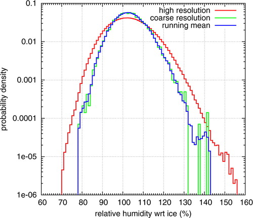
Finally, we investigate relative humidity statistics as obtained from the three data sets (high-resolution, running mean, coarse resolution). The result is shown in Fig. 18. The high variation in relative humidity and especially the high values of RHi are driven by the variations in temperature (originating from different starting levels). Similar findings were obtained in a former theoretical study (Kärcher and Haag, 2004). In fact, RHi data on all thee resolutions show the same qualitative behaviour, especially a quasi-exponential decay in probability for high supersaturations. In coarse resolution data (running mean and coarse grid), generally extreme values are more rare than for the high-resolution data. Although this is not a proof for MOZAIC data quality, the results point into the direction that even for coarse data the detection of high relative humidities might be possible.

Fig. 18 Pdfs of RHi as obtained from the high-resolution simulation data (red), running means on coarse binning (blue) and coarse resolution (green).

We conclude this section with few remarks:

• We have also carried out the simulation with a constant start value for relative humidity (RHi=53%). Actually, the results remain qualitatively the same. The random spread in the initial relative humidity value just lead to a smoothing in the distributions. For instance, for the high-resolution data the pathlength statistics would show more distinct peaks at the prescribed scales x=10/100 km and integer multiplies of them. The essence of the study remains the same. The large variation in relative humidity on a small scale is a pure transport phenomenon, lifting moist air from slightly different vertical levels to the flight level; the relative humidity is purely driven by temperature and pressure change along the lifting pathway although investigating data at a constant flight level it seems that variation in specific humidity would mainly cause the change in RHi.

• Our prescribed vertical velocities are just used to motivate large-scale patterns. In fact, each adiabatic ascent of air parcels would result into these small temperature variations. For example, shallow cirrus convection as described by Spichtinger (2014) results also into small temperature variations at a certain level, although the vertical velocities are much larger in this case. The determining factor is not the vertical velocity but the adiabatic process.

6. Conclusions

We have evaluated data from the MOZAIC project for the years 1995 to 1999 in order to determine properties of ISSRs in the UTLS region. We mostly concentrate on large-scale features of ice supersaturation. Therefore, we used a running mean procedure for filtering the data from small-scale variations; then, we evaluated the new data with a resolution of order O(100 km). We investigated horizontal properties of ISSRs as pathlengths (as a measure for horizontal extensions), distances between ISSRs and horizontal RHi gradients at the boundaries of ISSRs. We could derive the following results

1. Pathlengths of ISSRs have typical values (median) on order O(150 km); in tropics ISSRs are generally smaller than in the extratropics.

2. There is a strong seasonal cycle for extratropical ISSRs; most ISSRs are found during summer, and a minimum is found at wintertime. This statistics is probably biased by the fixed flight levels of commercial aircrafts in contrast to the seasonal cycle of the tropopause. In addition, there is also a seasonal cycle for the mean pathlengths with a maximum in autumn and winter and a minimum in summer. The reason for that remains unclear, although storm activity and associated frontal systems may influence pathlengths of ISSRs. There is also a weak seasonal cycle for tropical data of ISSR pathlengths.

3. For ISSRs in the troposphere and in the tropopause region, similar seasonal cycles could be found, although there is a shift in the seasonal cycle between these layers. Most ISSRs are found in troposphere/tropopause region, and ISSRs occur only marginally in the dry stratosphere.

4. Distances between ISSRs have typical values on order O(200 − 250 km). There is a seasonal cycle in number of distances, as given by the seasonal cycle of ISSRs. Also for the median values of distances a marginal seasonal cycle can be found, with a maximum in summer. The reason for this cycle remains unclear.

5. An ISSR is usually surrounded by a halo of slightly subsaturated air, with typical extensions on order O(10 km). The separation of ISSRs by subsaturated air with values smaller than 70% RHi is not always present. On average the decrease of RHi to these values is about ~100 km away from the edges of ISSRs. The separation of ISSRs gets weaker with decreasing pressure (increasing altitude).

6. High variability of RHi inside ISSRs on a small scale can be simulated by pure adiabatic processes as transport of humidity from different lower levels to the flight level of measurements. The simulation showed similar results as former studies with high-resolution measurements. By using averaging (running mean) of original data and binning to coarser resolution, it could be shown that small-scale variability and features as obtained from MOZAIC data are not contrary but agree quite well. Thus, high-resolution in situ and coarse resolution MOZAIC measurements show just different scales of the multiscale problem “ISSRs in the UTLS”.

Since many questions about dominant processes for the formation and evolution of ISSRs and their potentially embedded cirrus clouds remain, additional studies on this subject should be carried out. For the future, the use of the combined MOZAIC/IAGOS data set for more than 20 years will be a great opportunity for investigating ISSRs on large-scales. In combination with meteorological data sets, we might get a better understanding of ISSRs and cirrus clouds. In fact, to understand the radiative impact of ice clouds in the tropopause region, we have to understand the formation and evolution of their precursors, i.e. ISSRs.

7. Acknowledgements

We thank the MOZAIC project for providing the data. We also thank one anonymous reviewer and Len Barrie; their comments helped to improve the manuscript significantly. We finally thank Klaus Gierens, Martina Krämer, Andreas Petzold, Philipp Reutter and Herman Smit for fruitful discussions and Daniel Kunkel and Stefan Müller for providing relevant literature about the tropopause. This study was prepared with support by the German “Bundesministerium für Bildung und Forschung (BMBF)” within the HD(CP)² initiative, project S4 (01LK1216A).

Appendix

In the appendix, numbers, mean values, standard deviations and median values of pathlengths and distances between ISSRs for the original data are shown in Table

Table 10. Numbers, mean values, standard deviations and median values of pathlengths for different regions and seasons, original resolution

Season	Resolution	N		σ L	med(L)
Total data
Total	Original	40 951	113	180	52
MAM	Original	8891	103	167	48
JJA	Original	14 232	102	153	50
SON	Original	10 543	128	207	57
DJF	Original	7285	123	200	54
Extratropical data
Total	Original	29 702	122	194	55
MAM	Original	5927	111	177	51
JJA	Original	11 491	106	160	52
SON	Original	7952	142	225	64
DJF	Original	4332	142	230	60
Tropical data
Total	Original	11 249	88	134	44
MAM	Original	2964	87	141	44
JJA	Original	2741	84	120	43
SON	Original	2591	87	128	43
DJF	Original	2953	95	142	46

Table 11. Numbers, mean values, standard deviations and median values of pathlengths for different atmospheric levels (troposphere/in between/stratosphere), original resolution

Season	Resolution	N		σ L	med(L)
Troposphere
Total	Original	27 988	111	177	51
MAM	Original	5994	100	160	47
JJA	Original	6792	93	136	46
SON	Original	8831	126	198	57
DJF	Original	6371	121	194	53
In between
Total	Original	11 514	117	188	55
MAM	Original	2486	111	176	52
JJA	Original	6695	111	168	54
SON	Original	1593	145	252	62
DJF	Original	740	136	232	57
Stratosphere
Total	Original	1449	102	186	46
MAM	Original	411	96	200	46
JJA	Original	745	99	160	47
SON	Original	119	83	146	39
DJF	Original	174	144	259	48

Table 12. Numbers, mean values, standard deviations and median values of distances between ISSRs for different regions and seasons, original data

Season	Resolution	N		σ D	med(D)
Total data
Total	Original	28 571	253	543	66
MAM	Original	6145	252	540	65
JJA	Original	10 125	261	551	69
SON	Original	7272	257	555	67
DJF	Original	5029	234	511	61
Extratropical data
Total	Original	19 932	254	550	66
MAM	Original	3885	247	543	65
JJA	Original	8015	269	563	70
SON	Original	5274	252	551	67
DJF	Original	2758	228	516	57
Tropical data
Total	Original	8639	251	526	66
MAM	Original	2260	261	536	64
JJA	Original	2110	234	501	65
SON	Original	1998	270	562	69
DJF	Original	2271	241	504	68

Table 13. Numbers, mean values, standard deviations and median values of distances between ISSRs for different atmospheric levels (troposphere/in between/stratosphere), original data

Season	Resolution	N		σ D	med(D)
Troposphere
Total	Original	18 906	187	414	58
MAM	Original	4102	193	410	58
JJA	Original	4594	175	416	55
SON	Original	5840	194	426	59
DJF	Original	4370	184	401	57
In between
Total	Original	7503	239	495	71
MAM	Original	1601	239	488	72
JJA	Original	4325	205	448	65
SON	Original	1131	332	601	101
DJF	Original	446	339	599	79
Stratosphere
Total	Original	2162	885	1050	433
MAM	Original	442	845	1120	319
JJA	Original	1206	796	916	406
SON	Original	301	1198	1251	877
DJF	Original	213	1032	1183	475

References

- Appleman H . The formation of exhaust contrails by jet aircraft. Bull. Am. Meteorol. Soc. 1953; 34: 14–20.
- Birner T. Fine-scale structure of the extratropical tropopause region. J. Geophys. Res. 2006; 111: 04104. DOI: http://dx.doi.org/10.1029/2005JD006301.
- Chen T. , Rossow W. B. , Zhang Y . Radiative effects of cloud-type variations. J. Clim. 2000; 13: 264–286.
- Cirisan A., Spichtinger P., Luo B. P., Weisenstein D. K., Wernli H., co-authors. Microphysical and radiative changes in cirrus clouds by geoengineering the stratosphere. J. Geophys. Res. Atmos. 2013; 118: 4533–4548. DOI: http://dx.doi.org/10.1002/JGRD.50388.
- Diao M., Zondlo M. A., Heymsfield A. J., Avallone L. M., Paige M. E., co-authors. Cloud-scale ice supersaturated regions spatially correlate with high water vapor heterogeneities. Atmos. Chem. Phys. 2014; 14: 118. DOI: http://dx.doi.org/10.5194/ACP-14-1-2014.
- Gettelman A. , Fetzer E. J. , Eldering A. , Irion F. W . The global distribution of supersaturation in the upper troposphere from the Atmospheric Infrared Sounder. J. Clim. 2006; 19: 6089–6103.
- Gettelman A., Hoor P., Pan L. L., Randel W. J., Hegglin M. I., co-authors. The extratropical upper troposphere and lower stratosphere. Rev. Geophys. 2011; 49: 3003. DOI: http://dx.doi.org/10.1029/2011RG000355.
- Gierens K. , Brinkop S . A model for the horizontal exchange between ice-supersaturated regions and their surrounding area. Theor. Appl. Climatol. 2002; 71: 129–140.
- Gierens K. , Schumann U. , Helten M. , Smit H. , Marenco A . A distribution law for relative humidity in the upper troposphere and lower stratosphere derived from three years of MOZAIC measurements. Ann. Geophys. 1999; 17: 1218–1226.
- Gierens K. , Schumann U. , Helten M. , Smit H. , Wang P. H . Ice-supersaturated regions and sub visible cirrus in the northern midlatitude upper troposphere. J. Geophys. Res. 2000; 105: 22743–22754.
- Gierens K. , Spichtinger P . On the size distribution of ice supersaturation regions in the upper troposphere and lower stratosphere. Ann. Geophys. 2000; 18: 499–504.
- Glückauf E . Notes on upper air hygrometry – II: On the humidity in the stratosphere. Q. J. Roy. Meteorol. Soc. 1945; 71: 110–112.
- Grise K., Thompson W., Birner T. A global survey of static stability in the stratosphere and upper troposphere. J. Clim. 2010; 23: 2275–2292. DOI: http://dx.doi.org/10.1175/2009JCLI3369.1.
- Helten M. , Smit H. G. J. , Sträter W. , Kley D. , Nedelec P. , co-authors . Calibration and performance of automatic compact instrumentation for the measurement of relative humidity from passenger aircraft. J. Geophys. Res. 1998; 103: 25643–25652.
- Hoose C. , Möhler O . Heterogeneous ice nucleation on atmospheric aerosols: a review of results from laboratory experiments. Atmos. Chem. Phys. 2012; 12: 9817–9854.
- Jensen E. J., Ackerman A. S. Homogeneous aerosol freezing in the tops of high-altitude tropical cumulonimbus clouds. Geophys. Res. Lett. 2006; 33: 08802. DOI: http://dx.doi.org/10.1029/2005GL024928.
- Jensen E. J. , Toon O. B. , Tabazadeh A. , Sachse G. W. , Anderson B. E. , co-authors . Ice nucleation processes in upper tropospheric wave-clouds observed during SUCCESS. Geophys. Res. Lett. 1998; 25: 1363.
- Joseph J. H. , Cahalan R. F . Nearest neighbor spacing of fair weather cumulus clouds. J. Appl. Meteorol. 1990; 29: 793–805.
- Kärcher B. , Haag W . Factors controlling upper tropospheric relative humidity. Ann. Geophys. 2004; 22: 705–715.
- Koop T. , Luo B. , Tsias A. , Peter T . Water activity as the determinant for homogeneous ice nucleation in aqueous solutions. Nature. 2000; 406: 611–614.
- Krämer M. , Schiller C. , Afchine A. , Bauer R. , Gensch I. , co-authors . On cirrus cloud supersaturations and ice crystal numbers. Atmos. Chem. Phys. 2009; 9: 3505–3522.
- Kunz A., Konopka P., Mller R., Pan L. L. Dynamical tropopause based on isentropic potential vorticity gradients. J. Geophys. Res. 2011; 116: 01110. DOI: http://dx.doi.org/10.1029/2010JD014343.
- Lee S.-H., Wilson J. C., Baumgardner D., Herman R. L., Weinstock E. M., co-authors. New particle formation observed in the tropical/subtropical cirrus clouds. J. Geophys. Res. 2004; 109: 20209. DOI: http://dx.doi.org/10.1029/2004JD005033.
- Marenco A. , Thouret V. , Nedelec P. , Smit H. G. , Helten M. , co-authors . Measurement of ozone and water vapour by Airbus in-service aircraft: the MOZAIC airborne program, an overview. J. Geophys. Res. 1998; 103: 25631–25242.
- Murphy D. , Koop T . Review of the vapour pressure of ice and supercooled water for atmospheric applications. Q. J. Roy. Meterorol. Soc. 2005; 131: 1539–1565.
- Neis P., Smit H. G. J., Krmer M., Spelten N., Petzold A. Evaluation of the MOZAIC capacitive hygrometer during the airborne field study CIRRUS-III. Atmos. Meas. Tech. 2015; 8: 1233–1243. DOI: http://dx.doi.org/10.5194/amt-8-1233-2015.
- Nicolis G. , Prigogine I . Self-Organization in Nonequilibrium Systems.
- Ovarlez J. , van Velthoven P. , Sachse G. , Vay S. , Schlager H. , co-authors . Comparison of water vapor measurements from POLINAT 2 with ECMWF analyses in high humidity conditions. J. Geophys. Res. 2000; 105(D3): 3737–3744.
- Pruppacher H. , Klett J . Microphysics of Clouds and Precipitation.
- Sausen R. , Isaksen I. , Grewe V. , Hauglustaine D. , Lee D. S. , co-authors . Aviation radiative forcing in 2000: an update on the IPCC (1999). Meteorol. Z. 2005; 14: 555–561.
- Schmidt E . Die Entstehung von Eisnebel aus den Auspuffgasen von Flugmotoren [Formation of ice fog from exhausts of aircraft engines]. Schriften der Deutschen Akademie der Luftfahrtforschung [Publications of the German academy for aviation research] . 1941; München/Berlin: Verlag R. Oldenbourg. 1–15. Vol. 44.
- Schumann U . On conditions for contrail formation from aircraft exhausts. Meteorol. Z. 1996; 5: 4–23.
- Seidel D. J., Randel W. J. Variability and trends in the global tropopause estimated from radiosonde data. J. Geophys. Res. 2006; 111: 21101. DOI: http://dx.doi.org/10.1029/2006JD007363.
- Spichtinger P. Shallow cirrus convection – a source for ice supersaturation. Tellus A. 2014; 66: 19937. DOI: http://dx.doi.org/10.3402/tella.v66.19937.
- Spichtinger P. , Gierens K. , Dörnbrack A . Formation of ice supersaturation by mesoscale gravity waves. Atmos. Chem. Phys. 2005b; 5: 1243–1255.
- Spichtinger P. , Gierens K. , Leiterer U. , Dier H . Ice supersaturation in the tropopause region over Lindenberg. Germany. Meteorol. Z. 2003a; 12: 143–156.
- Spichtinger P. , Gierens K. , Read W . The global distribution of ice supersaturated regions as seen by the microwave limb sounder. Q. J. Roy. Meteorol. Soc. 2003b; 129: 3391–3410.
- Spichtinger P. , Gierens K. , Wernli H . A case study on the formation and evolution of ice supersaturation in the vicinity of a warm conveyor belt's outflow region. Atmos. Chem. Phys. 2005a; 5: 973–987.
- Stuber N. , Forster P . The impact of diurnal variations of air traffic on contrail radiative forcing. Atmos. Chem. Phys. 2007; 7: 3153–3162.
- Wegener A . Thermodynamik der Atmosphäre [Thermodynamics of the atmosphere] .
- Zahn A. , Brennikmeijer C . New directions: a chemical tropopause defined. Atmos. Environ. 2003; 37: 439–440.
- Zöger M. , Afchine A. , Eicke N. , Gerhards M.T. , Klein E. , co-authors . Fast in situ stratospheric hygrometers: a new family of balloon-borne and airborne Lyman-photofragment fluorescence hygrometers. J. Geophys. Res. 1999; 104: 1807–1816.
- Zondlo M. A., Paige M. E., Massick S. M., Silver J. A. Vertical cavity laser hygrometer for the National Science Foundation Gulfstream – V aircraft. J. Geophys. Res. 2010; 115: 20309. DOI: http://dx.doi.org/10.1029/2010JD014445.