Coupling an aerosol box model with one-dimensional flow: a tool for understanding observations of new particle formation events

Abstract

Field observations of new particle formation and the subsequent particle growth are typically only possible at a fixed measurement location, and hence do not follow the temporal evolution of an air parcel in a Lagrangian sense. Standard analysis for determining formation and growth rates requires that the time-dependent formation rate and growth rate of the particles are spatially invariant; air parcel advection means that the observed temporal evolution of the particle size distribution at a fixed measurement location may not represent the true evolution if there are spatial variations in the formation and growth rates. Here we present a zero-dimensional aerosol box model coupled with one-dimensional atmospheric flow to describe the impact of advection on the evolution of simulated new particle formation events. Wind speed, particle formation rates and growth rates are input parameters that can vary as a function of time and location, using wind speed to connect location to time. The output simulates measurements at a fixed location; formation and growth rates of the particle mode can then be calculated from the simulated observations at a stationary point for different scenarios and be compared with the ‘true’ input parameters. Hence, we can investigate how spatial variations in the formation and growth rates of new particles would appear in observations of particle number size distributions at a fixed measurement site. We show that the particle size distribution and growth rate at a fixed location is dependent on the formation and growth parameters upwind, even if local conditions do not vary. We also show that different input parameters used may result in very similar simulated measurements. Erroneous interpretation of observations in terms of particle formation and growth rates, and the time span and areal extent of new particle formation, is possible if the spatial effects are not accounted for.

• new particle formation
• spatial variation
• interpretation of measurements

1. Introduction

Atmospheric new particle formation (NPF) has been observed on every continent of the world, and in very different environments (Kulmala et al., 2004a). These new particles have been observed to form from gaseous molecule clusters at diameters of 1–2 nm (Kulmala et al., 2013) and to grow mainly through condensation of low volatile gases (Kulmala et al., 2004b) onto the particle surface, and possibly through organic salt formation (Riipinen et al., 2012). Eventually, they reach sizes where they can act as cloud condensation nuclei (Kerminen et al., 2005).

Ideally, tracking a particular air parcel would allow the direct observation of formation and growth of an individual particle in ambient air, but this is not yet practical for the majority of in-situ and remote-sensing methods. Observations of NPF are typically only possible at a fixed measurement location, and hence do not follow the temporal evolution of an air parcel in a Lagrangian sense. Thus, the observed temporal evolution of the particle size distribution at a fixed measurement location should account for potential spatial and temporal variability in the source terms.

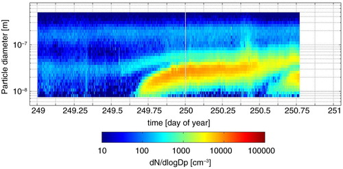
In particle number size distribution (PNSD) measurements at a fixed location, NPF often appears as a new mode of particles in the smallest measured size classes of the PNSD. After the formation of new particles has ceased, the observed mode often keeps growing, resulting in the characteristic pattern observed in time-particle size number distribution plots (Fig. 1), often referred to as a NPF banana.

Fig. 1 A banana-shaped new particle formation event observed at the Sammaltunturi measurement site in the Pallas-Sodankylä GAW station 5–6th of September 2000. The x-axis is time in day-of-year and particle number concentration in each size class is given with colour in dN/dlog₁₀ D _p.

There have been a number of studies addressing the spatial scale of NPF events. This has often been done by analysing the same NPF days at several measurement sites in the same area (Stanier et al., 2004; Komppula et al., 2006; Wehner et al., 2007; Hussein et al., 2009; Jeong et al., 2010; Crippa and Pryor, 2013) or at sites close to each other or at different altitude (Birmili et al., 2003; Boulon et al., 2011). In these studies the spatial scale of NPF has been observed to be often hundreds of kilometres, but formation and growth rates (GRs) of the particles and the timing of the event have been observed to vary from site to site within the area. Also differences between the planetary boundary layer and free troposphere and between different altitudes within the planetary boundary layer were found. Another approach has assumed simultaneous formation of particles over a large area, and used trajectories to connect the particles observed during the growth process to the location upwind of the measurement site where the air was during the particle formation (Hussein et al., 2009; Kristensson et al., 2014).

If we assume that:

1. the formation of particles takes place simultaneously over a large geographic area,

2. the NPF rates are identical at the measurement site and where the smallest observed particles were formed, and

3. all particles grow simultaneously with the same GR within the region of formation,

then advection does not impact the time evolution of the growing mode observed at the measurement site. We can calculate the particle GR from the GR of the observed particle mode (Makelä et al., 1997; Kulmala et al., 2004a), but this requires that assumptions 1 and 3 hold. The presence of particles in the lowest size class at each measurement time step requires that the formation of new particles continues at or near the site; from this we can calculate the formation time period (e.g. Asmi et al., 2011; Kristensson et al., 2014). Based on assumptions 2 and 3, the NPF rate can be calculated from the observed number concentration in the new mode. However, this also requires that the losses occurring during particle growth (from formation size to the size where they are first observed) can be quantified (Dal Maso et al., 2005). By combining the evolution of the new particle mode with trajectory data we can, based on assumption 1 and 3, calculate where the observed particles were formed between 1 and 2 nm diameter at each measurement time and get the extent of the formation area upwind of the station (Hussein et al., 2009; Kristensson et al., 2014).

To complete the analysis of NPF and growth parameters presented above one has to assume that the time-dependent formation and GR of the particles is spatially invariant. Here, we investigate how spatial variations in the formation and GRs of new particles would appear in observations of PNSDs at a fixed measurement site. The three main research questions are: (1) How do spatial variations in NPF and GRs manifest themselves in observations of NPF events? (2) Can the effects of spatial and temporal variations in formation and GRs on the observations be separated? (3) Is there more than one way to produce a specific shape of an observed NPF event?

To answer these questions we coupled a zero-dimensional aerosol box model with one-dimensional atmospheric flow to describe the impact of advection on the evolution of simulated NPF events. The structure of the model is described in Section 2. Particle formation and GRs are input parameters that can vary as a function of time and location, using wind speed to connect location to time, with output simulating measurements at a fixed location. The formation and GRs of the particle mode calculated from the simulated observations for different scenarios are presented in Section 3, and are compared with the values given as input parameters.

The model we created in this study is highly simplified, and several important aerosol processes have been excluded. This is a deliberate choice made in order to clearly separate and identify the patterns created by spatial and temporal variations in the input parameters. The purpose of the model, at its current state, is not to replicate real observations, but to demonstrate the importance of taking into account spatial changes in formation and GRs of particles in analyses of field measurement data. The creation of a more realistic model for replicating or interpreting field measurement data lies further ahead.

2. LMASON model

2.1. Structure of the model

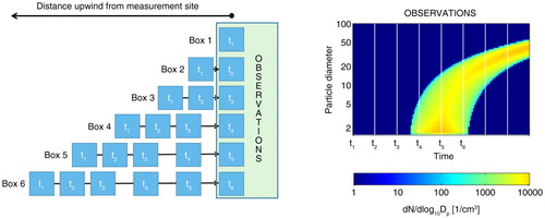
The LMASON model (Lagrangian Model for Analyzing Stationary Observations of NPF events) uses a set of aerosol box models placed along a hypothetical trajectory. These boxes are then advected along the trajectory (Fig. 2, left) and are forced by the local conditions defined for that particular location and time. The particle size distribution in each box is presented with a number of monodisperse bins. Particle number concentration and particle diameter in these bins can change due to the forcings. The PNSD from each box is recorded as they are advected over the fixed measurement location, and combined to create a plot showing the evolution of PNSD as function of time given in the right-hand panel of Fig. 2. In this study, we initialized the model with 288 boxes, and used a 10-minute time interval to simulate a 48-hour measurement.

Fig. 2 Schematic of the LMASON model. The t _i values represent the time at time step i. Note the wind speed change between t₃ and t₄ affecting the distance that the boxes move between time steps. The particle size distribution in each box as it advects over the measurement site provides the simulated observations (on the right).

2.2. Input parameters

The direct link between location and time is given by the wind speed, WS(t) through the advective transformation, so that the location of each box along the trajectory at each time point, X _(b,i), relative to the simulated measurement station, is1

where b is the index of the box, i is the index of the time step and Δt _step is the length of the time step. In LMASON the wind speed can be constant or vary as a function of time. The formation rate of new particles at 1.5 nm size [J _1.5(t,X)] is a user-defined input parameter. It is defined as2

where T _J1.5 (t) is the dimensionless temporal (time-dependent) component of J _1.5(t,X) and S _J1.5(X) is the dimensionless spatial (location-dependent) component of J _1.5(t,X).

The growth rate of particles (GR) is defined similarly to J _1.5 as:3

where T_GR(t) and S_GR(X) are, respectively, the dimensionless temporal and spatial components of GR(t,X). This GR represents the condensational growth of particles in the model.

Accounting for Brownian coagulation in the simulations is optional. Coagulation is only included as a sink of sub-150 nm particles. The model has an option for creating a coagulation sink with a pre-described monodisperse accumulation mode at 200 nm diameter. The number concentration of this mode (N ₂₀₀) is given as an input value. In the beginning of the simulation every box has this background particle mode regardless of the location of the box.

2.3. Processes

In the current version of the model there are three aerosol dynamic processes that can alter the PNSD in the moving boxes: formation of new particles with 1.5 nm diameter, condensational growth of the existing particles, and coagulation loss of particles to the background mode. Even though the input parameters and movement of the boxes are treated with 10-min time steps, the aerosol dynamic processes are simulated with 1-minute time step, Δt _dyn, for better numerical accuracy, especially in the early stages of particle growth. PNSD in each box is presented with a varying number of monodisperse particle bins with changing diameter. The only process affecting the number of particles in an individual bin is scavenging of the particles by coagulation. Other processes can be included in the model, but are intentionally excluded in this study in order to highlight the effect of spatio-temporal variations in the formation and growth parameters.

As described in the previous section, formation of new particles is a user-defined parameter. This means that for each box at each time step there is a value for J _1.5(t,X). If this J _1.5(t,X)>0, a new monodisperse particle bin is created at a diameter of 1.5 nm. The number of particles in this bin is given by J _1.5(t,X)×Δt _dyn. No particles are added to pre-existing bins due to NPF. Initially, there is only one bin in each box: the background population of 200 nm particles. The upper limit of the number of particle bins in a given box is defined by the number of Δt _dyn for that box during the model run. This case represents the case of continuous NPF everywhere along the trajectory of the box.

The condensational growth of the particles is simulated using the full-moving method (Korhonen et al., 2004; Jacobson, 2005), where the particles grow to their exact size without numerical diffusion, by simply increasing the diameter of each bin in the box by GR(t,X)×Δt _dyn. This applies only to particles with diameter D _p<150 nm and particles larger than this are not allowed to grow, which forces the coagulation sink to be kept constant through the simulation (again, deliberately selected to exclude effects other than spatio-temporal variation in the formation and growth parameters). The condensational growth is calculated in each Δt _dyn after the potential NPF.

The coagulation losses for each particle size bin are calculated after the condensational growth. Because coagulation is only treated as a sink for particles, the diameters of the bins do not change and no new bins are created due to coagulation. With this approach, coagulation impacts only the particle number concentration in each bin. For a more detailed description of the different methods for dynamical modelling of particle size distribution see, e.g. Korhonen et al. (2004), Jacobson (2005) or Roldin et al. (2011).

2.4. Output of the model

As air parcels advect past the hypothetical measurement site (at location X=0), the PNSD is fitted to a fixed size grid with bins distributed equally on a logarithmic scale, and presented as dN/dlog₁₀(D _p). The fitting is conducted in a way that conserves the particle mass and number concentration, but causes a slight broadening of the size distribution (Korhonen et al., 2004). The model stores this PNSD in each box at X=0. These PNSDs and the total particle number concentration as a function of time are saved in the output file, representing real atmospheric measurements at a fixed-point measurement site.

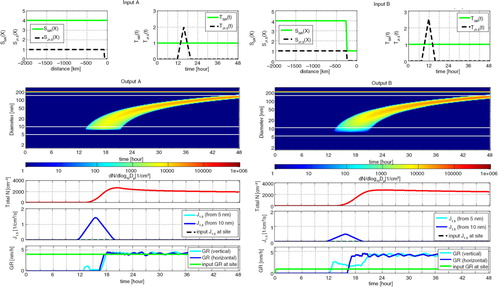
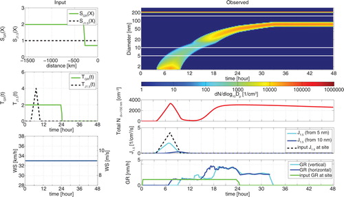
The particle formation rate at 1.5 nm is calculated from the PNSD at a hypothetical fixed-point measurement site using the revised Kerminen-Kulmala equation (Lehtinen et al., 2007). In this study, this calculation utilises particle number concentrations at 5 and 10 nm. The calculation is not exact because neither the Kerminen-Kulmala equation nor the handling of coagulation in the model is exact, therefore a perfect match with the input J _1.5(t,X) is not expected. The GR of particles is calculated from the data using two methods, one following the peak of the mode as a function of time (similar to Dal Maso et al., 2005) and the other following the time at which the maximum particle number concentration is reached at each size bin (Lehtinen and Kulmala, 2003). The output data is converted to dN/dD _p from dN/dlog₁₀ D _p when calculating the GRs as presenting the size distribution on logarithmic diameter axis has been shown to cause error in the GR determined by following the peak of the mode (Leppä et al., 2011). A plot presenting the PNSDs as a function of time at X=0 is generated, together with outputs describing the evolution of total number concentration of particles with D _p<150 nm as a function of time, particle formation rate and GR of the observed mode at the station, and the corresponding J _1.5(t,0) and GR(t,0) calculated from the input parameters ( Fig. 3). The input parameters of WS, T _J1.5(t), S_J1.5(X), T_GR(t) and S_GR(X) are also included in the figure.

Fig. 3 Plot of a new particle formation event provided by the LMASON model output. This event is only limited temporally [T_J1.5(t)>0 between hours 8 and 16, all other parameters are constant]. Panels on the left show the input values for S_J1.5(X) and S_GR(X) (top), T_J1.5(t) and T_GR(X) (middle) and WS (bottom). On the right, the top panel shows the evolution of the particle number size distribution (PNSD) as a function of time over 2 days, with particle number concentrations in each bin given as colour in dN/dlog₁₀ D _p. The second panel shows the number concentration of particles with D _p<150 nm as a function of time. The third panel shows the formation rate, J _1.5, as calculated from the output PNSD data and compared to the input values. The lowest panel shows particle growth rates as a function of time calculated from the output PNSD data using mode peak diameter at each time point (vertical) and times of maximum particle number concentration in each size class (horizontal), and the input growth rate at the measurement site as a function of time.

2.5. Limitations of and excluded processes from LMASON

The LMASON model is highly simplified. This is a deliberate choice made in order to focus on the different impacts that spatial and temporal variations in the formation and growth parameters have, without masking them with other effects. This, however, leads to a number of limitations for the model's ability to simulate real atmospheric processes shaping the PNSD. The main limitations are discussed below.

The method used to combine the spatial and temporal parameters is quite simple, limiting the possible spatio-temporal patterns that can be simulated. Any spatial patterns in the model input will affect all temporal patterns and vice versa. Setting up the spatial and temporal patterns simultaneously would make them independent of each other, and allow simulations where some temporal patterns apply only on some parts of the upwind area. The current way of inputting the parameters is, however, enough for this initial study.

The current version of the model assumes that all air masses advecting past the station follow the same trajectory, so that any changes in the input parameters are identical along all trajectories. This is not true in the real world and it limits the number of real NPF events that can be simulated with LMASON. Including the changing trajectories would clearly improve the model applicability, but it would also complicate the input of the formation and growth parameters.

The model assumes the air to be in a vertically perfectly mixed boundary layer at all times leading to modelled air parcels being affected by NPF instantaneously regardless of the altitude in which the formation occurs. This prevents the model from accounting for altitude dependence of particle formation and GRs (Birmili et al., 2003; Wehner et al., 2007; Boulon et al., 2011).

The background aerosol population, and thereby coagulation sink, does not change as a function of time or location. Observations typically show a drastic decrease in the background particle concentration due to the growth of the boundary layer height in the morning just before NPF occurs (Nilsson et al., 2001). This effect cannot be simulated with the current version of LMASON.

The structure of the model, a set of advecting boxes that are simulated independently, currently precludes any horizontal mixing between the boxes. Physically, the limitations mean that there is no turbulence, no compression of air and no frictional force imparted by surface type or topography, with all air in the boundary layer assumed to advect along the trajectory with the same speed.

There are also a number of other processes excluded, but these do not limit the usability of LMASON as much as the five mentioned above. Because of these limitations, the current form of LMASON can be used to interpret real measurement data only in specific cases. It is, however, a powerful tool for studying the combined effects of spatially and temporally varying formation and GRs of new particles, and to explore the importance of taking spatial variability into account in NPF event analysis.

3. Results

3.1. Distance of no information

If the measurements do not extend down to the sizes at which particles are actually formed, we cannot obtain information on the particles with diameter below the detection limit diameter. This prevents us from observing particles that form so near the observation site that they advect past the site before they reach the detection limit diameter. This creates a ‘distance of no information’ upwind of the station. This distance (X ₀) depends on the lowest detectable particle size (D _p,min) in the measurements, particle GR and the advection speed (=wind speed, WS):4

If we assume the GR to be size-dependent and to have smaller values at smaller particle diameter (Kulmala et al., 2004b), the distance of no information is longer. Beyond this distance we can only observe any newly formed particles if they survive to the measurement site without being scavenged by coagulation.

3.2. Particle formation

It is possible to distinguish between temporally limited and spatially limited NPF. If the formation of new particles is limited only temporally, we can detect a clear continuous NPF banana at the observation site (Fig. 3, upper right panel). From that banana we can also calculate the time-dependent formation rate of new particles (Figs. 3, 3rd right panel) and the growth of the observed new mode (GR(t)_obs, Fig. 3, bottom right panel). If formation of new particles is limited only spatially (formation taking place continuously within a limited area upwind of the site) the new mode of particles appears as a layer in the plot showing the evolution of PNSD at the observation site (Fig. 4, upper right panel). The diameter range of this layer can vary if T_GR(t) or WS(t) varies. If formation of new particles is limited to a specific time window and to a specific area, the observations show a section of an NPF banana cut horizontally at certain particle diameters (Fig. 5). These diameters depend on GR(t,X), WS and distance between the observation site and the edge of the formation area (X) as5

Fig. 4 New particle formation limited spatially only [constant T_J1.5(t)] taking place 200–400 km upwind of the measurement site) starting at t=0. The figure panels are the same as in Fig. 3.

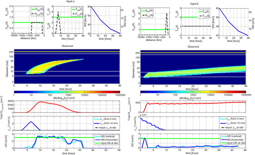
Fig. 5 Two very similar simulated observations from different input conditions. The figure explanations are as in Fig. 3. (a) shows new particle formation taking place between hours 12 and 20 more than 70 km upwind of the measurement site. Particle growth rate is constant and wind speed is constant 50 km h⁻¹. (b) shows new particle formation taking place between hours 8 and 16 more than 270 km upwind of the measurement site. Particle growth in the closest 270 km is lower than that beyond this limit. Wind speed is again constant 50 km h⁻¹.

where D _p,cut is the particle diameter where the cut occurs. If the area of particle formation extends near the measurement site, but does not include the site, it is possible that the lower cut-off limit of the banana is below the lowest detectable particle size. In the cases presented in Fig. 5, a formation rate can be calculated from the number concentration of 10 nm particles, even though there is no NPF taking place at the measurement site. If the lowest measured particle size was 10 nm, the edge of the formation area would be within the distance of no information, and the formation could be falsely assumed to be taking place at the site.

Figure 5 also demonstrates that when there is no mode to follow down to the sizes at which the particles are formed, there is not enough information to infer what happens to particles in the missing size range and in the respective area upwind of the measurement site. This lack of information can result either from the lowest measurable particle diameter being too large or from no NPF taking place near the site. Figure 5a and b show two very similar looking NPF events that were created using two quite different sets of input parameters, including different formation times, formation areas and growth areas. This means that the same specific shape of an observed NPF event can be produced in more than one way.

3.3. Particle diameter growth

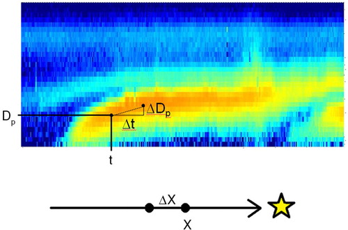
The size of particles observed at a fixed measurement site is the result of all growth [integral of GR(t,X)] between the formation and observation of the particles, regardless of whether the growth depends on time, location, or both. From measurements conducted at a fixed location, an apparent GR [GR(t)_obs] of the growing mode as a function of time can be calculated from the time dependency of the particle diameter of the mode. This is done as (Fig. 6), where Δt is the difference between two time points and ΔD _p is the corresponding change in the peak diameter of the mode. As D _p is affected by both T_GR(t) and S_GR(X), the observed GR, GR(t)_obs, only corresponds to the real T _GR(t) at the measurement site if S_GR(X) throughout the formation area is the same as S _GR(0), i.e. the value at the measurement site. At the other extreme, if we assume T_GR(t) to be constant, GR(t)_obs between two sets of particles observed at different points of time depends only on S _GR(X) between the locations where these two sets of particles were formed. The particles observed at times t and t+Δt are formed at distances X and X+ΔX upwind of the measurement site, respectively (Fig. 6). If T _GR (t) is constant, both sets of particles experience exactly the same growth between X and the measurement site. As a consequence, the observed difference in ΔD _p, and thereby GR(t)_obs between times t and t+Δt, can only be caused by particle growth at the distance ΔX located somewhere upwind of the measurement site. In such cases, a section of increased GR(t)_obs in the observed banana is a manifestation of an area with increased S_GR(X) at the time of particle formation upwind of the site (Fig. 6), and does not represent what is happening at the measurement site. We can calculate this distance X by6

Fig. 6 The change of peak particle diameter ΔD_p of the growing mode between times t and t+Δt extracted from an observed new particle formation event, and the corresponding change in location where the observed particles were formed ΔX along a trajectory upwind of the measurement site (marked with a star). The new particle formation event in the figure is the same one as in Fig. 1.

where t _form is the time when formation of new particles is observed. This information might not always be available, as there might be no NPF occurring at the measurement site. If GR(t,X) is truly varying as a function of both t and X, the observed GR, GR(t)_obs, is a combination of these two cases. Beyond these effects, GR(t)_obs can also differ from the GR of the individual particles due to coagulation scavenging, which removes smaller particles more efficiently (Stolzenburg et al., 2005).

In our simplified model, the effects that temporal and spatial changes in input GR have on GR(t)_obs can be separated. Temporal changes [changes only in T_GR(t)] result in a change in GR(t)_obs occurring in all size classes at the same time (Fig. 7, upper right panel). This also means that the width of the mode on the diameter axis remains unchanged, and there is no sudden change in the particle number concentration. The GR calculated from the output data also corresponds to the particle GR at the measurement site.

Fig. 7 A new particle formation event with temporal changes in particle growth rate at hours 16 and 32 [T _GR(t) changing, S _GR(X) constant]. The figure explanations are as in Fig. 3.

In case of a change in S _GR(X), the change in GR(t)_obs happens to all particles at the same diameter, but not at the same time. In such case the width of the mode on the time axis remains unchanged, but the diameter width of the mode changes proportionally to the change in S_GR(X). This can be seen in Fig. 8 (at t=14 hours to t=20 hours), where the diameter width of the mode is about 10 nm at t=12 hours, and about 25 nm at t=21 hours. The latter particles were formed where S_GR(X)=2, the earlier where S_GR(X)=0.75. Also the total number concentration is altered, because within the area of higher GR a larger fraction of the particles survives through the sizes where coagulation is most efficient, and are therefore observed at the measurement site. This means that the total number concentration in the observed banana (N _{Dp<150 nm}) as a function of time can vary even though the formation rate of new particles does not change. The relative change in observed N _{Dp<150 nm} can be higher or lower than that in S_GR(X), depending on how large a fraction of the newly formed particles are removed by coagulation. In extreme cases, coagulation can scavenge all particles formed at a certain area upwind of the measurement site (Kerminen et al., 2001), meaning that not only a varying S_J1.5(X), but also a varying S_GR(X) can lead to situations where some parts of the banana are entirely missing.

Fig. 8 A new particle formation event where growth rate changes as a function of location (from t=14 to t=20 hours) and as a function of time (at t=24 hours). Notice the observable growth continuing after 24 hours, even though GR(t,X)=0.

If particle GR changes as a function of both time and location, observable growth GR(t)_obs can continue even in time periods where T_GR(t)=0, meaning that there is no growth taking place anywhere in the model domain. This is demonstrated in the case presented in Fig. 8. The particles do not grow after t=24 hours, meaning that all particle growth has taken place between the formation time (from t=4 hours to t=10 hours) and the time of termination of growth (t=24 hours). After this, particles arriving at the measurement site later have spent longer time in the high growth area compared to those arriving earlier at around t=24 hours. The observable positive GR GR(t)_obs between t=24 hours and t=32 hours is caused by the difference in S_GR(X) between the area up to 300 km upwind of the site and the locations further away. After t=32 hours, all particles advecting over the measurement site have experienced their entire growth in the area of higher GR, and no more growth is observed. This phenomenon demonstrates that GR(t)_obs and the real growth of the particles can behave very differently in certain situations.

3.4. Effect of wind speed changes on observable evolution of PNSD

All of the effects described in Sections 3.1–3.3 were simulated with constant wind speed. A lower wind speed results in particles formed within a certain area taking longer to arrive at the measurement site. This means that the particles have had a longer time to grow and reach larger diameters by the time they are observed at the site. In a temporally limited NPF event the GR(t)_obs is not affected, because the time at when the particles arrive at the site is also shifted. If wind speed varies as a function of time, any location-dependent changes do not take place at the same diameter for all particles, so that the particle diameter at which the change occurs is a function of time (Fig. 9a, 2nd panel from top). In the case of a spatially limited event [constant T_J1.5(t)] the entire diameter range in which the particles appear at the measurement site varies as function of time. In some cases, such a layer of increasing particle size can be misinterpreted as a NPF banana (Fig. 9b, 2nd panel from top) giving false formation rate, time and area, as well as false GRs. Those meteorological parameters that directly affect the formation or GRs of the particles at a given time and/or location can be simulated by changing the input values of the model, and are not discussed here.

Fig. 9 How changes in wind speed affect observations of different new particle formation events. The figure explanations are as in Fig. 3. (a) shows a spatially and temporally limited new particle formation event with decreasing wind speed and (b) shows a spatially limited new particle formation event with decreasing wind speed, resulting in a ‘false banana’.

4. Case study: negative GR observed in measurements

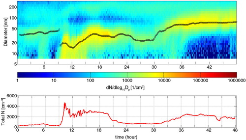
NPF has been monitored at the Pallas-Sodankylä GAW station since 2000 (Asmi et al., 2011). There have been a number of cases when the GR(t)_obs has been negative at some point during a NPF event (Fig. 10). The decrease in the diameter of the particle mode is more than can be explained by instrumental uncertainty (Wiedensohler et al., 2012). If this was to be explained only through temporal changes in GR, it would require particles to decrease in size. This necessitates either the collapse of structured particles or evaporation of material from the particles into the surrounding air. Both of these explanations are unlikely because freshly formed particles are assumed to be close to spherical and to consist of compounds with very low vapour pressure (Kulmala et al., 2004a and references therein).

Fig. 10 An observed new particle formation event at the Sammaltunturi site in Pallas-Sodankylä GAW station 15–16th of July 2011. The black circles represent the evolution of particle diameter (1-hour sliding average of diameter of the size bin with highest particle concentration in dN/dlog₁₀ D _p). A period of mostly decreasing particle size can be seen between hours 17 and 30.

Allowing for spatial variation in the growth parameters provides a more plausible explanation of observed negative growth, with the situation in Fig. 11 being the counterpart to the conditions in Fig. 8. If T_GR(t) becomes zero or close to zero at some time point t*, all formed particles that arrive at the measurement site after t* have had roughly the same amount of time to grow. If S_GR(X) is significantly higher near the measurement site than further away, then the particles arriving at the site later have spent a larger fraction of their growth time in the area with low S_GR(X), and therefore are smaller when observed at the site.

Fig. 11 Simulation of the observed event presented in Fig. 10 using both a temporally and spatially varying growth rate. Figure explanations are as in Fig. 3. The yellow line in the upper right panel is the evolution of the peak diameter in Fig. 10.

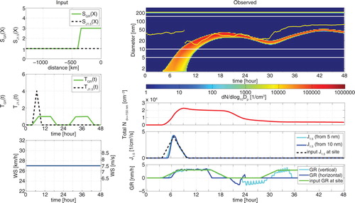
To test this approach we analysed the air masses arriving at the Sammaltunturi measurement site in the Pallas-Sodankylä GAW station on July 15–16th 2011 using the online version of HYSPLIT trajectory model (Draxler and Hess, 1998), using back-trajectories from an altitude of 300 m above ground level. During the NPF event presented in Fig. 10, the air mass was arriving from west during the entire event, with wind speeds varying between 20 and 35 km h⁻¹ near the site. For simulating the same event (Fig. 11) we used a constant wind speed of 27 km h⁻¹. The terrain west of the Sammaltunturi site consists of boreal forest for the first 200 km, then subarctic birch forest and mountain tundra at higher altitudes for the next 100–150 km, and then changes to the North Atlantic Ocean at about 350–400 km west from the site. In our simulation of this event we have assumed that particle GR over the land areas is three times as high [S_GR(0 km<X<350 km)=3] as that over the ocean [S_GR(X>400 km)=1]. These GR values are roughly in line with typical values measured at Pallas (Asmi et al., 2011; Väänänen et al., 2013) and over Northern Atlantic and Arctic Oceans (O'Dowd et al., 2010; Karl et al., 2012). We defined the simulated time period to start at midnight. We assumed a diurnal cycle in the GR, being zero at night, and a NPF event taking place everywhere in the domain between t=4 hours and t=10 hours. With these justifiable values we were able to simulate the time evolution off PNSD (Fig. 11) very similar to what was observed on July 15–16th 2011 at Sammaltunturi (Fig. 10). Both the real observations and the simulated ones show a new particle mode appearing in the first morning and to reach the size of 7 nm around 7 hours<t <8 hours. The observed particle mode grows to roughly 30 nm diameter by t=18 hours in the afternoon, after which the mode diameter decreases to 20 nm by the next morning. In the morning of the second day the diameter of the new particle mode starts to increase again. Even though the simulated particle number concentration exceeds the measured one significantly, both number concentrations show very similar decrease at t=21 hours in the first evening.

5. Conclusions

The LMASON model was created for studying the effects of spatially and temporally varying formation and growth parameters on observations of NPF events at fixed measurement sites. In the model the user may input the particle formation and GRs as functions of both time and distance upwind from a hypothetical measurement site. The user can also describe the advection (wind speed) as a function of time. The output of the model is the time evolution of the PNSD at the measurement site, simulating real measurements of air advected past a fixed location. The model is highly simplified, and several processes that also modify the particle size distribution are left out in order not to mask the effects of interest.

For the LMASON results presented in this study, the temporal and spatial changes in GR were distinguishable from each other. A temporal change occurs at the same time in all size classes and does not affect the particle number concentration. A spatial change affects all particles when they reach a certain diameter. This leads to widening or narrowing of the new mode as well as to a change in the particle number concentration, because the particle GR where the particles are small is an important factor defining how large fraction of the particles survive to the measurement site. In reality, these changes do not typically occur stepwise but smoothly, which would make it much harder to distinguish whether a change in GR(t)_obs depends more on time or particle diameter. If there are no other processes that modify the size distribution, such as changes in boundary layer height, coagulation sink or air mass trajectory route, simultaneous changes in GR(t)_obs and N of the new mode in a NPF banana after the formation of new particles have ceased can reveal information about the effect causing the change (Table 1).

Table 1. Effects of doubling different input parameters on the observable parameters of the growing mode at the measurement site in a temporally limited (‘banana type’) NPF event

Changing parameter	Change in GR(t)obs of the mode	Change in N Dp<150 nm of the mode	Change in diameter width of the mode
2×S J1.5(X) upwind	No effect	2×	No clear effect
2×TGR(t)	2×	No clear effect	No clear effect
2×SGR(X) upwind	2×	Increase	2×

The effects are described as if they occur in the observable data after the formation of new particles has ceased. The direction of the spatial changes is towards upwind of the site.

The variations in the particle number concentration and particle GR that we observe can be explained with either temporal or spatial variations in the formation and growth parameters, or a combination of the two types. When there are several changes occurring simultaneously, separating them becomes more complicated. We have also shown that it is possible to produce very similar simulated observations with more than one set of input parameters. In other words, inferring any of those parameters from observed time evolution of particle size distribution is ambiguous.

If a change in the observed particle number concentration or GR is caused by spatial variations upwind of a measurement site, connecting it to temporal changes of other parameters, such as concentrations of potential precursor gases for particle growth, measured at the site, can easily lead to false conclusions. Furthermore, if the particle size distribution measurements do not extend down to the size where the particles form, we cannot conclude whether the site is within the area where new particles are formed or not. Changes in particle GR near the measurement site can also be missed if the minimum measureable size is too large. In such cases, analysis of the measurements may yield an incorrect particle formation rate and formation time period, as well as an incorrect GR. In extreme cases, variations in the advection speed can lead to a situation where even the type of event (spatially or temporally limited formation) can be misinterpreted. We conclude that the standard analysis of PNSD data only at a fixed measurement site does not contain enough information to characterise the NPF event in a controlled manner. In some cases with spatially varying parameters it can lead to incorrect formation rate, formation time, formation area, GR, time dependency of growth and even the type of event.

A trajectory analysis combined with the formation and GR analysis can aid in understanding the observed event, and can help to decide whether time-dependent or location-dependent change in parameter values is a more plausible scenario. Relatively homogenous terrain upwind of a measurement site can help justify the assumption that the observed changes are mainly temporal in nature, and the further the homogenous area extends upwind of the site, the further the assumption can be extended. For less speculative analyses, it appears that the same air parcel should be measured at more than one location (e.g. Väänänen et al., 2013) or that an air parcel should be trapped in a chamber so that the growth of the particles can be followed at the site without effects of advection (e.g. Bonn et al., 2013).

5.1. Future research

There are several steps for developing the LMASON model further. Of major importance is making the input of spatial and temporal parameters truly independent of each other, allowing a more flexible use of the model in simulating different scenarios. A second measurement site upwind of the first one in the model domain would also bring a lot of new possibilities when analysing NPF in air masses advecting over multiple measurement sites (e.g. Komppula et al., 2006; Väänänen et al., 2013). This would allow a stronger separation of temporal and spatial effects in real observations of NPF events, and further make a measurement-based verification of spatially changing parameters feasible.

It is planned to make the model two- or three-dimensional in the future so that it can be more realistically applied to a wider range of observed NPF events. This means, however, that the user-defined input parameters would be functions of time, longitude, latitude and potentially altitude simultaneously, yet independently. The air mass trajectories would also need to be time-dependent. An alternative option is to include the approach of this model in a pre-existing and more advanced air mass transport model, which already has the three-dimensional approach.

Additional improvements such as a changing background particle mode, dry and wet deposition of particles, and intramodal coagulation are planned to be included in the next stage of model development.

6. Acknowledgements

This work was supported by the Academy of Finland through The Centre of Excellence in Atmospheric Science – From Molecular and Biological processes to The Global Climate, the Nordic top-level research initiative CRAICC (Cryosphere–atmosphere interactions in a changing Arctic climate), and by the Maj and Tor Nessling Foundation. The study is also a contribution to the Lund University Strategic Research Areas: Modeling the Regional and Global Earth System (MERGE). J. Leppä would like to acknowledge the funding received from the Magnus Ehrnrooth Foundation, the Jane and Aatos Erkko Foundation and the Emil Aaltonen Foundation. P. Roldin would like to acknowledge the Swedish Research Council for Environment, Agricultural Sciences and Spatial Planning FORMAS (Project No. 214-2014-1445).

References

- Asmi E. , Kivekäs N. , Kerminen V.-M. , Komppula M. , Hyvärinen A.-P. , co-authors . Secondary new particle formation in Northern Finland Pallas site between the years 2000 and 2010. Atmos. Chem. Phys. 2011; 11: 12959–12972.
- Birmili W., Berresheim H., Plass-Dülmer C., Elste T., Gilge S., co-authors. The Hohenpeissenberg aerosol formation experiment (HAFEX): a long-term study including size-resolved aerosol, H2SO4, OH, and monoterpenes measurements. Atmos. Chem. Phys. 2003; 3: 361–376. http://dx.doi.org/10.5194/acp-3-361-2003.
- Bonn B., Sun S., Haunold W., Sitals R., van Beesel E., co-authors. COMPASS – COMparative particle formation in the atmosphere using portable simulation chamber study techniques. Atmos. Meas. Tech. 2013; 6: 3407–3423. http://dx.doi.org/10.5194/amt-6-3407-2013.
- Boulon J., Sellegri K., Hervo M., Picard D., Pichon J.-M., co-authors. Investigation of nucleation events vertical extent: a long term study at two different altitude sites. Atmos. Chem. Phys. 2011; 11: 5625–5639. http://dx.doi.org/10.5194/acp-11-5625-2011.
- Crippa P. , Pryor S. C . Spatial and temporal scales of new particle formation events in eastern North America. Atmos. Environ. 2013; 75: 257–264.
- Dal Maso M. , Kulmala M. , Riipinen I. , Wagner R. , Hussein T. , co-authors . Formation and growth of fresh atmospheric aerosols: eight years of aerosol size distribution data from SMEAR II, Hyytiälä, Finland. Boreal Environ. Res. 2005; 10: 323–336.
- Draxler R. R. , Hess G. D . An overview of the HYSPLIT_4 modeling system of trajectories, dispersion, and deposition. Aust. Meteor. Mag. 1998; 47: 295–308.
- Hussein T. , Junninen H. , Tunved P. , Kristensson A. , Dal Maso M. , co-authors . Time span and spatial scale of regional new particle formation events over Finland and Southern Sweden. Atmos. Chem. Phys. 2009; 9: 4699–4716.
- Jacobson M. Z . Fundamentals of Atmospheric Modelling. 2005; Cambridge, United Kingdom: Cambridge University Press. 2nd ed ISBN: 0 521 54865 9.
- Jeong C.-H. , Evans G. J. , McGuire M. L. , Chang R. Y.-W. , Abbatt J. P. D. , co-authors . Particle formation and growth at five rural and urban sites. Atmos. Chem. Phys. 2010; 10: 7979–7995.
- Karl M., Leck C., Gross A., Pirjola L. A study of new particle formation in the marine boundary layer over the central Arctic Ocean using a flexible multicomponent aerosol dynamic model. Tellus B. 2012; 64: 17158. http://dx.doi.org/10.3402/tellusb.v64i0.17158.
- Kerminen V.-M., Lihavainen H., Komppula M., Viisanen Y., Kulmala M. Direct observational evidence linking atmospheric aerosol formation and cloud droplet activation. Geophys. Res. Lett. 2005; 32: L14803. http://dx.doi.org/10.1029/2005GL023130.
- Kerminen V.-M. , Pirjola L. , Kulmala M . How significantly does coagulational scavenging limit atmospheric particle production?. J. Geophys. Res. 2001; 125: 24110–24125.
- Komppula M. , Sihto S.-L. , Korhonen H. , Lihavainen H. , Kerminen V.-M. , Kulmala M. , Viisanen Y . New particle formation in air mass transported between two measurement sites in Northern Finland. Atmos. Chem. Phys. 2006; 6: 2811–2824.
- Korhonen H., Lehtinen K. E. J., Kulmala M. Multicomponent aerosol dynamics model UHMA: model development and validation. Atmos. Chem. Phys. 2004; 4: 757–771. http://dx.doi.org/10.5194/acp-4-757-2004.
- Kristensson A. , Johansson M. , Swietlicki E. , Kivekäs N. , Hussein T. , co-authors . NanoMap: geographical mapping of atmospheric new-particle formation through analysis of particle number size distribution and trajectory data. Boreal Env. Res. 2014; 19(Suppl B): 329–342.
- Kulmala M., Kontkanen J., Junninen H., Lehtipalo K., Manninen H. E., co-authors. Direct observations of atmospheric aerosol nucleation. Science. 2013; 339: 943–946. [PubMed Abstract].
- Kulmala M., Laakso L., Lehtinen K. E. J., Riipinen I., Dal Maso M., co-authors. Initial steps of aerosol growth. Atmos. Chem. Phys. 2004b; 4: 2553–2560. http://dx.doi.org/10.5194/acp-4-2553-2004.
- Kulmala M., Vehkamäki H., Petäjä T., Dal Maso M., Lauri A., co-authors. Formation and growth rates of ultrafine atmospheric particles: a review of observations. J. Aerosol Sci. 2004a; 35(2):143–176. DOI: http://dx.doi.org/10.1016/j.jaerosci.2003.10.003.
- Lehtinen K. E. J., Dal Maso M., Kulmala M., Kerminen V.-M. Estimating nucleation rates from apparent particle formation rates and vice versa: revised formulation of the Kerminen–Kulmala equation. J. Aerosol Sci. 2007; 38(9):988–994. DOI: http://dx.doi.org/10.1016/j.jaerosci.2007.06.009.
- Lehtinen K. E. J. , Kulmala M . A model for particle formation and growth in the atmosphere with molecular resolution in size. Atmos. Chem. Phys. 2003; 3: 251–257.
- Leppä J. , Anttila T. , Kerminen V.-M. , Kulmala M. , Lehtinen K. E. J . Atmospheric new particle formation: real and apparent growth of neutral and charged particles. Atmos. Chem. Phys. 2011; 11: 4939–4955.
- Makelä J. M. , Aalto P. , Jokinen V. , Pohja T. , Nissinen A. , co-authors . Observations of ultrafine aerosol particle formation and growth in boreal forest. Geophys. Res. Lett. 1997; 24: 1219–1222.
- Nilsson E. D. , Rannik Ü. , Kulmala M. , Buzorius G. , O'Dowd C. D . Effects of continental boundary layer evolution, convection, turbulence and entrainment, on aerosol formation. Tellus B. 2001; 53: 441–461.
- O'Dowd C. D., Monahan C., Dall'Osto M. On the occurrence of open ocean particle production and growth events. Geophys. Res. Lett. 2010; 37(19):L19805. DOI: http://dx.doi.org/10.1029/2010GL044679.
- Riipinen I., Yli-Juuti T., Pierce J. R., Petäjä T., Worsnop D. R., co-authors. The contribution of organics to atmospheric nanoparticle growth. Nat. Geosci. 2012; 5: 453. DOI: http://dx.doi.org/10.1038/ngeo1499.
- Roldin P., Swietlicki E., Schurgers G., Arneth A, Lehtinen K. E. J., Boy M., Kulmala M. Development and evaluation of the aerosol dynamics and gas phase chemistry model ADCHEM Atmos. Chem. Phys. 2011; 11: 5867–5896. doi: http://dx.doi.org/10.5194/acp-11-5867-2011.
- Stanier C. , Khlystov A. , Pandis S . Ambient aerosol size distributions and number concentrations measured during the Pittsburgh Air Quality Study (PAQS). Atmos Environ. 2004; 38: 3275–3284.
- Stolzenburg M. R., McMurry P. H., Sakurai H., Smith J. N., Mauldin R. L., III, co-authors. Growth rates of freshly nucleated atmospheric particles in Atlanta. J. Geophys. Res. 2005; 110: D22S05. DOI: http://dx.doi.org/10.1029/2005JD005935.
- Väänänen R. , Kyrö E.-M. , Nieminen T. , Kivekäs N. , Junninen H. , co-authors . Analysis of particle size distribution changes between three measurement sites in northern Scandinavia. Atmos. Chem. Phys. 2013; 13: 11887–11903.
- Wehner B. , Siebert H. , Stratmann F. , Tuch T. , Wiedensohler A. , co-authors . Horizontal homogeneity and vertical extent of new particle formation events. Tellus B. 2007; 59: 362–371.
- Wiedensohler A. , Birmili W. , Nowak A. , Sonntag A. , Weinhold K. , co-authors . Mobility particle size spectrometers: harmonization of technical standards and data structure to facilitate high quality long-term observations of atmospheric particle number size distributions. Atmos. Meas. Tech. 2012; 5: 657–685.