Aerosol data assimilation and forecasting experiments using aircraft and surface observations during CalNex

Abstract

Observing system experiments are presented to characterise impacts of surface and vertical profile measurements on aerosol analysis and forecast skill. A three-dimensional (3D) variational data assimilation system is implemented within the Weather Research and Forecasting/Chemistry model, and the control variables consist of eight species of the Model for Simulation Aerosol Interactions and Chemistry scheme. In the experiments, the 3D profiles of aircraft speciated observations and surface concentration observations acquired during the California Research at the Nexus of Air Quality and Climate Change field campaign are assimilated. The data assimilation experiments are performed at 02:00 local time 2 June 2010, and surface observations at 02:00 and aircraft observations from 01:30 to 02:30 local time are assimilated. The results show that the assimilation of both aircraft and surface observations improves the subsequent forecasts. The improved forecast skill resulting from the assimilation of the aircraft profiles persists a time longer than the assimilation of the surface observations, which suggests the necessity of vertical profile observations for extending aerosol forecasting time.

• aerosol data assimilation
• aircraft speciated observation
• observing system experiments
• WRF/Chem

1. Introduction

Data assimilation has been increasingly used to improve aerosol prediction in recent years in association with both global models (e.g., Zhang et al., 2008; Benedetti et al., 2009, Mangold et al., 2011) and regional models (e.g., Denby et al., 2008; Tombette et al., 2009; Pagowski et al., 2010; Liu et al., 2011; Li et al., 2013). Data assimilation aims to integrate all available observations into a model to produce optimal estimates of aerosol fields, and then used to initialise the model to improve the subsequent forecast. The development of aerosol data assimilation hinges on advancements in both aerosol models and observing networks.

Although a variety of advancements in aerosol data assimilation have been made, it is still fair to say that it is in a nascent stage, in contrast to the application in meteorology and oceanography (e.g., Kalnay, 2010; Bocquet et al., 2015). Using aerosol data assimilation to improve forecasts and particularly to extend the time of skilful forecasts continues to remain a challenge. For regional models, the improved skill sharply declines within the first 6-12 hours after the forecasting model is initialised using data assimilation analysis, although a limited positive impact of data assimilation on forecasts may persist beyond 24 hours. This paper aims to improve our understanding of the skill loss related to observations with a regional model.

The quick loss of the improved forecast skill may be related to uncertainties in surface fluxes (emission sources), dynamic properties of aerosol variability, model performance, and data assimilation performance. We hypothesise three major causes that can give rise to this decline in forecast skill. The first is related to the scarcity of aerosol measurements. Currently available aerosol observations are inadequate to determine accurate and dynamically consistent aerosol fields, thus resulting in uncertainties in the initialisation of a high-resolution forecasting model (e.g., Li et al., 2013). Further, the limited lifetime of the aerosols can reduce the impact of the initialisation on persistency of skilful forecast. The shorter lifetime the aerosol has, the less persistent impact the initialisation imposes. The second is related to emission sources. Emissions often consist of point and line sources, giving rise to small-scales in aerosol fields. The small-scales then limit the predictability of aerosol fields. And the third is related to the sensitivity of aerosol forecasts to meteorological fields. That is, the emission sources results in the sensitivity of aerosol forecasts to wind directions. These three possible causes on the quick decline in forecast skill should be characterised. It is beyond the scope of this paper to address all the three causes, but we discuss here some aspects related to inadequacy of aerosol observations.

The inadequacy of aerosol observations continues to be a challenge in aerosol data assimilation. This is primarily due to the high cost of measurements and the large number of aerosol state variables. A sophisticated aerosol model may explicitly treat more than a dozen species, and each species involves different size bins, which increase the number of state variables in multiples. A large number of state variables require a large number of observations in data assimilation. The last decade has witnessed great progress in the technology of aerosol measurement, leading to the establishment of a variety of observation networks (e.g., Diner et al., 2004). However, there are still only a few hundred aerosol measuring surface stations in the United States, and the measurements are limited to the total concentration of surface PM_2.5 or PM₁₀. There are only a few supersites measured for the detailed aerosol species (Weber et al., 2003). Instrumented-aircraft measurements, which often provide aerosol profiles, are even more limited in space and time (Morgan et al., 2009). Satellite measurements provide global coverage, but the most common observations are aerosol optical depths (AODs) and are often unavailable due to clouds and high surface reflectance (van Donkelaar et al., 2010; Levy et al., 2010; Lee et al., 2011). A global lidar network has been established to measure aerosol scattering profiles but is limited to merely tens of stations (Wang et al., 2013, 2014). The available observations are far inadequate to constrain all the variables in a high-resolution model using data assimilation.

The consequences of inadequacy of observation are at least twofold. In the horizontal, the gradient of aerosol fields cannot be constrained. As a consequence, transports cannot be constrained properly even with accurate winds. In the vertical, the aerosol distribution may not be consistent with the boundary layer structure, which induces errors in vertical mixing. Because of the short-time scale of vertical mixing, we anticipate that vertical profile observations are particularly crucial to constrain aerosol vertical distributions and may thus slow down the rapid decline of forecast skills. This proposition seems to be consistent with an observing system simulation experiment (OSSE) that suggests that the assimilation of lidar observations may be more efficient than surface PM₁₀ measurements in improving surface PM₁₀ forecast (Wang et al., 2013). Schwartz et al. (2012) also noticed that assimilating AOD reduced surface biases more than only assimilating surface PM_2.5. Here we examine the relative impact of vertical profiles and surface observations on forecasts during the California Research at the Nexus of Air Quality and Climate Change (CalNex) field campaign.

The CalNex 2010 campaign was a major climate and air quality study in California conducted by the National Oceanic and Atmospheric Administration (NOAA) and the California Air Resources Board (ARB) (www.esrl.noaa.gov/csd/projects/calnex). During the experiments, surface observations were acquired from an enhanced network and vertical profiles from a few flights made by an aircraft operated by NOAA. We use a three-dimensional variational data assimilation (3DVAR) system (Li et al., 2013) to assimilate both surface observations and aircraft vertical profile measurements. An observing system experiment (OSE) is conducted to characterise their impact on analysis and forecast.

The outline of this paper is as follows: Section 2 describes observations that were acquired from CalNex and used in the OSE. A description of the Weather Research and Forecasting/Chemistry (WRF/Chem) model and the DA system is given in Section 3. The OSE are summarised in Section 4. Section 5 presents assessments and analyses of the OSE results. Finally, a summary and discussion are given in Section 6.

2. Observations

The CalNex field campaign took place from May to July 2010 and was a multi-institution effort to address both air quality and climate change in the Los Angeles Basin and the San Joaquin Valley. During the CalNex field campaign, NOAA conducted several aircraft flights to acquire sophisticated airborne gas and particulate three-dimensional (3D) profile measurements.

In the experiments presented later, two types of observations are assimilated. One consists of the surface total mass concentration of PM_2.5, and the other of speciated aerosol mass concentration 3D profiles from aircraft fights.

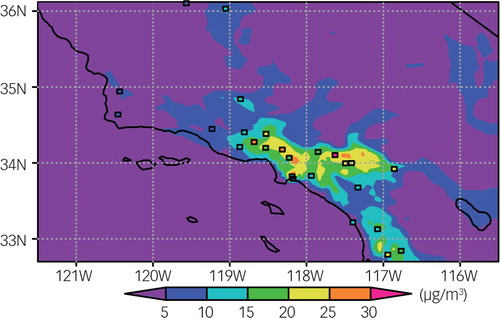
Hourly surface PM_2.5 concentrations are obtained from ARB. There are 42 surface measurement sites in Southern California (Fig. 1). The measurements were quality controlled using value-range and time-continuity checks (Jiang et al., 2013). PM_2.5 observation values less than 1 µg/m³ or exceeding 100 µg/m³ were deemed unrealistic and rejected. Time continuity was checked to eliminate singular data. Any observation y(t) will be eliminated if it does not satisfy , where denotes the previous hour and next hour, the m(t) is determined empirically. We used m(t)=10+0.5y(t) in this study.

Fig. 1 Map of the surface sites (black squares) and aircraft flight track on 2 June 2010 (coloured curve). The flight started at 01:00 PDT and ended at 07:00 PDT, lasting for 6 hours. Colours indicate the flight time.

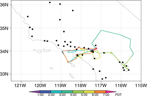
The speciated vertical profiles were assimilated from one flight made on 2 June 2010. The aircraft took off at about 01:00 local time (Pacific Daylight Time, PDT) and landed at about 07:00 PDT, corresponding universal time is from 08:00 to 14:00 UTC around Los Angeles Basin (Fig. 1). During the flight, the height of aircraft (black line) varied but was mostly between 200 and 2000 m (Fig. 2). For the planetary boundary layer (PBL) height (not shown) is mostly lower than 500 m over flight area during the night-time. The aircraft samples aerosols within and above PBL.

Fig. 2 Evolution of the flight height (black) and the total concentration of OC, NO₃, SO₄ and NH₄ (blue dashed curve) along the aircraft flight track from 01:00 to 07:00 PDT 2 June 2010.

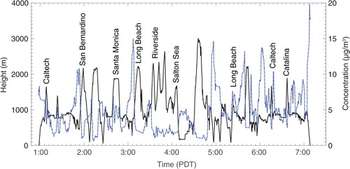
Along the flight track, speciated aerosol mass concentrations of OC, NO₃, SO₄ and NH₄ were sampled every 10 seconds. Since the measurements have much higher spatial resolution than the model has (Section 3), we thinned the measurements by averaging them for every 60 seconds. Figure 2 shows the evolution of the aerosol total concentrations along the flight track (blue dashed line). The changes of total concentration are contrary to the changes of flight height, since the aerosol concentration decreases rapidly with height.

3. Model configuration and data assimilation algorithm

We used WRF/Chem (v3.5) to simultaneously predict weather and atmospheric (chemistry) composition. The 3DVAR system utilised here is implemented following Li et al. (2013) but enhanced by a few new major features as described in this section.

3.1. WRF/Chem model configurations

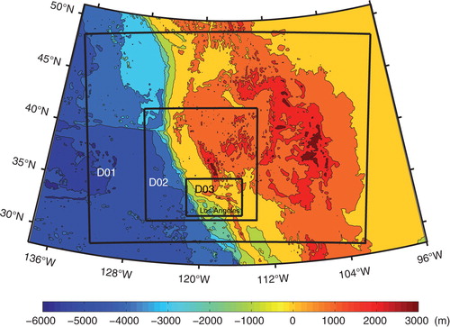
The WRF/Chem model configuration has a triple-nested domain, with a resolution of 36 km, 12 km, and 4 km, respectively (Fig. 3). The MOSAIC (Model for Simulating Aerosol Interactions and Chemistry) scheme (Zaveri et al., 2008) is selected for the representation of aerosol processes. The MOSAIC model was first implemented in the Weather Research and Forecasting (WRF) model coupled with Chemistry (WRF/Chem) by Fast et al. (2006). In the MOSAIC model, there are eight species, including elemental/black carbon (EC/BC), organic carbon (OC), nitrate (NO₃), sulphate (SO₂), chloride (Cl), ammonium (NH), sodium (Na). Other unspecified inorganic species such as silica (SiO₂), other inert minerals, and trace metals are lumped together as ‘other inorganic mass’ (OIN). A sectional approach is adopted to represent aerosol size distributions. The size bins are defined by their lower and upper dry particle diameters, and here four bins are used: 0.039–0.1 µm, 0.1–1.0 µm, 1.0–2.5 µm and 2.5–10 µm. There are thus 32 aerosol model variables in the MOSAIC model.

Fig. 3 Three-nested model domains. The innermost domain covers the Los Angeles basin, and the black square indicates the location of Los Angeles. Colours indicate topographic elevations.

The anthropogenic emissions are derived from National Emission Inventory 2005 (NEI'05) for both aerosols and trace gases (McKeen et al., 2002). The wind-driven emissions (sea salt and dust) are computed in the MOSAIC scheme and are turned on in the experiments presented later. No missions from biomass burning are included.

3.2. Data assimilation scheme

To make data assimilation computationally manageable, it is necessary to reduce the number of state/control variables. The 3DVAR used here allows combination of size bins and species to form so called lumped variables. Li et al. (2013) reduced the number of the control variables to five. Here we combine the size bins for each species in the MOSAIC scheme. The total aerosol concentrations of the eight species are the control variables in this 3DVAR system. Since the three new control variables are Cl, Na and NH₄ concentrations, the aircraft measurements of NH₄ concentrations can then be directly assimilated.

With the total concentrations of the eight species being the control variables, we have the control variable vector as , where ‘T’ stands for transpose. The incremental form of the DA system can be written as:1

Here, δx is the N-vector, known as the incremental state variable, which is defined as, δx=x−x ^b , where x ^b is the forecast or background state of the eight species that generated by the MOSAIC scheme. B is the N×N-matrix, denoting the error covariance associated with x ^b . The M-vector d=y−Hx ^b is known as the observation innovation vector, where y is an observation vector and the M×M-matrix R is the observation error covariance. H is the observation operator that computes the observation estimates from the state variables. After the increment of each state variable δx is obtained, the increment is distributed into each size, and the distribution is in proportional to the background error variance of each size bin.

With given observations, the background error covariance dictates the performance of a 3DVAR scheme to a substantial degree. We outline in brief its estimation and characteristics. To incorporate the error covariance B, it needs to be simplified. To do so, we follow the process outlined by Li et al. (2013), to factorising B into two parts:2

Here D is the standard deviation matrix and C is the correlation matrix. With this factorisation, D and c can be prescribed and calculated separately. D is a diagonal matrix whose elements are the standard deviation (SD) of all state variables in the 3D grids. D is often simplified to vary only with the vertical levels but is homogeneous in the horizontal as in Li et al. (2013).

The background error covariance B is constructed similar to that given in Li et al. (2013), but here a 3D D is used, that is, D varies vertically and is heterogeneous in the horizontal, which we use to improve the capability of the 3DVAR in representing aerosol small-scales. D is estimated using 1 month forecast differences between 24-hour and 48-hour forecasts using the well-known ‘National Meteorological Center (NMC)’ method (Parrish and Derber, 1992). The observation error is the half of D, and a vertical profile of observation errors was applied, resulted from the average of D of every level.

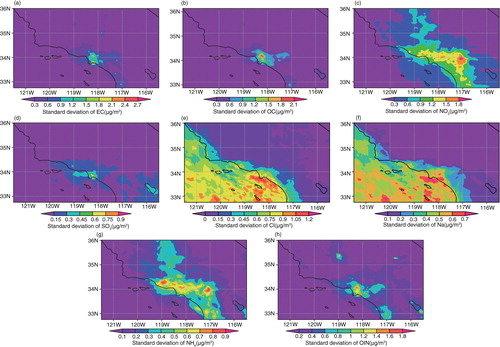
Figure 4 presents the horizontal distribution of D for all the eight species. The distributions of D are obviously different among these species. For Cl and Na, their high values of SD mainly appear over the coastal ocean and land area near the coast, since Cl and Na are primarily emitted from the ocean. High values of EC, OC and SO₄ abound near the Los Angeles downtown area due to anthropogenic emissions. Interestingly, high values of NO₃, NH₄ and OIN are spread over a wide area. The SDs for EC, OC, NO₃ and OIN are larger than other species.

Fig. 4 Surface distribution of the SD of aerosol species of EC (a), OC (b), NO₃ (c), SO₄, (d), Cl (e), Na (f), NH₄ (g) and OIN (h).

The 3D correlation matrix C can be approximately factorised three independent matrices by using Kronecker product (Li et al., 2013).3

Here, ⊗ denotes the Kronecker product, and C _x , C _y and C _z represent the correlation matrices of x, y and z directions. The horizontal correlation matrices C _x and C _y is approximately expressed using one-dimensional Gaussian function (Daley, 1991):4

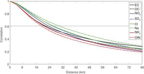
where r ₁₂ represents the correlation between two horizontal points, Δr represents the distance of these two points, and L _s represents the horizontal correlation length scale. Assuming the correlations are isotropic, the correlation scale L _s becomes the only parameter of C _x and C _y . The L _s can be estimated using the date of forecast differences from NMC method. Figure 5 shows the decrease of correlation curves with horizontal distance calculated by the forecast differences. The cross between the correlation curve and the line of (blue line) represents the length scale L _s . The L _s of Cl and Na are longer than other species, which may result from the large-scale and even distribution over the ocean. On the contrary, the shorter L _s of other species may result from the small-scale and uneven distribution.

Fig. 5 Horizontal correlation curves of the background errors for each species. The blue line denotes the length scale at the position of .

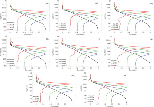
The vertical correlation matrix C _z is estimated using the NMC method (Parrish and Derber, 1992). The vertical correlation is difficultly expressed by an analytical function such as Gaussian function because of the discontinuity-like transition between the boundary layer and the free atmosphere. Figure 6 shows the vertical correlation of background errors. A common feature of the correlation between the near surface and aloft level is that the correlation reduces rapidly above 200 m. There are some differences for these species. The correlations between the surface and the height about 2000 m is about 0.2 for EC, OC, Cl and OIN, and the least is about 0.1 for NH₄.

Fig. 6 Profiles of vertical correlation of the background error for EC (a), OC (b), NO₃ (c), SO₄, (d), Cl (e), Na (f), NH₄ (g) and OIN (h). One curve represents the correlation of a given level with all the levels. The given levels include the surface and other three levels.

4. Data assimilation and forecasting experiments

Four experiments are conducted to characterise the impact of the surface and aircraft measurements on 3DVAR analyses and PM_2.5 forecasts. The first is a control experiment, which is a simulation driven by the forecast of the meteorological field without aerosol DA, often known as a free run and denoted as Control; the second a DA experiment that assimilates only the surface PM_2.5 measurements, denoted as DA-sfc; the third a DA experiment that assimilates only the aircraft profile measurements, denoted as DA-air, and the fourth a DA experiment that assimilates the surface and aircraft measurements simultaneously, denoted as DA-both. Such experiments are often referred to as OSE.

Using the model configurations described in Section 3.1, all experiments began from 02:00 PDT 2 June 2010, and then ran for 39 hours, ending at 17:00 PDT 3 June 2010. The DA experiments are applied only in the innermost domain (Fig. 3) of the model.

The observations were assimilated at 02:00 PDT 2 June 2010. While the period of the aircraft observations expands from 01:00 to 07:00 PDT 2 June 2010, only are the observations from 01:30 to 02:30 PDT (02:00 PDT±0.5 h) are assimilated. Other aircraft observations after 02:30 PDT are used to evaluate the subsequent forecasts. The surface observations are hourly PM_2.5. The 3DVAR analysis fields are used to initialise the aerosol variables in the WRF/Chem model at 02:00 PDT 2 June 2010. The meteorological fields are initialised using the North American Regional Reanalysis (NARR) (Mesinger et al., 2006).

5. Results and analyses

This section presents the results obtained from the four experiments. The 3DVAR analyses and subsequent forecasts are evaluated using the surface PM_2.5 and aircraft speciated profile observations, respectively.

5.1. Background, innovation and analysis increment

Figure 7 depicts the background, overlaid with surface observations of PM_2.5 at 02:00 PDT 2 June 2010. The background shows two areas with high concentration near Los Angeles (118.11W, 34.02N) and Fontana (117.50W 34.10N). The observed and background PM_2.5 concentrations are comparable both on these two areas and most of the other areas, but significant differences are seen at some stations. For example, the observed concentration at Los Angeles and Long Beach (118.11W, 33.80N) is remarkably lower than that of the background, and thus the innovations should be negative values (the observation minus the background).

Fig. 7 Background (shaded) and surface observations (squares) of PM_2.5 at 02:00 PDT 2 June 2010. The colour differences between the shaded areas and squares indicate the innovations of the surface PM_2.5 concentration observations.

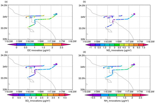
Figure 8 shows the innovations of the aircraft observations of four species (OC, NO₃, SO₄ and NH₄). The background field is from the initialisation time and the aircraft observations are from 01:30 to 02:30 PDT, 2 June 2010. In Fig. 8, the values are mostly positive, indicating that the observed concentrations are higher than that of the background and thus the background under-predicts the concentration.

Fig. 8 Observation innovations of species of OC (a), NO₃ (b), SO₄ (c), and NH₄ (d) along the aircraft flight track between 01:30 and 02:30 PDT 2 June 2010.

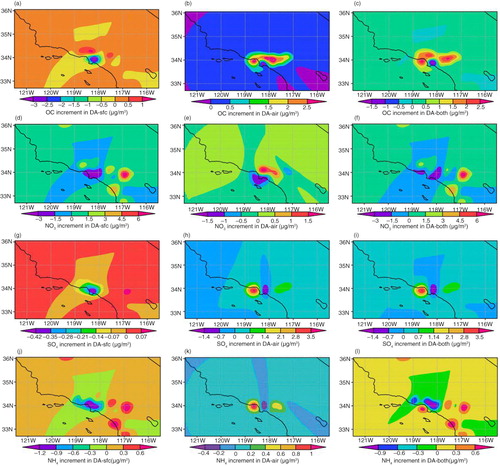
Figure 9 shows the analysis increments of four control variables (OC, NO₃, SO₄ and NH₄) from three DA experiments. For the DA-sfc experiment, the increments of the four species display similar spatial distributions. The magnitudes of the increments are different. The large negative increment of NO₃ is coincident with the distribution of innovation (Fig. 8b) and the magnitude of the SD (Fig. 4c). For the DA-air experiment (Fig. 9), the increments do not display similar spatial distributions for different species.

Fig. 9 Surface distributions of increments of the species in three DA experiments. Each column contains the increments from the same DA experiment. Figures in the left, middle and right columns are from DA-sfc, DA-air and DA-both, respectively. Figures in each row are from the species of OC (a, b, and c), NO₃ (d, e and f), SO₄ (g, h and i) and NH₄ (j, k and l) from top to bottom, respectively.

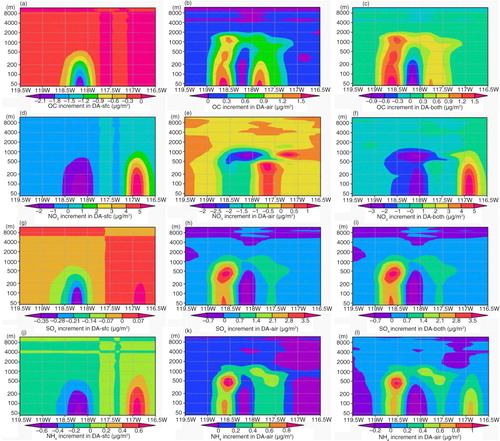
Figure 10 shows the vertical section of the increments of OC, NO₃, SO₄, NH₄ and PM_2.5 along 33.80N. In the DA-sfc experiment, the increments spread upward from the surface. The locations of the major surface increments are consistent with the horizontal increments (Fig. 9). In the DA-air experiment, the increments come from the aircraft profile observation. Note that some increments near the surface are larger than that on the level of aircraft (Fig. 10b). This is because the vertical correlation between the surface and aircraft level is significant, which results in the increment spread from the aircraft level to the surface. And the SD on the surface is larger than that on the aircraft level, which can enhance the increment on the surface. In contrast, as the SD decreases rapidly above the height of the boundary layer, the increments commonly decrease with height on upper levels. For all of species, it seems that the pattern of the increment with DA-both is more like the pattern with DA-air, since the less observation error of aircraft data, and the aircraft observation is denser than the surface observation.

Fig. 10 Same as Fig. 9 except for vertical sections along 33.80N.

5.2. Data assimilation analysis

To characterise the data assimilation analyses, we compare the results of the four experiments against the observations that are assimilated, which is known as ‘sanity check’. Three basic statistical measures, mean bias (BIAS), root-mean-square error (RMSE), and correlation coefficient (CORR), are utilised for the evaluations.

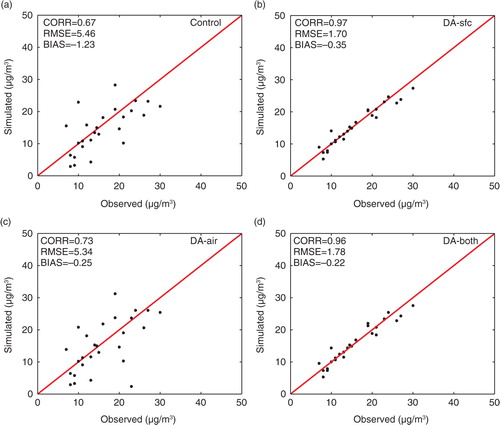
Figure 11 shows the scatter plots of the model versus the observed surface PM_2.5 mass concentrations at 02:00 PDT, 2 June 2010, the time when the model was initialised. Compared with the control experiment, all the three DA experiments are closer to the observed PM_2.5. The CORR in the DA-sfc experiment (Fig. 11b) increased by 0.30, and the RMSE and the absolute BIAS decreased by more than 60%. The DA-air experiment (Fig. 11c) also shows an improvement, compared to the control experiment. Note that these evaluations are based on the surface observations, and the aircraft observations are independent from the surface observation. The result indicates that the aircraft observations are accordant with the surface observations, though they are not in the same levels. Also, the improvement of DA-air is mainly around the area of Los Angeles (Fig. 6), there is little influence on the other areas far away the area of aircraft observations. The absolute BIAS of the DA-both experiment (Fig. 11d) is the smallest among all the experiments, while the RMSE and CORR are comparable with that of the DA-sfc.

Fig. 11 Scatter plots of observed concentrations of PM_2.5 versus simulated concentrations of PM_2.5 from the experiments of Control (a), DA-sfc (b), DA-air (c) and DA-both (d) surface over 02:00 PDT initialisations. The observed concentrations of PM_2.5 are from the 42 surface stations, and they are used in the assimilation of DA-sfc and DA-both.

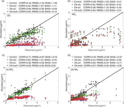
Figure 12 shows the scatter plots of the 3DVAR analysis versus the aircraft observations. With DA-sfc, the improvement is limited. The evaluations of DA-air and DA-both are generally higher than that of Control except for NO₃. Both the DA-air and DA-both experiments show a marginal improvement, compared to the control experiment; however, the improvement is limited in areas with high concentration. For example, the large values of the observed concentration are nearly 5.0 µg/m³, but that of the simulated concentration are no more than 3.0 µg/m³ in all the data assimilation experiments (Fig. 12b). Since the number of observations with larger values is small, and they are surrounded by a large number of observations with low values, the large number of observations determines the size of increments.

Fig. 12 Scatter plots of observed concentrations of OC (a), NO₃ (b), SO₄ (c) and NH₄ (d) versus simulated concentrations during 01:30 to 02:30 PDT initialisations. The CORR, RMSE and BIAS are estimated for all the four experiments: Control (red start), DA-sfc (blue dot), DA-air (green dot) and DA-both (black dot). The observed concentrations of species are from the aircraft observations, and they are used in the assimilation of DA-air and DA-both.

5.3. Evaluation of forecasts

The forecasts are evaluated using the hourly surface PM_2.5 observations taken during the forecasting period from 02:00 PDT 2 June to 17:00 PDT 3 June 2010. Using aircraft observations, the speciated forecasts from 2:30 to 07:00 PDT, 2 June 2010 are evaluated. Since the aircraft observations are continuous, their hourly mean is compared with data from the hourly forecasting.

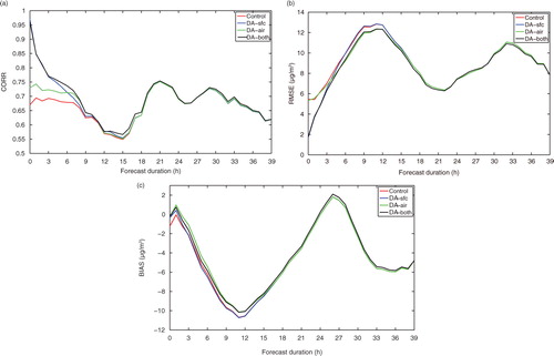
Figure 13 shows the CORR and RMSE of the PM_2.5 forecasts against the surface observations as a function of forecasting duration. In Fig. 13a, the CORR of the three DA forecasts are higher than that of the Control forecast during the earlier forecasts. The CORR of the DA-both is very similar with that of the DA-sfc during the first 4 hours. For the forecast between 4 and 18 hours, the CORR is persistently higher with DA-both than with DA-sfc. In Fig. 13b and 13c, the RMSE and BIAS of the DA-both experiment is persistently lower during the first 15 hours than that of the other experiments. Interestingly, the first 3-hour forecast is more skilful with DA-sfc than DA-air in terms of both CORR and RMSE. Between 4 and 15 hours, the forecast is more skilful with DA-air than DA-sfc. It suggests that the assimilation of aircraft observations can result in positive and more persistent effect on surface PM_2.5 forecast.

Fig. 13 Correlations (CORR) (a), root-mean-square errors (RMSE) (b) and BIAS (c) of the total PM_2.5 concentration forecasts against observations as a function of forecast duration. All of them are calculated against the observations from 42 surface stations during the period from 02:00 PDT 2 June to 17:00 PDT 3 June 2010.

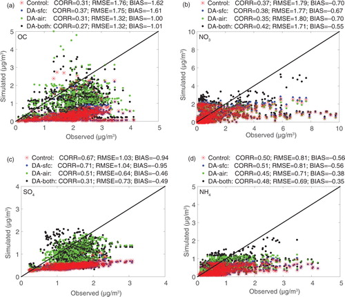
Figure 14 shows the scatter plots of the model concentrations versus aircraft concentrations of species during 02:30–07:00 PDT. Both RMSE and absolute BIAS are reduced in the DA-air and DA-both experiments compared to the control experiment. Thus, the assimilation of aircraft observations exhibits a positive impact on the forecast skill of different species. However, the reductions drop quickly by 5 hours (from 09:00 to 14:00) after the initialisation, suggesting that the improvements of the assimilation experiments decrease rapidly. The reason could be that the assimilated aircraft observations are localised within a limited area.

Fig. 14 Same as Fig. 12 except for the observed concentrations versus forecast concentrations during 02:30–07:00 PDT 2 June.

6. Summary and conclusions

During the CalNex campaign a variety of aerosol observations were acquired from aircraft, ship, and ground-based platforms. Using a 3DVAR system, the aircraft speciated 3D profiles and surface PM_2.5 from ARB are assimilated. We have carried out OSEs to illustrate impacts of vertical profiles and surface observations on the analysis fields and subsequent forecasts.

The 3DVAR system was implemented following the formulation given in Li et al. (2013). To assimilate different types of speciated measurements simultaneously and effectively, we enhanced the 3DVAR system by using all eight species represented in the MOSAIC scheme as control variables, and further by incorporating horizontally inhomogeneous background error SD. This enhanced 3DVAR system was then used to assimilate speciated surface observations and 3D aircraft profiles during CalNex. We performed three DA experiments, assimilating solely the surface observations (DA-sfc), solely the aircraft 3D profiles (DA-air), and both (DA-both). These DA experiments began at 02:00 PDT 2 June 2010, assimilating surface observations at 02:00 PDT and aircraft observations from 01:30 to 02:30 PDT. As a reference, one control experiment without DA (Control) was also performed. From these experiments, the impact of the surface observations and profiles on forecast skills was analysed.

The comparison to the hourly surface PM_2.5 observations shows that the forecast skill of the DA-both experiment is the highest among the three experiments (Figs. 11 and 13). The forecast skill improvement is persistent, at least, out to 15 hours. In the DA-sfc experiment, the forecast skill improvement is seen mostly during the first few hours and only out to 10 hours. In contrast, the impact of the aircraft observations persists longer in time and at least out to 15 hours as in the DA-sfc experiment. When evaluating the experiments against the aircraft speciated concentration profiles, the skills of the DA-air and DA-both tends to be higher than that of the Control. In contrast, the forecast skill of the DA-sfc shows no appreciable improvements over the Control.

The results from the experiments suggest that the aircraft vertical profiles observations, although localised within a limited area, contribute more to forecast skill improvement, supporting a hypothesis that vertical profiles are more effective in extending forecast skills. Such results might be the consequence of ineffectiveness of the propagation of the information of surface measurements from the surface to the upper air in the DA scheme. It is known that the vertical correlation in the background error covariance is the primary mechanism of vertical propagation in a 3DVAR system. The vertical correlation is more complex for aerosol variables than that for the meteorology variable (Saide et al., 2013). This ineffectiveness may be related to the disagreement between the background error vertical correlation and the actual boundary layer structure. The vertical correlation of the background error covariance is fixed with an average value, but the actual boundary layer structure varies with spatio-temporal distribution. In the model domain, the inland boundary layer is commonly higher than the one seen over the ocean (Li et al., 2013). Thus, the background error vertical correlation of inland areas may be overestimated.

We note that, due to the short time of availability of vertical profile measurements, the results are based on DA experiments performed at one single time. This is thus a case study. The results are more suggestive than conclusive. An extended period of time or experiments with other field campaigns are needed to confirm the results presented here.

7. Acknowledgements

This research was supported by the National Natural Science Foundation of China (41275128 and 41206163). We gratefully thank the California Air Resources Board (www.arb.ca.gov/homepage.htm) and NOAA Earth System Research Laboratory Chemical Sciences Division (www.esrl.noaa.gov/csd/groups/csd7/measurements/2010calnex), for providing the download of aerosol surface and aircraft observations.

References

- Benedetti A. , Morcrette J.-J. , Boucher O. , Dethof A. , Engelen R. J. , co-authors . Aerosol analysis and forecast in the European Centre for Medium-Range Weather Forecasts Integrated Forecast System: 2. Data assimilation. J. Geophys. Res. 2009; 114: 13205.
- Bocquet M. , Elbern H. , Eskes H. , Hirtl M. , Zabkar R. , co-authors . Data assimilation in atmospheric chemistry models: current status and future prospects for coupled chemistry meteorology models. Atmos. Chem. Phys. 2015; 15: 5325–5358.
- Daley R . Atmospheric data analysis (Cambridge Atmospheric and Space Science Series). 1991; Cambridge, UK: Cambridge University Press.
- Denby B. , Schaap M. , Segers A. , Builtjes P. , Horálek J . Comparison of two data assimilation methods for assessing PM10 exceedances on the European scale. Atmos. Environ. 2008; 42: 7122–7134.
- Diner D. J. , Ackerman T. P. , Anderson T. L. , Bosenberg J. , Braverman A. J. , co-authors . PARAGON: an integrated approach for characterising aerosol climate impacts and environmental interactions. B. Am. Meteorol. Soc. 2004; 85: 1491–1501.
- Fast J. D. , Gustafson W. I. Jr. , Easter R. C. , Zaveri R. A. , Barnard J. C. , co-authors . Evolution of ozone, particulates, and aerosol direct radiative forcing in the vicinity of Houston using a fully coupled meteorology-chemistry-aerosol model. J. Geophys. Res. 2006; 111: 21305.
- Jiang Z. , Liu Z. , Wang T. , Schwartz C. S. , Lin H.-C. , co-authors . Probing into the impact of 3DVAR assimilation of surface PM10 observations over China using process analysis. J. Geophys. Res. Atmos. 2013; 118: 6738–6749.
- Kalnay E . Lahoz W. A. , Khattatov B. , Ménard R . Ensemble Kalman filter: current status and potential. Data Assimilation: Making Sense of Observations. 2010. Springer, Berlin, pp. 69–92.
- Lee H. J. , Liu Y. , Coull B. A. , Schwartz J. , Koutrakis P . A novel calibration approach of MODIS AOD data to predict PM2.5 concentrations. Atmos. Chem. Phys. 2011; 11: 7991–8002.
- Levy R. C. , Remer L. A. , Kleidman R. G. , Mattoo S. , Ichoku C. , co-authors . Global evaluation of the collection 5 MODIS dark-target aerosol products over land. Atmos. Chem. Phys. 2010; 10: 10399–10420.
- Li Z. , Zang Z. , Li Q. B. , Chao Y. , Chen D. , co-authors . A three-dimensional variational data assimilation system for multiple aerosol species with WRF/Chem and an application to PM2.5 prediction. Atmos. Chem. Phys. 2013; 13: 4265–4278.
- Liu Z. , Liu Q. , Lin H.-C. , Schwartz C. S. , Lee Y.-H. , co-authors . Three-dimensional variational assimilation of MODIS aerosol optical depth: implementation and application to a dust storm over East Asia. J. Geophys. Res. 2011; 116: 23206.
- Mangold A. , De Backer H. , De Paepe B. , Dewitte S. , Chiapello I. , co-authors . Aerosol analysis and forecast in the European Centre for Medium-Range Weather Forecasts Integrated Forecast System: 3. Evaluation by means of case studies. J. Geophys. Res. 2011; 116: 03302.
- McKeen S. A. , Wotawa G. , Parrish D. D. , Holloway J. S. , Buhr M. P. , co-authors . Ozone production from Canadian wildfires during June and July of 1995. J. Geophys. Res. 2002; 107: 4192.
- Mesinger F. , DiMego G. , Kalnay E. , Shafran P. , Ebisuzaki W. , co-authors . North American regional reanalysis. B. Am. Meteorol. Soc. 2006; 87: 343–360.
- Morgan W. T. , Allan J. D. , Bower K. N. , Capes G. , Crosier J. , co-authors . Vertical distribution of submicron aerosol chemical composition from North-Western Europe and the North-East Atlantic. Atmos. Chem. Phys. 2009; 9(15): 5389–5401.
- Pagowski M. , Grell G. A. , McKeen S. A. , Peckham S. E. , Devenyi D . Three-dimensional variational data assimilation of ozone and fine particulate matter observations: some results using the weather research and forecasting-chemistry model and grid-point statistical interpolation. Q. J. Roy. Meteorol. Soc. 2010; 136: 2013–2024.
- Parrish D. F. , Derber J. C . The national meteorological center spectral statistical interpolation analysis. Mon. Weather Rev. 1992; 120: 1747–1763.
- Saide P. E. , Carmichael G. R. , Liu Z. , Schwartz C. S. , Lin H.-C. , co-authors . Aerosol optical depth assimilation for a size-resolved sectional model: impacts of observationally constrained, multiwavelength and fine mode retrievals on regional scale forecasts. Atmos. Chem. Phys. 2013; 13: 10425–10444.
- Schwartz C. S. , Liu Z. , Lin H.-C. , McKeen S. A . Simultaneous three-dimensional variational assimilation of surface fine particulate matter and MODIS aerosol optical depth. J. Geophys. Res. 2012; 117: D13202.
- Tombette M. , Mallet V. , Sportisse B . PM10 data assimilation over Europe with the optimal interpolation method. Atmos. Chem. Phys. 2009; 9: 57–70.
- van Donkelaar A. , Martin R. V. , Brauer M. , Kahn R. , Levy R. , co-authors . Global estimates of ambient fine particulate matter concentrations from satellite-based aerosol optical depth: development and application. Environ. Health Persp. 2010; 118: 847–855.
- Wang Y. , Sartelet K. N. , Bocquet M. , Chazette P . Assimilation of ground versus lidar observations for PM10 forecasting. Atmos. Chem. Phys. 2013; 13: 269–283.
- Wang Y. , Sartelet K. N. , Bocquet M. , Chazette P . Modelling and assimilation of lidar signals over Greater Paris during the MEGAPOLI summer campaign. Atmos. Chem. Phys. 2014; 14: 3511–3532.
- Weber R. , Orsini D. , Duan Y. , Baumann K. , Kiang C. S. , co-authors . Intercomparison of near real time monitors of PM2.5 nitrate and sulfate at the U.S. Environmental Protection Agency Atlanta Supersite. J. Geophys. Res. 2003; 108(D7): 8421–8435.
- Zaveri R. A. , Easter R. C. , Fast J. D. , Peters L. K . Model for Simulating Aerosol Interactions and Chemistry (MOSAIC). J. Geophys. Res. 2008; 113: D13204.
- Zhang J. , Reid J. S. , Westphal D. , Baker N. , Hyer E . A system for operational aerosol optical depth data assimilation over global oceans. J. Geophys. Res. 2008; 113: D10208.