Ship-based observations of atmospheric potential oxygen and regional air–sea O₂ flux in the northern North Pacific and the Arctic Ocean

Abstract

Simultaneous observations of atmospheric potential oxygen (APO=O₂+1.1×CO₂) and air–sea O₂ flux, derived from dissolved oxygen in surface seawater, were carried out onboard the research vessel MIRAI in the northern North Pacific and the Arctic Ocean in the autumns of 2012–2014. A simulation of the APO was also carried out using a three-dimensional atmospheric transport model that incorporated a monthly air–sea O₂ flux climatology. By comparing the observed and simulated APO, as well as the observed and climatological air–sea O₂ fluxes, it was found that the large day-to-day variation in the observed APO can be attributed to the day-to-day variation in the local air–sea O₂ fluxes around the observation sites. It was also found that the average value of the observed air–sea O₂ fluxes was systematically higher than that of the climatological O₂ flux. This could explain the discrepancy between the observed and simulated seasonal APO cycles widely seen at various northern hemispheric observational sites in the fall season.

• atmospheric potential oxygen
• air-sea O₂ flux
• ship observation

1. Introduction

High precision measurements of the atmospheric O₂/N₂ ratio have been carried out since the early 1990s to estimate the global terrestrial biospheric and oceanic CO₂ uptake (e.g. Keeling et al., 1996; Bender et al., 2005; Manning and Keeling, 2006; Tohjima et al., 2008; Ishidoya et al., 2012a, 2012b). The approach is based on the global mean O₂:CO₂ exchange ratios for the terrestrial biospheric O₂ and CO₂ fluxes (−1.1) and fossil fuel combustion (−1.17, −1.44 and −1.95 for coal, liquid and gaseous fuels, respectively) (Keeling, 1988; Severinghaus, 1995). By using the O₂:CO₂ exchange ratio of −1.1 for terrestrial biospheric activities, a quantity known as atmospheric potential oxygen (APO) is defined by APO=O₂+1.1×CO₂ (Stephens et al., 1998). Since APO is essentially conserved for terrestrial biospheric activities, it has been used to evaluate air–sea O₂ fluxes associated with marine biological and physical processes (e.g. Keeling et al., 1998; Garcia and Keeling, 2001; Nevison et al., 2012).

In order to increase our understanding of the relationship between the local air–sea O₂ flux variation and APO, we need to observe APO just above the sea surface. However, shipboard observations of APO are still limited (Stephens et al., 2003; Tohjima et al., 2005, 2012, 2015; Battle et al., 2006; Thompson et al., 2007, 2008). Stephens et al. (2003) carried out continuous measurements of the atmospheric O₂/N₂ ratio and CO₂ concentration in the equatorial Pacific during April and May 1998 and in the Southern Ocean during October 1998. Thompson et al. (2008) also measured the atmospheric O₂/N₂ ratio and CO₂ concentration continuously in the southern Pacific Ocean during February 2003 and April 2004. Both of these studies revealed larger spatiotemporal variations in the O₂/N₂ ratio than those in CO₂. As explained in these papers, the difference arises from the fact that the equilibration time for O₂ between the atmosphere and the surface ocean is much shorter than that for CO₂ since the air–sea exchange of CO₂ between the atmosphere and the ocean is influenced by an additional process involving the carbonate dissociation effect (Keeling et al., 1993). Therefore, short-term variations in APO can be exploited to evaluate local air–sea O₂ fluxes due to marine biological activities and thermally induced solubility changes.

Thompson et al. (2008) also compared the observed APO with those simulated using an atmospheric transport model (Heimann and Körner, 2003) driven by air–sea O₂ and CO₂ fluxes estimated from an ocean biogeochemistry model (Buitenhuis et al., 2005) or from climatologies (Najjar and Keeling, 2000; Takahashi et al., 2002). They found that the simulated APO agreed qualitatively with the observed characteristics of the APO latitudinal variation but underestimated the magnitude of the observed APO maximum in the mid-southern latitudes. On the other hand, Tohjima et al. (2005, 2012, 2015) have carried out long-term observations of APO in the Pacific region since the early 2000, elucidating in much more detail the salient features of the seasonal cycle, latitudinal gradient and secular trend in APO. In one of their studies (Tohjima et al., 2012), the observed seasonal APO cycles were reproduced relatively well by an atmospheric transport model (Maksyutov and Inoue, 2000) driven by an air–sea climatology of O₂ and N₂ fluxes (Garcia and Keeling, 2001).

In order to advance our understanding of the contribution the local air–sea O₂ fluxes make to the observed variations in APO, as well as to validate the air–sea O₂ flux climatologies reported in past studies (e.g. Garcia and Keeling, 2001), simultaneous observations of APO and the air–sea O₂ flux are needed. To achieve this objective, we collected flask air samples onboard the research vessel MIRAI during its cruises in the northern North Pacific and the Arctic Ocean during the fall seasons of 2012–2014, to analyse for the atmospheric O₂/N₂ ratio, CO₂ concentration and stable isotopic ratio (δ¹³C) of CO₂, along with continuous measurements of dissolved oxygen in the surface seawater. Here δ¹³C of CO₂ measurements allow us to separate the atmosphere–terrestrial biosphere CO₂ exchange from the one between the atmosphere and the ocean (e.g. Keeling et al., 1989; Nakazawa et al., 1993; Battle et al., 2000). The terrestrial biosphere preferentially uptakes CO₂ with a lower δ¹³C value, enriching δ¹³C of CO₂ left behind in the atmosphere. On the other hand, a change in the atmospheric δ¹³C of CO₂ due to an exchange of 1 mol of CO₂ between the atmosphere and the ocean is about 10 % of that observed between the atmosphere and the terrestrial biosphere. Therefore, simultaneous observations of APO and δ¹³C of CO₂ can enhance our understanding of the causes of variations in the observed APO, since APO variations mainly reflect air–sea gas exchanges.

In this paper, we present observational results of these measurements and discuss the possible relationship between the observed APO and the air–sea O₂ fluxes derived from the observed dissolved oxygen concentration. We also compare the observed APO with simulated APO using an atmospheric transport model (Taguchi et al., 2002) driven by climatological air–sea O₂ and N₂ fluxes (Garcia and Keeling, 2001), to evaluate differences between the observed and climatological O₂ fluxes during the fall season in the northern North Pacific and the Arctic Ocean.

2. Method

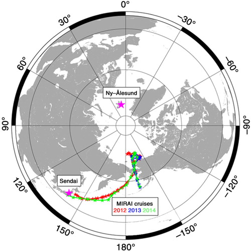
Air samples to measure the O₂/N₂ ratio, CO₂ concentration and δ¹³C of CO₂ were collected on average once per day onboard the research vessel MIRAI for the period 5 September–15 October 2012, 29 August–6 October 2013, and 1 September–9 October 2014. The MIRAI cruise reports are available from the Japan Agency for Marine–Earth Science and Technology database (www.godac.jamstec.go.jp/catalog/doc_catalog/e/index.html). Locations where the air samples were collected are shown in Fig. 1. Each air sample was taken from an air intake at a flow rate of 7 L·min⁻¹ using a piston pump (GAST co., LOA) and filled into a 1 L stainless-steel flask after removing water vapour using a cold trap at −80 °C. During the air sampling, an inner pressure of the flask was kept at an absolute pressure of 0.55 MPa using a backpressure valve (Tohjima et al., 2003). The air intake was mounted at a height of 25 m a.s.l. on the foredeck. The 1-L stainless-steel flasks used in 2012 were each equipped with a metal-seal valve (Nupro co., SS-4H) on each side. However, we found that a mass-dependent fractionation of O₂ and N₂ due to a small leak through the valve (e.g. Langenfelds et al., 1999) was significant for some flasks. The significance of the fractionation was confirmed by the simultaneously measured values of the Ar/N₂ ratio, stable isotopic ratios of N₂, O₂ and Ar. Therefore, for the 2013 and 2014 cruises, we used flasks equipped with two metal-seal valves on each side to equalise the inner pressure of the flask to the pressure between the two metal-seal valves. With this improvement, the mass-dependent fractionation was reduced significantly.

Fig. 1 Locations where air samples were collected (small stars) onboard MIRAI for the period 5 September–15 October 2012 (red) 29 August–6 October 2013 (blue), and 1 September–9 October 2014 (green). Locations of Ny-Ålesund Station, Svalbard, Norway, and Sendai, Japan, are also shown (large purple stars).

The O₂/N₂ and Ar/N₂ ratios, as well as stable isotopic ratios of N₂, O₂ and Ar, were measured using a mass spectrometer (Thermo Scientific Delta-V) at the National Institute of Advanced Industrial Science and Technology (AIST) (Ishidoya and Murayama, 2014). The CO₂ concentration and δ¹³C of CO₂ were measured using a non-dispersive infrared analyzer (Li-7000) and a mass spectrometer (Thermo Electron Delta-S), respectively, at Tohoku University (Tanaka et al., 1983; Nakazawa et al., 1997). The O₂/N₂ ratio and δ¹³C of CO₂ are reported in:1 2

where subscripts ‘sa’ and ‘st’ indicate the sample air and the standard air, respectively. An increase of one mole of O₂ in 10⁶ moles of air corresponds to a 4.8 per meg change in δ(O₂/N₂) since O₂ is 20.95 % of dry air (Machta and Hughes, 1970). In this study, measured values of δ(O₂/N₂) in each air sample were determined against our primary standard air (cylinder No. CRC00045) with a reproducibility of ±3 per meg. The CO₂ concentration was determined against our air-based CO₂ standard gas system with a precision of better than ±0.05 ppm (Tanaka et al., 1983), and δ¹³C of CO₂ was determined against a primary standard CO₂ produced by reacting NBS-18 with 100 % phosphoric acid at 25 °C with a precision of 0.02 ‰ (Nakazawa et al., 1997). In this study, measured δ(O₂/N₂) values were corrected for the mass-dependent fractionation of O₂ and N₂by subtracting simultaneously measured Δδ(Ar/N₂)/3 from the measured δ(O₂/N₂) assuming that the variations in the atmospheric δ(Ar/N₂) during the period of respective cruises were very small (e.g. Cassar et al., 2008) [δ(Ar/N₂) is defined in the same way as δ(O₂/N₂) but for ⁴⁰Ar/¹⁴N¹⁴N ratio]. Here Δ denotes the difference between the measured δ(Ar/N₂) values and the average of the measured values of δ(Ar/N₂) for the corresponding cruises. A typical correction was 3.0 per meg for a flask equipped with two metal-seal valves on each side, which was less than 50 % of the correction needed for a flask equipped with one metal-seal valve on each side (6.6 per meg). By using the measured CO₂ concentration and the corrected δ(O₂/N₂), APO is calculated as:3

where [CO₂] is the CO₂ concentration in ppm, −1.1 is the O₂:CO₂ exchange ratio for the terrestrial biospheric activity, X_O2 =0.2095 is the mole fraction of atmospheric O₂ (Machta and Hughes, 1970) and 381 is an arbitrary reference. It is noted that many previous APO studies expressed the measured values on the Scripps Institution of Oceanography (SIO) scale (e.g. Manning and Keeling, 2006; Kozlova et al., 2008; van der Laan et al., 2014) although the scale is not traceable to the International System of Units. A detailed comparison between our O₂/N₂ scale and the SIO scale is needed some time in the near future. If we simply compare our APO values obtained north of 55 °N (70 °N on average) with the average APO observed (based on the SIO scale) at Alert (82 °N, 63 °W), Canada and at Cold Bay (55 °N, 163 °W), Alaska during the same time period (Keeling et al., 1998; Keeling and Manning, 2014) (the APO data observed by SIO are taken from the Scripps O₂ Program database; www.scrippso2.ucsd.edu), then the APO values reported in this study are higher by about 370 per meg on average.

To compare the observed APO with those simulated using climatological air–sea O₂ and N₂ fluxes, we used a three-dimensional atmospheric transport model developed at the National Institute of Advanced Industrial Sciences and Technology, Tsukuba, Japan (Taguchi, 1996; Taguchi et al., 2002) (hereafter referred to as STAG). The STAG model is based on the NIRE-CTM 96 model and has a horizontal resolution of 1.125 ° and 60 vertical levels; advection is calculated using a semi-Lagrangian scheme. In this study, model simulations were performed using the European Centre for Medium-Range Weather Forecasts reanalysed meteorological data (ERA-Interim). Monthly seasonal climatological values of the air–sea O₂ and N₂ fluxes (hereafter referred to as F_{O2_cli} and F_{N2_cli} , respectively) were taken from the TransCom experimental protocol (Garcia and Keeling, 2001; Blaine, 2005). The climatology of O₂ flux is based on weighted linear least squares regressions using monthly heat flux anomalies for spatial and temporal interpolation of historical O₂ data; the climatology of N₂ flux is computed as the product of the heat flux anomaly times the temperature derivative of the N₂ solubility (Garcia and Keeling, 2001). Model-based APO was calculated according to:4

Here, [O₂] and [N₂] are the simulated respective concentrations of O₂ and N₂ in ppm of dry air, and X_N2 =0.7808 is the fraction of N₂ in the atmosphere. It should be noted that APO is not only driven by air–sea O₂ and N₂ fluxes but also by air–sea CO₂ flux, although it is clear that the air–sea O₂ and N₂ fluxes account for much of the variations in APO on synoptic-to-seasonal time scales, due to the dampening of CO₂ flux by the ocean carbonate chemistry. Nevertheless, to examine the contribution of air–sea CO₂ flux on APO (APO_{CO2_oc} ) more quantitatively, we also calculated the CO₂ concentration using the STAG model that incorporated the monthly climatological air–sea CO₂ flux (Takahashi et al., 2009), and converted it to APO in per meg as:5

Here, [CO_{2_oc}] is the simulated CO₂ concentration, driven by the air–sea CO₂ flux, in ppm of dry air. We used detrended values of APO_{CO2_oc} in this study, and discuss its contributions to the day-to-day and seasonal variations in APO below. Detailed evaluations of the effect of air–sea CO₂ flux on APO are also found in Rödenbeck et al. (2008) and Tohjima et al. (2012).

In this study, we also made continuous measurements of dissolved oxygen at a water depth of 5 m at 1-minute intervals. For the measurements, an optical oxygen sensor (RINKO-II, JFE Advantech Co., Ltd., Kobe, Japan) was used, along with a thermosalinograph (SBE 45, Sea-Bird Electronics, Inc., Bellevue, Washington, USA). The optical oxygen sensor was characterised with standard gases by means of a nonlinear calibration equation (Uchida et al., 2010) with slight modification before each cruise. Raw data from the optical oxygen sensor and temperature and salinity data from the thermosalinograph were used to calculate dissolved oxygen. The dissolved oxygen data were determined as an output from the linear regression as a function of uncorrected dissolved oxygen (obtained from the Winkler method) (Dickson, 1996), sea water temperature and time. A bias in the Winkler method due to iodate interference was corrected by subtracting 0.52 µmol·kg⁻¹ from the dissolved oxygen data (Wong and Li, 2009). Precisions of the dissolved oxygen measurements were estimated to be 2 µmol·kg⁻¹ for the samples in 2012 and 1 µmol·kg⁻¹ for the samples in 2013 and 2014. Details of the dissolved oxygen measurement system on MIRAI are given in Uchida et al. (2015). The observed dissolved oxygen was used to calculate air–sea O₂ flux as:6

Here, F_{O2_obs} (µmol·m⁻²·s⁻¹) is the air–sea O₂ flux (positive value denotes flux emitted from the ocean to the atmosphere), K_O2 (m·s⁻¹) is the gas exchange velocity for O₂ (Wanninkhof, 1992) and ρ (kg·m⁻³) is the density of seawater. [O₂] and [O₂]_sat denote the observed and saturated concentrations of dissolved oxygen (µmol·kg⁻¹), respectively. K_O2 is empirically expressed as:7

where8

Here u is the wind speed at height 10 m a.s.l., Sc_O2 is the Schmidt number for oxygen, t is the sea surface temperature (SST) in degree Celsius. [O₂]_sat is defined by:9 10 11 12

Here (µmol·kg⁻¹) is the solubility of O₂ calculated from eq. (8) in Garcia and Gordon (1992), P is the sea level atmospheric pressure (atm) and the coefficients A₀, A₁, A₂, A₃, A₄, A₅, B₀, B₁, B₂, B₃ and C₀ are taken from Benson and Krause (1984) (also listed in Table 1 in Garcia and Gordon, 1992). T_s is the scale temperature defined in Garcia and Gordon (1992). p_sw (atm) is the vapour pressure of water from eq. (10) in Weiss and Price (1980), T (K) and S are the absolute temperature of SST and the Practical Salinity, respectively. [O₂], and p_sw values are also related to oxygen partial pressure in surface seawater, (atm), as:13

We will use the obtained F_{O2_obs} and values to interpret variations in the APO observed during the MIRAI cruises. It should be noted that we neglected the bubble effects on F_{O2_obs} , which is caused by steady state O₂ anomaly required to balance O₂ injected below the surface by bubbles (Keeling et al., 1993, 1998). Keeling et al. (1998) noted that the bubble effects would account for at most 20 % of the ‘[O₂]–[O₂]_sat’ values in eq. (6). Therefore, the F_{O2_obs} values in this study could be overestimated by at most 20 % relative to the actual air–sea O₂ flux.

3. Results and discussion

3.1. δ(O₂/N₂), CO₂ concentration and δ ¹³C of CO₂ observed onboard a research vessel MIRAI

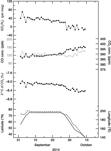
Figures 2–4 show the temporal variations in δ(O₂/N₂), CO₂ concentration and δ¹³C of CO₂ observed onboard MIRAI for the period 5 September–15 October 2012, 29 August–6 October 2013, and 1 September–9 October 2014, respectively. Sampling locations (in latitude and longitude) are also shown at the bottom of each graph. As seen in Figs. 2–4, δ(O₂/N₂) and δ¹³C show a gradual decrease with time, while CO₂ shows a gradual increase. Negative correlations of δ(O₂/N₂) and δ¹³C with CO₂ were also observed in the day-to-day variations. It is known that δ(O₂/N₂) and δ¹³C are negatively correlated with CO₂ due to fossil fuel combustion and terrestrial biospheric processes (e.g. Keeling et al., 1993; Nakazawa et al., 1997). Furthermore, while seasonal and subseasonal variations in δ(O₂/N₂) are also affected significantly by the air–sea exchanges of O₂ and N₂, similar variations in CO₂ are less affected by the air–sea exchange of CO₂ because of the bicarbonate equilibrium (e.g. Keeling et al., 1993).

Fig. 2 Temporal variations in δ(O₂/N₂), CO₂ concentration and δ¹³C of CO₂ observed onboard MIRAI for the period 5 September–15 October 2012 (black filled circles). Temporal variation in CO concentration (grey crosses), latitude and longitude of the cruise are also shown.

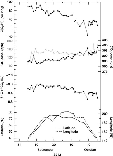
Fig. 3 Same as in Fig. 2 but for the period 29 August–6 October 2013.

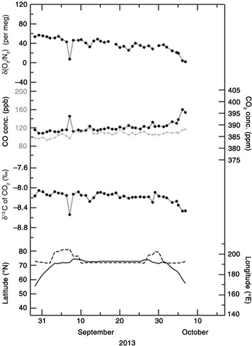
Fig. 4 Same as in Fig. 2 but for the period 1 September–9 October 2014.

To explore possible driver(s) of the variations in δ(O₂/N₂), δ¹³C of CO₂ and CO₂ concentration, we show the relationships of δ(O₂/N₂) and δ¹³C of CO₂ with CO₂ concentration in Fig. 5, respectively. By applying linear regression analyses to the δ(O₂/N₂) and CO₂ concentration values observed in 2012, 2013 and 2014, the rates of change in δ(O₂/N₂) with respect to CO₂ were calculated to be −7.3±0.5, −5.7±0.3 and −6.2±0.3 per meg·ppm⁻¹, respectively. On the other hand, rates of −0.041±0.002, −0.046±0.003 and −0.043±0.001 ‰·ppm⁻¹ were obtained when δ¹³C was regressed against the CO₂ concentration values obtained in 2012, 2013 and 2014, respectively. Past studies have indicated that the rate of change in δ¹³C with respect to CO₂ is about −0.05 ‰ ppm⁻¹ for CO₂ exchange between the atmosphere and the terrestrial biosphere, and −0.005 ‰ ppm⁻¹ for exchange between the atmosphere and the ocean (e.g. Keeling et al., 1989; Nakazawa et al., 1997). Therefore, the observed rates of −0.041 to −0.046 ‰ ppm⁻¹ obtained in this study are much closer to the rate expected from the CO₂ exchange between the atmosphere and the terrestrial biosphere.

The above results do not exclude the possibility of influence from fossil fuel combustion however, since the average δ¹³C values in fossil fuels and the terrestrial biosphere are similar and estimated to be about −28 ‰ (e.g. Andres et al., 2000; Ito, 2003). However, we can use CO measurements as an indicator of fossil fuel influence. In Figs. 2–4, CO₂ and CO concentrations are also plotted, measured simultaneously by using a gas chromatograph equipped with an Hg reduction detector (Yashiro et al., 2009). We note that the correlations ranging between 0.20 and 0.36 between CO₂ and CO are not statistically significant (at α=0.02), and the rates of change of CO with respect to CO₂ are lower than 1.0 ppb·ppm⁻¹ on every cruise. However, as reported in previous studies (e.g. Lai et al., 2010; Niwa et al., 2014), much higher change rates of CO/CO₂ (over 10 ppb ppm⁻¹) would be expected if fossil fuel combustion is the main contributor to the variations in the observed CO₂ concentration. Therefore, it would be reasonable to regard terrestrial biospheric activities as the main contributor to the variations in the CO₂ concentration values observed in this study.

If δ(O₂/N₂) also varies mainly due to terrestrial biospheric activities, then the rate of change in δ(O₂/N₂) with respect to CO₂ is expected to be −1.1×(0.2095)⁻¹=−5.3 per meg ppm⁻¹. Here the value of −1.1 is the O₂:CO₂ exchange ratio for terrestrial biospheric activities reported by Severinghaus (1995). Although there are some discussions about the universal validity of the value of −1.1 (e.g. Seibt et al., 2004; Masiello et al., 2008; Worrall et al., 2013; Ishidoya et al., 2015), we assume the value of −1.1 throughout this study. The observed rates of change in δ(O₂/N₂) with respect to CO₂ concentration (−7.3±0.5 to −5.7±0.3 per meg ppm⁻¹) obtained in this study are lower than −5.3 per meg ppm⁻¹ that would be expected from terrestrial biospheric activities alone. This could result due to contributions from the air–sea O₂ and N₂ fluxes, as well as from fossil fuel combustion, since the O₂:CO₂ exchange ratio from the combustion of liquid fuel (−1.44) and gases (−1.95) are lower than −1.1 (e.g. Keeling, 1988; Steinbach et al., 2011). However, based on the evidence given in the previous paragraph, we conclude that the observed change rate of δ(O₂/N₂)/CO₂ can be attributed to the air–sea exchange of O₂ and N₂ rather than to fossil fuel combustion.

3.2. APO and air–sea O₂ fluxes observed onboard a research vessel MIRAI

Following the discussion in Section 3.1, we can extract the oceanic component from the measured values of δ(O₂/N₂) by using APO defined by eq. (3). The APO values for the periods 5 September–15 October 2012, 29 August–6 October 2013, and 1 September–9 October 2014 are shown in Figs. 6–8, respectively (black filled circles). We have also plotted the APO values calculated from the STAG model driven by F_{O2_cli} and F_{N2_cli} (blue crosses). The average value of the simulated APO for each cruise was adjusted as a function of the differences between F_{O2_obs} and F_{O2_cli} (see discussion below). It can be seen in Figs. 6–8 that the average value of the observed APO decreases from 2012 to 2014. This can be attributed not only to a secular increase in atmospheric CO₂ due to fossil fuel combustion for which the average O₂:CO₂ exchange ratio (about −1.4) is lower than that of the terrestrial biospheric activity (−1.1), but also to a secular oceanic CO₂ uptake. It can also be seen from Figs. 6–8 that the observed APO values decrease gradually with time for each cruise. This decrease from September to October has been widely observed in the Northern Hemisphere in other studies (e.g. Keeling et al., 1998; Tohjima et al., 2012), and reflects seasonal changes in the air–sea O₂ flux. While the simulated APO values show similar seasonal decreasing trend in APO for each cruise, the observed day-to-day variation is significantly underestimated by the model. This underestimation could be due to the difference between F_{O2_cli} used to drive the model and the actual air–sea O₂ flux used to calculate the observed APO. In order to show this to be the case, we have also plotted in Figs. 6–8 F_{O2_obs} and F_{O2_cli} for each cruise.

Fig. 5 Relationships of (a) δ(O₂/N₂) and (b) δ¹³C of CO₂ with CO₂ concentration observed onboard MIRAI for the period 5 September–15 October 2012, 29 August–6 October 2013, and 1 September–9 October 2014.

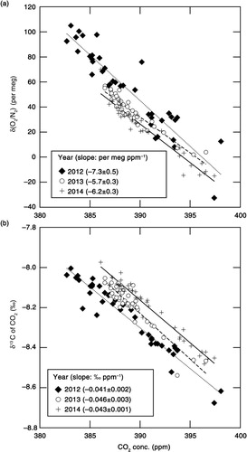
Fig. 6 Temporal variations in APO (filled black circles) and air–sea O₂ flux observed onboard MIRAI (F_{O2_obs}; green dots, positive value denotes flux emitted from the ocean to the atmosphere) for the period 5 September–15 October 2012. Corresponding APO values simulated using the STAG model that incorporated the monthly air–sea O₂ (N₂) flux climatology (blue crosses), and the climatological air–sea O₂ flux along the observation route (F_{O2_cli}; blue dots) are also plotted. Simulated APO values calculated by including the contribution of air–sea CO₂ flux are also shown by the blue dotted line (see text). Green crosses denote temporal variations in APO calculated by using F_{O2_obs} (see text). Chlorophyll-a concentration, partial pressure of O₂ and CO₂ in surface water, heights of planetary boundary layer (PBLH), wind speed at 25-m heights, latitude and longitude of the cruise are also shown.

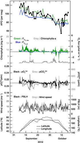
Fig. 7 Same as in Fig. 6 but for the 29 August–6 October 2013.

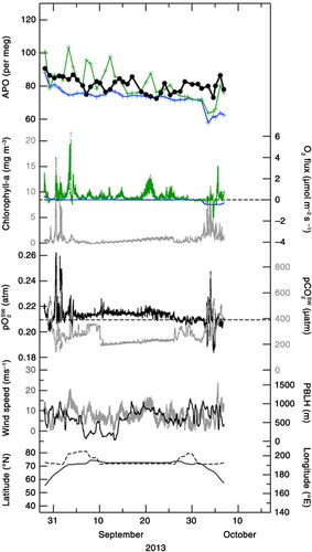
Fig. 8 Same as in Fig. 6 but for the period 1 September–9 October 2014.

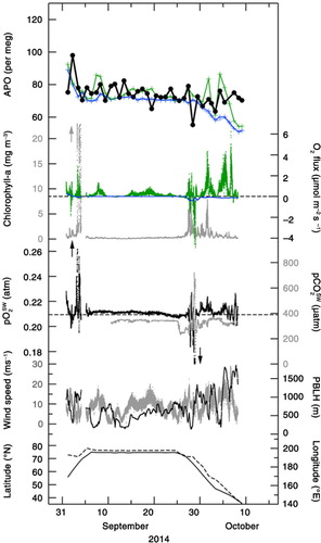
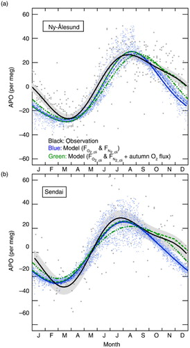
Fig. 9 Seasonal components of the observed APO (grey dots) and the simulated APO (blue dots) by STAG model incorporated with F_{O2_cli} and F_{N2_cli} at (a) Ny-Ålesund, Svalbard, for the period 2001–2010 (Ishidoya et al., 2012a) and (b) Sendai, Japan, for the period 1999–2009 (Ishidoya et al., 2012b). Best-fitted curves to the observed and simulated data consisting of two-harmonics are also shown by black and blue solid lines, respectively. Blue dashed lines denote the same best-fitted curves to the simulated data but for including the contribution of air–sea CO₂ flux. Green dashed lines denote the APO values calculated as a sum of the simulated APO and changes in APO expected from a uniform mixing of the sea-to-air O₂ fluxes, emitted from the northern hemispheric ocean at a uniform rate of 0.3 µmol·m⁻²·s⁻¹ for the period from mid-September to the end of November. Green dashed-dot-dot lines denote the best-fitted curves to the simulated APO produced by the adjusted F_{O2_cli} values. See text for details.

In Figs. 6–8, F_{O2_obs} shows clear short-term (intra- to inter-diurnal) variations, while F_{O2_cli} does not. It can be seen that many positive peaks (i.e. emitted from the ocean to the atmosphere) larger than 1 µmol·m⁻²·s⁻¹ are associated with F_{O2_obs} , while F_{O2_cli} values are always lower than 0.4 µmol·m⁻²·s⁻¹. F_{O2_obs} is higher by about 0.3 µmol·m⁻²·s⁻¹ than F_{O2_cli} , on average, throughout the study period 2012–2014. These results strongly suggest that the short-term variations detected in the observed APO are likely due to the short-term variations in F_{O2_obs} , as well as the fact that the simulated APO calculated by using F_{O2_cli} underestimates the actual APO systematically. Furthermore, as shown in Figs. 6–8, when F_{O2_obs} are positive, values are larger than the partial pressure of O₂ in air (, ~0.2095 atm), with variations in F_{O2_obs} to be dependent on variations in and wind speeds (also plotted in Figs. 6–8). In addition, temporal variations in the observed APO and resemble each other in shape, especially in 2012 and 2014. These results provide additional evidence that the variation in is one of the contributing factors in generating temporal variations in the observed APO. In Figs. 6–8, we also plotted the simulated APO values (blue dotted lines) that included the contribution of APO_{CO2_oc} . The differences between the simulated APO values with or without including the APO_{CO2_oc} are very small (0.5 per meg on average). This means that the contribution from the air–sea CO₂ flux to the short-term variations in APO is negligibly smaller than those from the air–sea O₂ and N₂ fluxes, as expected from the relationship between CO₂ and δ¹³C of CO₂ discussed above.

In order to provide a quantitative support for our suggested relationship between the observed APO and F_{O2_obs} , we used a simple model that assumed a well-mixed planetary boundary layer (PBL). Then, that portion of F_{O2_obs} that remained after deducting F_{O2_cli} was uniformly mixed into a column of air extended from the surface to PBL height (PBLH) over a 24-hour period (before and after 12 hours relative to the observation time). The PBLH values were taken from the ECMWF ERA-interim reanalysis datasets (Dee et al., 2011) and plotted in Figs. 6–8. Thus calculated values are added to the simulated APO by the STAG model driven by F_{O2_cli} and F_{N2_cli} , and shown by green crosses in Figs. 6–8 (hereafter referred to as the ‘APO calculated by using F_{O2_obs} ’). As mentioned above for the purpose of display, the average values of the simulated APO by STAG have been adjusted to equalise the average values of the observed APO to those of the APO calculated by using F_{O2_obs} for the respective cruises.

Standard deviations (SD) of the observed APO, the APO calculated by using F_{O2_obs} and the APO simulated by using F_{O2_cli} from their respective 4-d running mean values were calculated to be 4, 5 and 1 per meg, respectively, throughout the observation period. Therefore, the short-term variations in APO calculated by using F_{O2_obs} are comparable in magnitude to those in the observed APO but larger than those simulated by using F_{O2_cli} . This result is not changed even if we consider the possible overestimation of F_{O2_obs} in this study due to the bubble effects, since the above-mentioned SD of the APO calculated by using F_{O2_obs} is reduced by only 20 % (changed from 5 to 4 per meg)by considering the largest bubble effects (see Methods). Furthermore, the gradual decrease in September and the slight increase in October in the observed APO are relatively well reproduced in the calculated APO using F_{O2_obs} .

We have also confirmed, based on a backward trajectory analyses using HYSPLIT (Draxler and Rolph, 2003; Rolph, 2003; available from NOAA Air Resources Laboratory at www.ready.arl.noaa.gov/HYSPLIT_traj.php), that the average transport distance of an air parcel for 1-d backward trajectories is roughly about 500 km from the ship. Therefore, it is likely that the short-term variations seen in the observed APO are influenced by the variations in the air–sea O₂ flux within a few hundred kilometers from the ship; therefore, F_{O2_obs} has a certain level of regional representativeness. These results imply that a shipboard observation of APO will be a useful constraint for estimating the regional air–sea O₂ flux by an inversion analysis, and that a shipboard observation of F_{O2_obs} will be useful to validate the estimated air–sea O₂ flux. Estimating regional air–sea O₂ fluxes would also be important for evaluating regional marine biological activities. We plotted the partial pressure of CO₂ in surface water () observed onboard MIRAI (Kosugi et al., submitted to Geophys. Res. Lett.) in Figs. 6–8. The values are generally smaller than the partial pressure of CO₂ in air (, ~390 µatm in this study), and vary roughly in opposite phase with . This suggests that > observed in this study, which yields positive F_{O2_obs} , is at least partly attributable to super- and under-saturation of O₂ and CO₂, respectively, caused by marine biological activities. In addition, some local maxima in chlorophyll-a concentration (measured by a fluorometer and calibrated by water-sampled chlorophyll-a data using the fluorometric non-acidification method (Welschmeyer, 1994; see the MIRAI cruise reports in detail)) in the surface water observed onboard MIRAI (also plotted in Figs. 6–8) show a correlation with some local maxima, as well as with positive peaks of F_{O2_obs} . This indicates that marine biological activities are one of the significant drivers of F_{O2_obs} . Therefore, an inversion analysis by using ship-based APO is expected to be a useful tool to constrain regional ocean productivity, as Thompson et al. (2008) obtained rough estimates of regional marine net community production based on their ship-based observation by assuming that biology is the principle driver of air–sea O₂ fluxes.

Our results indicate that the simulated APO driven by F_{O2_cli} underestimates the actual APO systematically. Although the region we observed in this study appears to have minimal contribution to the overall global air–sea O₂ flux, if we assume boldly that such an underestimation of the O₂ outflux (or overestimation of the O₂ influx) in F_{O2_cli} is relatively common in other locations in the Northern Hemisphere in the autumn, then it is expected that a decreasing rate in APO from summer to winter will be more rapid in the seasonal cycle of the simulated APO using F_{O2_cli} than that in the observed seasonal APO cycle. Figure 9 shows a comparison between average seasonal components of the observed and simulated APO at Ny-Ålesund (79 °N, 12 °E), Svalbard for the period 2001–2010 (Ishidoya et al., 2012a) and Sendai (38 °N, 140 °E), Japan for the period 1999–2009 (Ishidoya et al., 2012b). Best-fitted curves to the observed and simulated data consisting of two-harmonics are also shown. The error bands of the fitted curves to the observed data are evaluated by a similar bootstrap method used in Ishidoya et al. (2012a) (Press et al., 2007). The locations of Ny-Ålesund and Sendai are shown in Fig. 1. In Fig. 9, clear discrepancies in the fall-time temporal decreasing rates of APO can be seen between the observed and simulated APO at both sites. Similar discrepancies are widely seen in the seasonal APO cycles observed at other locations in the Northern Hemisphere (e.g. Battle et al., 2006; Tohjima et al., 2012). In Fig. 9, the best-fitted curves to the simulated APO that included the contribution of APO_{CO2_oc} are also shown (blue dashed lines). The seasonal cycles of the simulated APO without the contribution of APO_{CO2_oc} are found to be slightly different from those including the contribution, however the differences are much smaller than the fall-time discrepancies between the observed and simulated APO. Therefore, it is suggested that the discrepancy between the observed and simulated seasonal APO cycles is mainly attributable to an uncertainty of F_{O2_cli} rather than that of the air–sea CO₂ flux.

To examine the potential impact of the underestimation of F_{O2_cli} during the fall season, we simply calculated changes in APO expected when a uniformly distributed O₂ flux of 0.3 µmol·m⁻²·s⁻¹ is emitted into a well-mixed northern hemispheric air from mid-September to the end of November. For the calculation, the total global dry air mass of 5.124×10²¹ g was taken from Trenberth (1981) and a mean molecular weight of dry air was assumed to be 29 g mol⁻¹. Then, the calculated fall-time changes in APO were simply added to the best-fitted curves of the simulated APO at Ny-Ålesund and Sendai shown in Fig. 9. The resultant curves, indicated by the green dashed lines in Fig. 9, show similar decreasing rates in the fall as seen in the observed seasonal APO cycles, giving support to our suggestion that F_{O2_cli} underestimates the fall-time fluxes by about 0.3 µmol·m⁻²·s⁻¹ on average in the Northern Hemisphere. A corollary analysis was conducted by running STAG driven by the adjusted F_{O2_cli} values. In this experiment, the northern hemispheric F_{O2_cli} values were enhanced by 0.3 µmol·m⁻²·s⁻¹ uniformly from early September to mid-November, and then an arbitrary constant value was subtracted from the global F_{O2_cli} values to adjust the globally integrated annual mean F_{O2_cli} to zero. The best-fitted curves to the simulated APO produced by the adjusted F_{O2_cli} , indicated by the green dashed–two dotted lines in Fig. 9, match the observed fall-time enhancement of APO relative to those simulated by using F_{O2_cli} . However, the seasonal maxima and summer-to-fall decreasing rates found in the simulated APO driven by the adjusted F_{O2_cli} appear later and steeper, respectively, than those in the observed seasonal APO cycles. These results suggest that the discrepancies between the seasonal cycles of the observed APO and the simulated APO driven by F_{O2_cli} cannot be entirely attributed to the underestimation of F_{O2_cli} during the fall season, because the wintertime (December to February) decreasing rates seen in the observed seasonal APO cycles are clearly larger than those seen in the simulated APO.

Causes of the suggested underestimation of F_{O2_cli} may be related to its calculation method, which is based on a linear regression analysis between the air–sea O₂ flux and the air–sea heat flux in 10 ° latitudinal bands covering the entire ice-free world ocean. Therefore, it is expected that the method would fail to capture that part of the air–sea O₂ flux (such as the one discussed in the paper) unrelated to the air–sea heat flux process. The total flux should include the influence due to a fall-time intrusion of biologically produced shallow oxygen maximum (SOM) to the surface due to the deepening of the mixed layer in the autumn (e.g. Shulenberger and Reid, 1981; Riser and Johnson, 2008). This process is not linearly related to the air–sea heat flux. In this regard, Nishino et al. (2015) reported that a clear SOM was observed in the Arctic Ocean in 2013 during the same MIRAI cruise discussed in this study, especially in the shelf break of Chukchi Sea. They concluded that the observed SOM was not produced by a local phytoplankton growth during the observation period, but might be a remnant of a previous phytoplankton bloom and/or resulted from the spread of O₂ rich water from the Canada Basin. Therefore, the parameterisation of air–sea O₂ flux may be improved by using some biological components, such as chlorophyll-a concentration from satellite observations, in combination with the air–sea heat flux.

4. Conclusions

Atmospheric δ(O₂/N₂), CO₂ concentration and δ¹³C of CO₂ were observed onboard R/V MIRAI in the northern North Pacific and the Arctic Ocean during the autumn seasons of 2012–2014. Dissolved oxygen concentration in the near-surface water was also measured continuously during these cruises, and converted to air–sea O₂ flux (F_{O2_obs} ). The relationships of δ(O₂/N₂) and δ¹³C with CO₂ concentration indicated that terrestrial biospheric processes and the air–sea O₂ flux are the main contributors to the observed variations in CO₂ concentration and APO, respectively.

To compare the observed APO values with those simulated using the monthly air–sea O₂ flux climatology taken from the TransCom experimental protocol (F_{O2_cli} ), a simulation of APO using the STAG three-dimensional atmospheric transport model forced by F_{O2_cli} was also carried out. The observed APO showed larger short-term variations than the simulated APO forced by F_{O2_cli} , and F_{O2_obs} also showed larger variation than F_{O2_cli} . A simple calculation indicated that the short-term variations in APO produced by using F_{O2_obs} were comparable in magnitude to the observed, and the characteristics of the temporal variations in the observed APO were relatively well reproduced by the calculated APO. We conclude that the short-term variations seen in the observed APO are attributable to the short-term variations in the air–sea O₂ flux around the observation area. The F_{O2_obs} values were systematically higher than the F_{O2_cli} values in all cruises, with an average difference of about 0.3 µmol·m⁻²·s⁻¹. By uniformly mixing the sea-to-air O₂ flux of 0.3 µmol·m⁻²·s⁻¹ from the Northern Hemisphere ocean into the overlying atmosphere during the fall season, it was possible to account for the discrepancies in the APO decreasing rates between the observed and simulated seasonal APO cycles at Ny-Ålesund and Sendai.

The results of the present study show that simultaneous ship observations of APO and F_{O2_obs} can be a powerful tool for detailed validation of regional air–sea O₂ fluxes, since we can examine the validity of the air–sea O₂ flux inferred by an inversion of APO in comparison with F_{O2_obs} . If it is confirmed that the inversion of APO is valid to estimate the regional air–sea O₂ flux, then ship observations of APO is expected to be useful for estimating the regional ocean productivity and mixing, since their changes drive the regional air–sea O₂ fluxes.

5. Acknowledgements

We thank the captain, crew and technical staffs of R/V MIRAI for their hard work in collecting the data and samples. We also thank J. Matsushita and K. Katsumata (National Institute for Environmental Studies) for their support to collect the data and samples. This study was partly supported by GRENE Arctic Climate Change Research Project.

References

- Andres R. J. , Marland G. , Boden T. , Bischof S . Wigley T. M. L. , Schimel D. S . Carbon dioxide emissions from fossil fuel consumption and cement manufacture, 1751–1991, and an estimate of their isotopic composition and latitudinal distribution. The Carbon Cycle. 2000; Cambridge University Press, Cambridge. 53–62.
- Battle M. , Bender M. L. , Tans P. P. , White J. W. C. , Ellis J. T. , co-authors . Global carbon sinks and their variability inferred from atmospheric O2 and δ13C. Science. 2000; 287: 2467–2470.
- Battle M., Fletcher S., Bender M., Keeling R., Manning A., co-authors. Atmospheric potential oxygen: new observations and their implications for some atmospheric and oceanic models. Glob. Biogeochem. Cycles. 2006; 20: 1010. DOI: http://dx.doi.org/10.1029/2005GB002534.
- Bender M. L., Ho D. T., Hendricks M. B., Mika R., Battle M. O., co-authors. Atmospheric O2/N2 changes, 1993–2002: implications for the partitioning of fossil fuel CO2 sequestration. Glob. Biogeochem. Cycles. 2005; 19: 4017. DOI: http://dx.doi.org/10.1029/2004GB002410.
- Benson B. B. , Krause O . The concentration and isotopic fractionation of oxygen dissolved in freshwater and seawater in equilibrium with the atmosphere. Limnol. Oceanogr. 1984; 10: 264– 277.
- Blaine T. W . Continuous measurements of atmospheric argon/nitrogen as a tracer of air–sea heat flux: models, methods, and data. 2005; San Diego: PhD Thesis. University of California.
- Buitenhuis E. T., Le Quéré C., Aumont O., Beaugrand G., Bunker A., co-authors. Biogeochemical fluxes through mesozooplankton. Glob. Biogeochem. Cycles. 2005; 20: 2003. DOI: http://dx.doi.org/10.1029/2005GB002511.
- Cassar N., Mckinley G. A., Bender M. L., Mika R., Battle M. An improved comparison of atmospheric Ar/N2 time series and paired ocean–atmosphere model predictions. J. Geophys. Res. 2008; 113: D21122. DOI: http://dx.doi.org/10.1029/2008JD009817.
- Dee D. P. , Uppala S. M. , Simmons A. J. , Berrisford P. , Poli P. , co-authors . The ERA-Interim reanalysis: configuration and performance of the data assimilation system. Q. J. R. Meteorol. Soc. 2011; 137: 553–597.
- Dickson A. D . Determination of dissolved oxygen in sea water by Winkler titration. WOCE Operations Manual, WHP Operations and Methods. 1996; WHPO 91-1, WOCE Int. Project Office, WOCE Rep. 68/91. 13.
- Draxler R. R., Rolph G. D. HYSPLIT (HYbrid Single-Particle Lagrangian Integrated Trajectory) Model access via NOAA ARL READY Website. 2003; Silver Spring, MD: NOAA Air Resources Laboratory. Online at: http://www.arl.noaa.gov/HYSPLIT.php.
- Garcia H. , Gordon L . Oxygen solubility in seawater: better fitting equations. Limnol. Oceanogr. 1992; 37: 1307–1312.
- Garcia H. , Keeling R . On the global oxygen anomaly and air–sea flux. J. Geophys. Res. 2001; 106(C12): 31155–31166.
- Heimann M. , Körner S . The Global Atmospheric Tracer Model TM3. 2003; Technical Report 5. Max Planck Institute for Biogeochemistry, Jena, Germany.
- Ishidoya S., Aoki S., Goto D., Nakazawa T., Taguchi S., co-authors. Time and space variations of the O2/N2 ratio in the troposphere over Japan and estimation of global CO2 budget. Tellus B. 2012b; 64: 18964. DOI: http://dx.doi.org/10.3402/tellusb.v64i0.18964.
- Ishidoya S., Morimoto S., Aoki S., Taguchi S., Goto D., co-authors. Oceanic and terrestrial biospheric CO2 uptake estimated from atmospheric potential oxygen observed at Ny-Alesund, Svalbard, and Syowa, Antarctica. Tellus B. 2012a; 64: 18924. DOI: http://dx.doi.org/10.3402/tellusb.v64i0.18924.
- Ishidoya S., Murayama S. Development of high precision continuous measuring system of the atmospheric O2/N2 and Ar/N2 ratios and its application to the observation in Tsukuba, Japan. Tellus B. 2014; 66: 22574. DOI: http://dx.doi.org/10.3402/tellusb.v66.22574.
- Ishidoya S. , Murayama S. , Kondo H. , Saigusa N. , Kishimoto-Mo A. W. , co-authors . Observation of O2:CO2 exchange ratio for net turbulent fluxes and its application to forest carbon cycles. Ecol. Res. 2015; 30: 225–224.
- Ito A . A global-scale simulation of the CO 2 exchange between the atmosphere and the terrestrial biosphere with a mechanistic model including stable carbon isotopes, 1953–1999. Tellus B. 2003; 55: 596–612.
- Keeling C. D. , Bacastow R. B. , Carter A. F. , Piper S. C. , Whorf T. P. , co-authors . A three-dimensional model of atmospheric CO2 transport based on observed winds: 1. Analysis of observational data. Geograph. Monogr. 1989; 55: 165–236.
- Keeling R. F . Development of an interferometric oxygen analyzer for precise measurement of the atmospheric O2 mole fraction. 1988; Cambridge: PhD Thesis. Harvard University.
- Keeling R. F. , Bender M. L. , Tans P. P . What atmospheric oxygen measurements can tell us about the global carbon cycle. Global Biogeochem Cycles. 1993; 7: 37–67.
- Keeling R. F. , Manning A . Holland H. , Turekian K . Studies of recent changes in atmospheric O2 content. Treatise on Geochemistry. 2014; Elsevier, Amsterdam, Netherlands. 385–405.
- Keeling R. F. , Piper S. C. , Heimann M . Global and hemispheric CO2 sinks deduced from changes in atmospheric O2 concentration. Nature. 1996; 381(6579): 218–221.
- Keeling R. F. , Stephens B. B. , Najjar R. G. , Doney S. C. , Archer D. , co-authors . Seasonal variations in the atmospheric O2/N2 ratio in relation to the kinetics of air–sea gas exchange. Global Biogeochem Cycles. 1998; 12: 141–163.
- Kozlova E. A., Manning A. C., Kisilyakhov Y., Seifert T., Heimann M. Seasonal, synoptic, and diurnal-scale variability of biogeochemical trace gases and O2 from a 300-m tall tower in central Siberia. Glob. Biogeochem. Cycles. 2008; 22: GB4020. DOI: http://dx.doi.org/10.1029/2008GB003209.
- Lai S. C. , Baker A. K. , Schuck T. J. , van Velthoven P. , Oram D. E. , co-authors . Pollution events observed during CARIBIC flights in the upper troposphere between South China and the Philippines. Atoms. Chem. Phys. 2010; 10: 1649–1660.
- Langenfelds R. L. , Francey R. J. , Steel L. P. , Battle M. , Keeling R. F. , co-authors . Partitioning of the global fossil CO2 sink using a 19-year trend in atmospheric O2 . Geophys. Res. Lett. 1999; 26: 1897–1900.
- Machta L. , Hughes E . Atmospheric oxygen in 1967 to 1970. Science. 1970; 168: 1582–1584.
- Maksyutov S. , Inoue G . Shimizu H . Vertical profiles of radon and CO2 simulated by the global atmospheric transport mode. CGER Supercomputer Activity Report, 1039–2000. 2000; CGER NIES, Tsukuba, Japan. 39–41.
- Manning A. C. , Keeling R. F . Global oceanic and terrestrial biospheric carbon sinks from the Scripps atmospheric oxygen flask sampling network. Tellus B. 2006; 58: 95–116.
- Masiello C. A., Gallagher M. E., Randerson J. T., Deco R. M., Chadwick O. A. Evaluating two experimental approaches for measuring ecosystem carbon oxidation state and oxidative ratio. J. Geophys. Res. 2008; 113: G03010. DOI: http://dx.doi.org/10.1029/2007JG000534.
- Najjar R. G. , Keeling R. F . Mean annual cycle of the air-sea oxygen flux: A global view. Glob. Biogeochem. Cycles. 2000; 14(2): 573–584.
- Nakazawa T. , Morimoto S. , Aoki S. , Tanaka M . Time and space variations of the carbon isotopic ratio of tropospheric carbon dioxide over Japan. Tellus B. 1993; 45: 258–274.
- Nakazawa T. , Morimoto S. , Aoki S. , Tanaka M . Temporal and spatial variations of the carbon isotopic ratio of atmospheric carbon dioxide in the western Pacific region. J. Geophys. Res. 1997; 102: 1271–1285.
- Nevison C. D., Keeling R. F., Kahru M., Manizza M., Mitchell B. G., co-authors. Estimating net community production in the Southern ocean based on atmospheric potential oxygen and satellite ocean color data. Glob. Biogeochem. Cycles. 2012; 26: GB1020. DOI: http://dx.doi.org/10.1029/2011GB004040.
- Nishino S., Kawaguchi Y., Inoue J., Hirawake T., Fujiwara A., co-authors. Nutrient supply and biological response to wind-induced mixing, inertial motion, internal waves, and currents in the northern Chukchi Sea. J Geophys. Res. 2015; 120: 1975–1992. DOI: http://dx.doi.org/10.1002/2014JC010407.
- Niwa Y., Tsuboi K., Matsueda H., Sawa Y., Machida T., co-authors. Seasonal variations of CO2, CH4, N2O and CO in the mid-troposphere over the western North Pacific observed using a C-130H cargo aircraft. J. Meteorol. Soc. Jpn. 2014; 92: 55–70. DOI: http://dx.doi.org/10.2151/jmsj.2014-104.
- Press W. H. , Teukolsky S. A. , Vetterling W. T. , Flannery B. P . Numerical Recipes: The Art of Scientific Computing. 2007; New York, NY: Cambridge University Press.
- Riser S. C., Johnson K. S. Net production of oxygen in the subtropical ocean. Nature. 2008; 451(17): 323–325. DOI: http://dx.doi.org/10.1038/nature06441.
- Rödenbeck C. , Le Quéré C. , Heimann M. , Keeling R. F . Interannual variability in oceanic biogeochemical processes inferred by inversion of atmospheric O2/N2 and CO2 data. Tellus B. 2008; 60: 685–705.
- Rolph G. D. Real-time Environmental Applications and Display sYstem (READY) Website. 2003; Silver Spring, MD: NOAA Air Resources Laboratory. Online at: http://www.arl.noaa.gov/ready.php.
- Seibt U., Brand W. A., Heimann M., Lloyd J., Severinghaus J. P., co-authors. Observations of O2:CO2 exchange ratios during ecosystem gas exchange. Glob. Biogeochem. Cycles. 2004; 18: GB4024. DOI: http://dx.doi.org/10.1029/2004GB002242.
- Severinghaus J . Studies of the terrestrial O2 and carbon cycles in sand dune gases and in biosphere 2. 1995; Columbia University, New York, NY: PhD Thesis.
- Shulenberger E. , Reid J. L . The Pacific shallow oxygen maximum, deep chlorophyll maximum, and primary productivity, reconsidered. Deep. Sea. Res. 1981; 28A: 901–919.
- Steinbach J. , Gerbig C. , Rodenbeck C. , Karstens U. , Minejima C. , co-authors . The CO2 release and Oxygen uptake from Fossil Fuel Emission Estimate (COFFEE) dataset: effects from varying oxidative ratios. Atmos. Chem. Phys. 2011; 11: 6855–6870.
- Stephens B. B. , Keeling R. F. , Heimann M. , Six K. , Murnane R. , co-authors . Testing global ocean carbon cycle models using measurements of atmospheric O2 and CO2 concentration. Glob. Biogeochem. Cycles. 1998; 12: 213–230.
- Stephens B. B. , Keeling R. F. , Paplawsky W. J . Shipboard measurements of atmospheric oxygen using a vacuum-ultraviolet absorption technique. Tellus B. 2003; 55: 857–878.
- Taguchi S . A three-dimensional model of atmospheric CO2 transport based on analyzed winds: model description and simulation results for TRANSCOM. J. Geophys. Res. 1996; 101(D10): 15099–15110.
- Taguchi S. , Matsueda H. , Inoue H. Y. , Sawa Y . Long-range transport of CO from tropical ground to upper troposphere: a case study for Southeast Asia in October 1997. Tellus B. 2002; 54: 22–40.
- Takahashi T. , Sutherland S. C. , Sweeney C. , Poisson A. , Metzl N. , co-authors . Global sea–air CO2 flux based on climatological surface ocean pCO2, and seasonal biological and temperature effects. Deep Sea Res. II. 2002; 49: 1601–1622.
- Takahashi T., Sutherland S. C., Wanninkhof R., Sweeney C., Feely R. A., co-authors. Climatological mean and decadal change in surface ocean pCO2, and net sea–air CO2 flux over the global oceans. Deep Sea Res. II. 2009; 56: 554–577. DOI: http://dx.doi.org/10.1016/j.dsr2.2008.12.009.
- Tanaka M. , Nakazawa T. , Aoki S . High quality measurements of the concentration of atmospheric carbon dioxide. J. Meteorol. Soc. Jpn. 1983; 61: 678–685.
- Thompson R. L. , Manning A. C. , Lowe D. C. , Wetherburn D. C . A ship-based methodology for high precision atmospheric oxygen measurements and its application in the Southern Ocean region. Tellus B. 2007; 59: 643–653.
- Thompson R. L., Gloor M., Manning A. C., Lowe D. C., Rödenbeck C., co-authors. Variability in atmospheric O2 and CO2 concentrations in the southern Pacific Ocean and their comparison with model estimates. J. Geophys. Res. 2008; 113: G02025. DOI: http://dx.doi.org/10.1029/2007JG000554.
- Tohjima Y., Minejima C., Mukai H., Machida T., Yamagishi H., co-authors. Analysis of seasonality and annual mean distribution of the atmospheric potential oxygen (APO) in the Pacific region. Glob. Biogeochem. Cycles. 2012; 26: GB4008. DOI: http://dx.doi.org/10.1029/2011GB004110.
- Tohjima Y., Mukai H., Machida T., Nojiri Y. Gas-chromatographic measurements of the atmospheric oxygen/nitrogen ratio at Hateruma Island and Cape Ochi-Ishi, Japan. Geophys. Res. Lett. 2003; 30: 1653. DOI: http://dx.doi.org/10.1029/2003GL01782.
- Tohjima Y., Mukai H., Machida T., Nojiri Y., Gloor M. First measurements of the latitudinal atmospheric O2 and CO2 distributions across the western Pacific. Geophys. Res. Lett. 2005; 32: L17805. DOI: http://dx.doi.org/10.1029/2005GL023311.
- Tohjima Y. , Mukai H. , Nojiri Y. , Yamagishi H. , Machida T . Atmospheric O2/N2 measurements at two Japanese sites: estimation of global oceanic and land biotic carbon sinks and analysis of the variations in atmospheric potential oxygen (APO). Tellus B. 2008; 60: 213–225.
- Tohjima Y., Terao Y., Mukai H., Machida T., Nojiri Y., co-authors. ENSO-related variability in latitudinal distribution of annual mean atmospheric potential oxygen (APO) in the equatorial Western Pacific. Tellus B. 2015; 67: 25869. DOI: http://dx.doi.org/10.3402/tellusb.v67.25869.
- Trenberth K. E . Seasonal variations in global sea level pressure and the total mass of the atmosphere. J Geophys. Res. 1981; 86(C6): 5238–5246.
- Uchida H., Johnson G. C., McTaggart K. E. CTD Oxygen Sensor Calibration Procedures. 2010. IOCCP Report. 14, International CLIVAR Project Office (ICPO) Publication Series, 134(1). Online at: http://www.clivar.org/about/icpo.
- Uchida H., Katsumata K., Doi T. WHP P14S, S04I Revisit in 2012 Data Book. 2015; Yokosuka, Kanagawa, Japan: JAMSTEC. Online at: http://www.jamstec.go.jp/iorgc/ocorp/data/s04irev_2012/.
- van der Laan S. , van der Laan-Luijk I. T. , Rödenbeck C. , Varlagin A. , Shironya I. , co-authors . Atmospheric CO2, (δO2/N2), APO and oxidative ratios from aircraft flask samples over Fyodorovskoye, Western Russia. Atmos. Environ. 2014; 97: 174–181.
- Wanninkhof R . Relation between wind speed and gas exchange over the ocean. J. Geophys. Res. 1992; 97: 7337–7382.
- Weiss R. F. , Price B. A . Nitrous oxide solubility in water and seawater. Marine Chemistry. 1980; 8: 347–359.
- Welschmeyer N. A . Fluorometric analysis of chlorophyll a in the presence of chlorophyll b and pheopigments. Limnor Oceanogr. 1994; 39: 1985–1992.
- Wong G. T. F. , Li K.-Y . Winkler's method overestimates dissolved oxygen in seawater: iodate interference and its oceanographic implications. Marine Chemistry. 2009; 115: 86–91.
- Worrall F., Clay G. D., Masiello C. A., Mynheer G. Estimating the oxidative ratio of the global terrestrial biosphere carbon. Biogeochemistry. 2013; 115: 23–32. DOI: http://dx.doi.org/10.1007/s10533-013-9877-6.
- Yashiro H., Sugawara S., Sudo K., Aoki S., Nakazawa T. Temporal and spatial variations of carbon monoxide over the western part of the Pacific Ocean. J. Geophys. Res. 2009; 114: D08305. DOI: http://dx.doi.org/10.1029/2008JD010876.