Air–sea gas exchange in the North Atlantic: ³He/SF₆ experiment during GasEx-98

Abstract

GasEx-98 was the first open-ocean process study where gas transfer velocity measurements were made with several robust techniques, including airside eddy covariance of CO₂ and deliberate injection of ³He and SF₆. While the CO₂ eddy covariance results have been fully analysed and publicised, leading to a boom in the use of this technique in the marine environment, the ³He/SF₆ results have not received the same level of analysis. Here, based on new approaches that we have developed to analyse ³He/SF₆ data in the subsequent years, we revisit the ³He/SF₆ dual tracer results from GasEx-98 and show that they are consistent with the results from other parts of the coastal and open ocean, and that they are in agreement with current parameterisations between wind speed and gas exchange for slightly soluble gases over the ocean at intermediate wind speeds.

• air–sea gas exchange
• ³He/SF₆ dual tracer technique
• North Atlantic

To access the supplementary material to this article, please see Supplementary files under ‘Article Tools’.

1. Introduction

Air–sea gas exchange plays a major role in the cycling of biogeochemically important trace gases, such as CO₂ and DMS, between the atmosphere and the ocean, and in turn affects the climate of our planet. As such, great efforts have been made to study the factors that influence air–sea gas exchange and relate the rate of gas exchange to environmental processes that can be easily observed. Research so far has shown wind speed to be the best correlate for gas exchange, as wind produces near surface turbulence and bubbles, two of the main mechanisms responsible for regulating air–sea gas exchange.

Until about 25 years ago, our understanding of the relationship between wind speed and air–sea gas exchange relied on studies that used the mass balance of opportunistic tracers such as ²²²Rn (Peng et al., 1979) and thermonuclear bomb produced ¹⁴C (Broecker et al., 1985). Since then, ³He/SF₆ dual tracer experiments have emerged as a robust way to obtain integrated measurements of air–sea gas exchange based on water column measurements in the ocean on short time scales. A series of these experiments have been conducted in both the coastal and open oceans (Watson et al., 1991; Wanninkhof et al., 1993, 1997, 2004; Nightingale et al., 2000a, 2000b; Ho et al., 2006, 2011b; Salter et al., 2011).

The results of these experiments reinforce the view that wind is the dominant process driving air–sea exchange of slightly soluble gases in most environments. Other processes and mechanisms (e.g. rain, convection, bubbles and surfactants) might be of importance under certain circumstances, but these processes are either affected by wind or are not dominant on regional to global scales (Ho et al., 2011b). ³He/SF₆ data from coastal ocean experiments in the North Sea (Nightingale et al., 2000b) and an open ocean in the Southern Ocean (Ho et al., 2006) have also been used to derive two wind speed/gas exchange parameterisations that are very similar (see below). These parameterisations show that wind can account for more than 80% of the variance in all the ³He/SF₆ data (Ho et al., 2011b), demonstrating that wind speed/gas exchange parameterisations obtained in one ocean location can be applied to another and implying that under most circumstances, a universal relationship between wind speed and gas exchange of slightly soluble gases (i.e. those with Ostwald solubility coefficients less than 1, including N₂, O₂, N₂O, CH₄ and CO₂) over the ocean can be used. Thus, with knowledge of wind speeds, measurements of air–water concentration differences can provide robust air–sea flux estimates.

GasEx-98 was the first ³He/SF₆ dual tracer experiment conducted in the open ocean and the first successful deployment of micrometeorological techniques, including CO₂ eddy covariance and gradient methods, for measurement of air–sea gas fluxes in the open ocean. While the CO₂ eddy covariance results have been fully analysed and publicised (Wanninkhof and McGillis, 1999; McGillis et al., 2001a, 2001b), the ³He/SF₆ results have not been analysed at daily resolution. This is partly due to the challenging nature of the results, characterised by occasional rapid changes in ³He/SF₆ ratios and fluctuating mixed layer depths as defined by temperature profiles.

Most of the ³He/SF₆ data for the open ocean are from the Southern Ocean (SOFeX (Wanninkhof et al., 2004), SAGE (Ho et al., 2006), SO GasEx (Ho et al., 2011b)), with only four data points from Northern Hemisphere; all from the North Atlantic, with one from GasEx-98 (McGillis et al., 2001b) and three from DOGEE II (Salter et al., 2011). In the following, based on novel approaches to interpret the data refined over the last 15 years, we revisited and analysed the ³He/SF₆ experiment from GasEx-98, which has been described briefly in McGillis et al. (2001b) and where a 2-week averaged gas transfer velocity based on ³He/SF₆ was presented (see Fig. 3).

2. Methods

2.1. GasEx-98

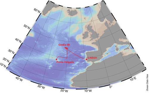
GasEx-98 took place in the North Atlantic in the boreal spring/summer of 1998 (Fig. 1). The experiment consisted of three separate cruises on the NOAA Ship Ronald H. Brown, with the middle leg being a process study in a warm-core ring in the North Atlantic near 46°N and 21.5°W. This leg of the cruise left Lisbon, Portugal on 25 May 1998 (year-day 145) and arrived in Ponta Delgada, Portugal on 26 June 1998 (year-day 177). This portion of the cruise is discussed here and is referred to as GasEx-98. The experiment represents the beginning of the successful GasEx franchise and was followed by GasEx-2001 in the Equatorial Pacific and SO GasEx in the Atlantic sector of the Southern Ocean (McGillis et al., 2001b, 2004; Ho et al., 2011a).

Fig. 1 Map showing the cruise track of the second leg of GasEx-98, where the ³He/SF₆ experiment was conducted. The cruise left from Lisbon, Portugal on 25 May 1998, and arrived in Ponta Delgada, Portugal on 26 June 1998.

2.2. Tracer injection and sampling

On 28 May 1998 (year-day 149), a gaseous mixture of ca. 20 mol of SF₆ and 0.06 mol of ³He was injected as a 5-km streak into the surface mixed layer of a warm core eddy at 15 m depth by bubbling through some diffusion stones. After injection, 614 SF₆ samples and 97 ³He samples were taken from the Niskin bottles over the course of 17 days (from year-days 151 to 167). SF₆ was sampled in 550-ml borosilicate glass bottles with ground glass stoppers, and ³He was sampled in copper tubes mounted in aluminium channels with stainless steel pinch-off clamps. The SF₆ samples were analysed on board the ship using a purge and trap gas chromatographic system equipped with an electron capture detector (Law et al., 1994), while the ³He samples were shipped back to the laboratory, extracted from the copper tubes and analysed on a helium isotope mass spectrometer (Ludin et al., 1998).

In addition to discrete sampling, the surface concentrations of SF₆ were mapped with an underway SF₆ analysis system that measured samples at 2-min intervals. This provided information on the spatial extent and movement of the tracer patch. The discrete samples used in this analysis were those well within the tracer patch to avoid possible biases in the technique caused by secondary dispersion effects.

2.3. Wind speed measurements

Wind speed and direction, along with other meteorological measurements such as air temperature, relative humidity, solar and long-wave radiation, were made at 18 m above sea level using a sonic anemometer on the forward jackstaff of the ship. The high-quality wind speed data were corrected for ship motion and scaled to neutral boundary conditions at 10 m height utilising the measured drag coefficients and taking into account the atmospheric boundary layer stability (Fairall et al., 1996). These robust normalisations to 10 m height and neutral boundary layer conditions removed an often overlooked ambiguity in wind speed measurements that can impact wind speed/gas exchange relationships. Details of the measurement and corrections are given in McGillis et al. (2001a).

2.4. ³He/SF₆ dual tracer technique

With the ³He/SF₆ dual tracer technique, the gas transfer velocity for ³He () can be determined by the change in the ³He/SF₆ ratio with time (Watson et al., 1991; Wanninkhof et al., 1993):1

where h is the depth over which ³He and SF₆ are exchanging with the atmosphere (referred to here as the mixed layer), corresponding to the depth at which the SF₆ reaches 70% of its averaged concentration in the top 12 m. This threshold was chosen based on the depth where SF₆ concentration changes dramatically from the mixed layer value. A comparison of how using a temperature-based mixed layer depth would affect the calculated k is shown in Supplementary File. ³He _exc and SF₆ are the excess ³He concentration (i.e. ³He above solubility equilibrium; use interchangeably here with ³He) and SF₆ concentration in the mixed layer, respectively. The ratios are determined for each depth and then averaged to obtain the profile average. and are the Schmidt numbers (i.e. kinematic viscosity of water, divided by diffusion of gas in water) for SF₆ and ³He, respectively (Wanninkhof, 2014). The gas transfer velocity is then normalised to a Sc of 600, corresponding to that of CO₂ at 20 °C in freshwater:2

Equation (1) can be solved analytically to yield ³He/SF₆ ratio with time, if the initial ³He/SF₆ ratio and the time evolution of h and k(600) are known:3

3. Results and discussion

3.1. ³He and SF₆

After injection, initial excess ³He reached as high as ca. 7000×10⁻¹⁶ ccSTP g⁻¹, from a background level of 2–6×10⁻¹⁶ ccSTP g⁻¹ in the mixed layer, while SF₆ was as high as 180 000 fmol L⁻¹, from a background of ca. 0.6 fmol L⁻¹. Over the course of the experiment, both ³He and SF₆ decreased towards background levels. At the end of the experiment, 18 days after injection, the tracer patch size was estimated to be 15 km in diameter based on the continuous surface SF₆ surveys, and the SF₆ concentrations were still easily detectable at 50 times above background levels. The ³He had decreased to ca. 5–10×10⁻¹⁶ ccSTP g⁻¹ such that the background level correction was important for the measurements towards the end of the experiment.

As with other ³He/SF₆ experiments, the ³He/SF₆ ratios from GasEx-98 do not exhibit a monotonic decrease with time due to differences in fluxes arising from changes in wind speeds. However, there are periods when the ratio decreased more rapidly than can be explained by gas exchange and there are periods when the ratios increased. These rapid changes were most likely due to mixing and mixed layer dynamics as discussed in Ho et al. (2011b). In particular, some of the tracer mixture appeared to have been trapped below the mixed layer during shallowing and isolated from the atmosphere. During intensification of the wind and associated mixed layer deepening, the tracers got re-entrained into the mixed layer. The deepening of the mixed layer and associated mixing of the subsurface chlorophyll maximum and entrainment of nitrate from JD 159–160 when an increase in ³He/SF₆ is observed (Fig. 4) is presented in Hood et al. (2001). Below, we divide our analysis of the ³He/SF₆ time series into six segments, demarcated by station where unrealistic rapid changes in ³He/SF₆ ratios occurred.

3.2. Wind speeds

During the period of the ³He/SF₆ tracer release experiment, wind speeds ranged from 0.8 to 18.3 m s⁻¹, with a mean of 7.1 m s⁻¹ (Fig. 2). The data show that during the experiment, storms moved through the study area in the North Atlantic with a periodicity of roughly 4 days. The wind speed distributions for the six segments differed greatly, with means of ca. 5–11 m s⁻¹ and standard deviations from the mean that varied from 21 to 48% (Table 1).

Fig. 2 Wind speeds measured and adjusted to u ₁₀ on the NOAA Ship Ronald H. Brown during GasEx-98. The shaded areas mark the six segments that were used to evaluate the ³He/SF₆ data.

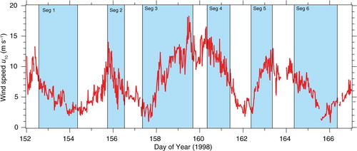
Table 1. Summary of wind speeds and gas transfer velocities from GasEx-98

				Wind Speeds u 10 (m s^−1)							Schmidt numbers^a Sc		Gas transfer velocities^b k(600) (cm h^−1)
Segments	Stations^c	Date range	h ^d (m)	Mean	Range	σ ^e	ɛ ^f	#^g	Temp^h (°C)	Sal^h	^3He	SF6	Mean±error
1	152, 154, 157	152.57–154.36	18.3	4.6	1.9–8.6	1.5	1.11	226	15.11	35.668	175.3	1370.7	7.6±2.7
2	161, 163	155.74–156.53	15.3	7.9	2.9–14.1	2.5	1.10	114	15.41	35.663	173.2	1349.3	18.8±2.8
3	165, 167,169, 171, 172	157.36–159.68	28.6	8.8	0.9–18.3	4.2	1.23	322	15.54	35.657	172.1	1338.5	18.7±3.2
4	173, 176	160.35–161.40	21.7	10.7	1.1–14.9	2.3	1.04	138	15.10	35.657	175.9	1376.5	30.4±4.6
5	178, 179, 180	162.37–163.35	30.8	8.3	2.3–12.8	2.7	1.10	136	15.40	35.670	173.6	1353.8	18.6±8.5
6	184, 190	164.36–166.35	30.0	5.0	0.8–9.3	2.3	1.20	270	15.50	35.679	172.5	1342.8	10.7±1.6

^aAveraged Schmidt numbers of all stations in each segment.

^bEnhancement-corrected k(600) for each segment (i.e. k(600)/ɛ, where ; error in k(600) is determined from the least-squares fit to the ³He/SF₆ decrease for each segment, and the uncertainties in the mixed layer depth.

^cStations in each segment.

^dAveraged mixed layer depth determined from SF₆ profiles.

^eStandard deviation.

^f

^gNumber of 10-minute averaged wind speed measurements in each segment.

^hAveraged temperature and salinity from the surface of all stations in each segment.

3.3. Choice of mixed layer depths

Mixed layer depth has a first order influence on the calculation of k [see eq. (1)]. Different definitions of mixed layer based on temperature or density gradients are available. For purposes of determining k, it is the depth of water exchanging gases with the atmosphere and here we use the depth at which the SF₆ reaches 70 % of its averaged concentration in the top 12 m and call this the tracer mixed layer. This depth is generally less variable than the thermal mixed layer depth (Kim et al., 2005, Fig. 7). The Supplementary File provides an overview of the thermal mixed layer and the tracer mixed layer for each station, and the impact of using the tracer derived mixed layer on determination of k. Internal waves within the eddy caused changes in mixed layer depth up to 5 m over periods of hours that made using thermal mixed layers less reliable. One disadvantage of using the SF₆ profiles is that the sampling for SF₆ was coarse (usually 2–5 m) compared to the CTD (conductivity, temperature, and depth sonde) temperature profile (1 m). The variability in mixed layer depth is a major contributor to the uncertainty in k.

3.4. Gas transfer velocities

Gas transfer velocities were calculated using eq. (1) on the six segments of the ³He/SF₆ time series using the average tracer mixed layer depth between subsequent measurements. Furthermore, these k(600) values [eq. 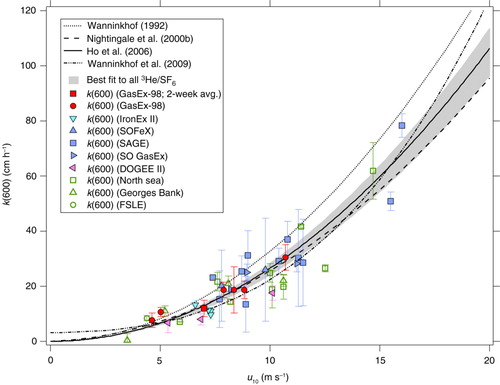(2)] were corrected for enhancement ɛ due to variability in u ₁₀ over each time interval (Wanninkhof et al., 2004) by dividing the resulting k(600) by ɛ, assuming that the relationship between u ₁₀ and k(600) has the functional form of a quadratic (i.e. ). This yields a value of k(600) for instantaneous or steady wind. k(600) varied between 7.6 and 30.4 cm h⁻¹ and is correlated with wind speed (Fig. 3). The k(600) as a function of wind speed for GasEx-98 was similar to other experiments in both the coastal and open oceans referenced above and is in agreement with the 2-week average determined previously from ³He/SF₆ for this study (McGillis et al., 2001b) (Fig. 3).

Fig. 3 Gas transfer velocities for GasEx-98 (filled red circles), corrected to a Schmidt number of 600, plotted along with all published ³He/SF₆ derived k(600) values from the coastal and open oceans against wind speed u ₁₀. The 2-week averaged k(600) presented in McGillis et al. (2001a) is also shown (filled red square). The points for GasEx-98 were determined using a least-squares fit to the ³He/SF₆ ratios from each of the six segments to determine , and then using eqs. (1 and 2) to calculate k(600). The error estimation for the GasEx-98 data is described in the footnotes to Table 1.

3.5. Modelling ³He/SF₆ decrease with different parameterisations

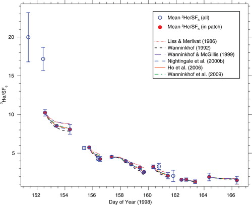
The decrease in ³He/SF₆ ratio during GasEx-98 was modelled using eq. (3). The approach follows the approach first described in Kuss et al. (2004). In short, the time evolution is modelled following a decrease in ³He/SF₆ ratios using one of six commonly used wind speed/gas exchange parameterisations (Liss and Merlivat, 1986; Wanninkhof, 1992; Wanninkhof and McGillis, 1999; Nightingale et al., 2000b; Ho et al., 2006; Wanninkhof et al., 2009) (Fig. 4). The gas exchange/wind speed parameterisations that can represent the decrease best are considered the optimal ones. Each of the six segments was evaluated separately. For each segment, the average tracer mixed layer depth h was determined using the depth profile of SF₆ as described above and detailed in the Supplementary File. The goodness of fit between model and observations were evaluated in terms of relative root mean squared error (rRMSE):4

Fig. 4 Observed and modelled ³He/SF₆ ratio during GasEx-98. Each data point is the mean of the ³He/SF₆ profile from the mixed layer of an individual station, with the error bars representing the standard deviation of ³He/SF₆ in the profile. The open symbols are stations that were not used in the analysis, either because they occurred at the beginning of the experiment before the patch has mixed sufficiently (i.e. the first two stations), or because they were deemed to be outside of the tracer patch based on the surface SF₆ concentrations.

where and are the observed and modelled ³He/SF₆ ratio, respectively, N is the total number of stations in the segment. Table 2 summarises the rRMSE for all six segments. However, we focus our analysis on segments 1 and 3 (Fig. 5). Segments 2, 4 and 6 contain data from only two stations and the fits match one point and therefore have no independent constraint to determine the RMSE [eq. (4)]. Segment 5 contains three stations, but they span less than 1 day. Moreover, for segments 5 and 6, the ³He concentrations were close to background values, increasing the uncertainty in the ³He/SF₆ ratio and therefor the estimation of k(600). However, the results for these intervals are provided in Fig. 3 and are consistent with the analysis below.

Fig. 5 Model and data comparison of ³He/SF₆ ratios for segments 1 and 3 of GasEx-98. For both segments, the parameterisations of Nightingale et al. (2000b), Ho et al. (2006) and Wanninkhof et al. (2009) are most able to model the data.

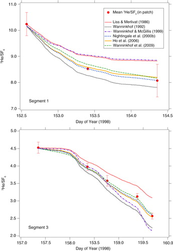
Table 2. Relative root mean square errors of the model/data comparison for each segment of the ³He/SF₆ data for each of the parameterizations listed

	rRMSE
Parameterisations	Segment 1 (%)	Segment 2 (%)	Segment 3 (%)	Segment 4 (%)	Segment 5 (%)	Segment 6 (%)
Liss and Merlivat (1986)	7.8	14.3	11.9	17.3	4.1	15.4
Wanninkhof (1992)	2.5	1.3	9.8	6.7	4.6	6.9
Wanninkhof and McGillis (1999)	8.7	5.5	9.4	10.4	2.7	14.7
Nightingale et al. (2000b)	0.7	7.3	2.1	4.7	2.9	9.8
Ho et al. (2006)	1.8	6.7	2.4	2.3	2.9	10.5
Wanninkhof et al. (2009)	2.2	9.9	1.7	6.9	3.0	10.3

The italicised values are segments 2, 4 and 6 that only contain two stations each, and segment 5, which occurs over the course of less than a day, and have greater measurement uncertainty. The bold values in each segment denote the top 4 parameterisations in terms of having low rRMSE.

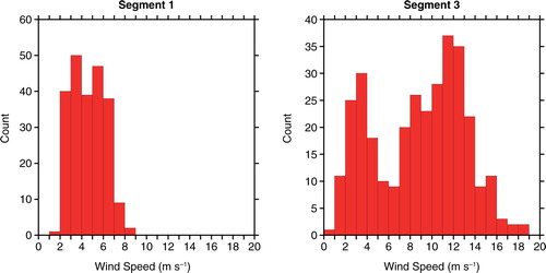
As with data from SO GasEx (Ho et al., 2011b), the parameterisations of Nightingale et al. (2000b), Ho et al. (2006) and Wanninkhof et al. (2009) are most able to model the data from GasEx-98. Wanninkhof (1992) is able to accurately represent the results for segment 1, but not for segment 3. This can be explained by the difference in wind speed distributions between the two segments (Fig. 6). Segment 1 covers a narrow range of wind speeds, from 1.9 to 8.6 m s⁻¹, with a mean (± standard deviation) of 4.6±1.5 m s⁻¹. Segment 3 covers a large range of wind speeds, from 0.9 to 18.3 m s⁻¹ with a mean (± standard deviation) of 8.8±4.2 m s⁻¹ and can be used effectively to distinguish the differences in the various wind speed/gas exchange parameterisations. This result shows one of the advantages of this approach, in that it can distinguish between differences in wind speed/gas exchange relationships due to the differences in distributions of the wind speeds, while other approaches are limited to simply evaluating mean k from mean wind speeds and over fixed time intervals.

Fig. 6 Wind speed distributions of segments 1 and 3 of the ³He/SF₆ data, shows that segment 1 covered a more narrow range of wind speeds than segment 3, with a mean wind speed that was about half of segment 3.

Segment 1 covers a period with decreasing winds, while segment 3 covers a period with increasing winds. One could expect a period with increasing winds to have younger and steeper waves, and greater wave breaking and bubble mediated gas transfer (Kleiss and Melville, 2010). However, the k(600) as a function of wind speed is similar from these two periods, indicating that for these intervals there were no difference between increasing and decreasing winds.

Of note is that over the last week of the study, ³He/SF₆ ratio changes were very small while winds were in the intermediate range 3–10 m s⁻¹ (Fig. 2). This appears in part due to significant mixed layer deepening from 20 to 30 m during this period and diurnal stratification during periods of low winds (Zhang et al., 2001). This observation also suggests that for GasEx-98, residual turbulence due to thermal gradients in the mixed layer and surface shear had little impact on k, in contrast to GasEx-2001 in the equatorial Pacific where CO₂ eddy covariance measurements suggested a significant enhancement (McGillis et al., 2004).

3.6. Similarity between different ocean basins

The results from GasEx-98 show that the relationship between wind speed and gas exchange in the North Atlantic is similar to that of the Southern Ocean. Ho et al. (2011b) showed that in the open ocean, for slightly soluble gases such as CO₂, there appears to be a universal relationship between wind speed and gas exchange as the very similar parameterisations of Nightingale et al. (2000b), Ho et al. (2006) and Wanninkhof et al. (2009) derived from different datasets and assumptions (Fig. 3) are able to account for 82, 83 and 80% of the variance, respectively, in the ³He/SF₆ dual tracer data collected in open and coastal oceans. With the addition of data from GasEx-98, these statistics have not changed significantly, and Nightingale et al. (2000b), Ho et al. (2006) and Wanninkhof et al. (2009) are able to account for 83, 83 and 81% of the variance in all the ³He/SF₆ data, respectively.

3.7. Global constraints

The parameterisations that can explain most of the variance in the ³He/SF₆ during GasEx-98 also match the global constraints based on bomb ¹⁴C. Sweeney et al. (2007) used an ocean general circulation model to reproduce the global bomb ¹⁴C ocean inventory, based on a quadratic dependence between wind speed and gas exchange that has a coefficient very similar to that of Ho et al. (2006) (Table 3). Wanninkhof (2014) revised the analysis performed in Wanninkhof (1992), with updated global wind speed and bomb ¹⁴C inventories, and obtained a relationship that is 30% lower than in the original analysis, is nearly identical to that of Ho et al. (2006), and falls well within the uncertainty of the other parameterisations (Table 3).

Table 3. Wind speed/gas exchange parameterisations that are able to reproduce the ³He/SF₆ results from GasEx-98 and other studies in the coastal and global oceans, and global relationships based on ¹⁴C

Citation	Approach	Region	Parameterisations^a
Nightingale et al. (2000b)	^3He/SF6	North Sea and Georges Bank	^b
Ho et al. (2006)	^3He/SF6	Southern Ocean
Sweeney et al. (2007)	^14C	Global	(±30%)^c
Wanninkhof et al. (2009)	Synthesis	Global
Wanninkhof (2014)	^14C	Global	(±30 %)^c

^aFor all parameterisations, u ₁₀ is in m s⁻¹ while the resulting k is in cm h⁻¹.

^bIn the literature, investigators have chosen to express wind speed/gas exchange parameterisations as either k(600) or k(660), corresponding to Schmidt numbers of 600 (CO₂ in freshwater at 20 °C) or 660 (close to 666, which is CO₂ in seawater at 20 °C), respectively. This choice is arbitrary. The conversion from k(600) to k(660) requires a multiplication of 0.953 assuming the dependence of gas exchange on Schmidt number scales to Sc^−1/2, for example, for Ho et al. (2006), is equivalent to .

^cThe uncertainty in the global ¹⁴C relationships includes both the uncertainty in wind speeds and global bomb ¹⁴C inventory.

4. Conclusions

Reanalysis of the GasEx-98 data show that the relationship between wind speed and gas exchange is similar between the North Atlantic and the Southern Ocean. Furthermore, the results are in agreement with wind speed/gas exchange parameterisations that have previously been deemed to be the most appropriate to use for predicting gas exchange of slightly soluble gases in the ocean.

With our current knowledge, we are able to predict the rate of gas exchange in the open ocean for slightly soluble gases such as CO₂. The agreement between ³He/SF₆ dual tracer studies in different parts of the ocean and agreement with parameterisations that meet the global ¹⁴C constraint suggest that these relationships can be used for estimating fluxes from air–sea concentration differences if no direct flux estimates are available. There are environments such as those affected with strong shear, thermal induced turbulence, partial ice coverage or extreme turbulence (McGillis et al., 2004; McNeil and D'Asaro, 2007; Loose et al., 2014) where the current wind speed/gas exchange parameterisations have limited capabilities and should be investigated. Other topics that remain to be investigated include the influence of surfactant on gas exchange in upwelling areas or in inland seas, and air–sea exchange of soluble gases, such as DMS and CH₃Br, that might not be as heavily influenced by bubbles.

Acknowledgements

We thank the officers and crew of the NOAA Ship Ronald H. Brown for their help during the experiment, J. Edson for providing the wind speed data, P. Schlosser for measuring the ³He samples. Funding for GasEx-98 was provided by the NOAA Global Carbon Cycle program (Grant NA96GP0201). All data used in the analysis here can be found at: <http://www.aoml.noaa.gov/ocd/gcc/gasex98/>.

Notes

To access the supplementary material to this article, please see Supplementary files under ‘Article Tools’.

References

- Broecker W. S. , Peng T.-H. , Östlund G. , Stuiver M . The distribution of bomb radiocarbon in the ocean. J. Geophys. Res. 1985; 99: 6953–6970. DOI: http://dx.doi.org/10.1029/JC090iC04p06953 .
- Fairall C. W. , Bradley E. F. , Rogers D. P. , Edson J. B. , Young G. S . Bulk parameterization of air–sea fluxes for tropical ocean global atmosphere coupled ocean atmosphere response experiment. J. Geophys. Res. 1996; 101: 3747–3764.
- Ho D. T. , Law C. S. , Smith M. J. , Schlosser P. , Harvey M. , co-authors . Measurements of air–sea gas exchange at high wind speeds in the Southern Ocean: implications for global parameterizations. Geophys. Res. Lett. 2006; 33: 16611. DOI: http://dx.doi.org/10.1029/2006GL026817 .
- Ho D. T. , Sabine C. L. , Hebert D. , Ullman D. S. , Wanninkhof R. , co-authors . Southern Ocean Gas Exchange Experiment: setting the stage. J. Geophys. Res. 2011a; 116 C00F08. DOI: http://dx.doi.org/10.1029/2010jc006852 .
- Ho D. T. , Wanninkhof R. , Schlosser P. , Ullman D. S. , Hebert D. , co-authors . Towards a universal relationship between wind speed and gas exchange: gas transfer velocities measured with 3He/SF6 during the Southern Ocean Gas Exchange Experiment. J. Geophy. Res. 2011b; 116: 00F04. C10010, DOI: http://dx.doi.org/10.1029/2010JC006854 .
- Hood E. M. , Wanninkhof R. , Merlivat L . Short timescale variations of fCO2 in a North Atlantic warm-core eddy: results from the Gas-Ex 98 carbon interface ocean atmosphere (CARIOCA) buoy data. J. Geophys. Res. 2001; 106: 2561–2572.
- Kim D. O. , Lee K. , Choi S. D. , Kang H. S. , Zhang J. Z. , co-authors . Determination of diapycnal diffusion rates in the upper thermocline in the North Atlantic Ocean using sulfur hexafluoride. J. Geophys. Res. 2005; 110 C10010. DOI: http://dx.doi.org/10.1029/2004JC002835 .
- Kleiss J. M. , Melville W. K . Observations of Wave breaking kinematics in fetch-limited seas. J. Phys. Oceanogr. 2010; 40: 2575–2604. DOI: http://dx.doi.org/10.1175/2010JPO4383.1 .
- Kuss J. , Nagel K. , Schneider B . Evidence from the Baltic Sea for an enhanced CO2 air–sea transfer velocity. Tellus B. 2004; 56: 175–182. DOI: http://dx.doi.org/10.1111/j.1600-0889.2004.00092.x .
- Law C. S. , Watson A. J. , Liddicoat M. I . Automated vacuum analysis of sulfur hexafluoride in seawater: derivation of the atmospheric trend (1970–1993) and potential as a transient tracer. Marine Chem. 1994; 48: 57–69. DOI: http://dx.doi.org/10.1016/0304-4203(94)90062-0 .
- Liss P. S. , Merlivat L , Buat-Ménard P . Air–sea gas exchange rates: Introduction and synthesis. The Role of Air–Sea Exchange in Geochemical Cycling. 1986. D. Reidel, Dordrecht, pp. 113–127.
- Loose B. , McGillis W. R. , Perovich D. , Zappa C. J. , Schlosser P . A parameter model of gas exchange for the seasonal sea ice zone. Ocean. Sci. 2014; 10: 17–28. DOI: http://dx.doi.org/10.5194/os-10-17-2014 .
- Ludin A. , Weppernig R. , Bönisch G. , Schlosser P . Mass spectrometric measurement of helium isotopes and tritium in water samples. 1998; Palisades, NY: Lamont-Doherty Earth Observatory. pp. 42.
- McGillis W. R. , Edson J. B. , Hare J. E. , Fairall C. W . Direct covariance air–sea CO2 fluxes. J. Geophys. Res. 2001a; 106: 16729–16745. DOI: http://dx.doi.org/10.1029/2000JC000506 .
- McGillis W. R. , Edson J. B. , Ware J. D. , Dacey J. W. H. , Hare J. E. , co-authors . Carbon dioxide flux techniques performed during GasEx-98. Mar. Chem. 2001b; 75: 267–280. DOI: http://dx.doi.org/10.1016/S0304-4203(01)00042-1 .
- McGillis W. R. , Edson J. B. , Zappa C. J. , Ware J. D. , McKenna S. P. , co-authors . Air–sea CO2 exchange in the equatorial Pacific. J. Geophys. Res. 2004; 109: 08S02. DOI: http://dx.doi.org/10.1029/2003JC002256 .
- McNeil C. , D'Asaro E . Parameterization of air–sea gas fluxes at extreme wind speeds. J. Mar. Syst. 2007; 66: 110–121. DOI: http://dx.doi.org/10.1016/j.jmarsys.2006.05.013 .
- Nightingale P. D. , Liss P. S. , Schlosser P . Measurements of air–sea gas transfer during an open ocean algal bloom. Geophys. Res. Lett. 2000a; 27: 2117–2120. DOI: http://dx.doi.org/10.1029/2000GL011541 .
- Nightingale P. D. , Malin G. , Law C. S. , Watson A. J. , Liss P. S. , co-authors . In situ evaluation of air–sea gas exchange parameterizations using novel conservative and volatile tracers. Glob. Biogeochem. Cycle. 2000b; 14: 373–387. DOI: http://dx.doi.org/10.1029/1999GB900091 .
- Peng T. H. , Broecker W. S. , Mathieu G. G. , Li Y. H. , Bainbridge A. E . Radon evasion rates in the Atlantic and Pacific Oceans as determined during the GEOSECS program. J. Geophys. Res. 1979; 84: 2471–2486. DOI: http://dx.doi.org/10.1029/JC084iC05p02471 .
- Salter M. E. , Upstill-Goddard R. C. , Nightingale P. D. , Archer S. D. , Blomquist B. , co-authors . Impact of an artificial surfactant release on air–sea gas fluxes during Deep Ocean Gas Exchange Experiment II. J. Geophys. Res. 2011; 116: 11016. DOI: http://dx.doi.org/10.1029/2011jc007023 .
- Sweeney C. , Gloor E. , Jacobson A. R. , Key R. M. , McKinley G. , co-authors . Constraining global air–sea gas exchange for CO2 with recent bomb C-14 measurements. Glob. Biogeochem. Cycle. 2007; 21: 2015. DOI: http://dx.doi.org/10.1029/2006GB002784 .
- Wanninkhof R . Relationship between gas exchange and wind speed over the ocean. J. Geophys. Res. 1992; 97: 7373–7381. DOI: http://dx.doi.org/10.1029/92JC00188 .
- Wanninkhof R. , Asher W. , Weppernig R. , Chen H. , Schlosser P. , co-authors . Gas transfer experiment on Georges Bank using two volatile deliberate tracers. J. Geophys. Res. 1993; 98: 20237–20248. DOI: http://dx.doi.org/10.1029/93JC01844 .
- Wanninkhof R. , Hitchcock G. , Wiseman B. , Vargo G. , Ortner P. B. , co-authors . Gas exchange, dispersion, and biological productivity on the West Florida Shelf: results from a Lagrangian Tracer Study. Geophys. Res. Lett. 1997; 24: 1767–1770. DOI: http://dx.doi.org/10.1029/97GL01757 .
- Wanninkhof R. , McGillis W. R . A cubic relationship between air–sea CO2 exchange and wind speed. Geophys. Res. Lett. 1999; 26: 1889–1892. DOI: http://dx.doi.org/10.1029/1999GL900363 .
- Wanninkhof R. , Sullivan K. F. , Top Z . Air–sea gas transfer in the Southern Ocean. J. Geophys. Res. 2004; 109: 08S19. DOI: http://dx.doi.org/10.1029/2003JC001767 .
- Wanninkhof R. , Asher W. E. , Ho D. T. , Sweeney C. , McGillis W. R . Advances in Quantifying Air–Sea Gas Exchange and Environmental Forcing. Ann. Rev. Mar. Sci. 2009; 1: 213–244. DOI: http://dx.doi.org/10.1146/annurev.marine.010908.163742 .
- Wanninkhof R . Relationship between wind speed and gas exchange over the ocean revisited. Limnol. Oceanogr. Methods. 2014; 12: 351–362. DOI: http://dx.doi.org/10.4319/lom.2014.12.351 .
- Watson A. J. , Upstill-Goddard R. C. , Liss P. S . Air–sea gas exchange in rough and stormy seas measured by a dual tracer technique. Nature. 1991; 349: 145–147. DOI: http://dx.doi.org/10.1038/349145a0 .
- Zhang J.-Z. , Wanninkhof R. , Lee K . Enhanced new production observed from the diurnal cycle of nitrate in an oligotrophic anticyclonic eddy. Geophys. Res. Lett. 2001; 28: 1579–1582. DOI: http://dx.doi.org/10.1029/2000GL012065 .