Variability and trends of carbon parameters at a time series in the eastern tropical Atlantic

Abstract

Hourly fCO₂ is recorded at a time series at the PIRATA buoy located at 6°S 10°W in the eastern tropical Atlantic since June 2006. This site is located south and west of the seasonal Atlantic cold tongue and is affected by its propagation from June to September. Using an alkalinity–salinity relationship determined for the eastern tropical Atlantic and the observed fCO₂, pH and the inorganic carbon concentration are calculated. The time series is investigated to explore the intraseasonal, seasonal and interannual timescales for these parameters, and to detect any long-term trends. At intraseasonal timescales, fCO₂ and pH are strongly correlated. On seasonal timescales, the correlation still holds between fCO₂ and pH and their variations are in agreement with those of sea surface salinity. At interannual timescales, some important differences appear in 2011–2012: lower fCO₂ and fluxes are observed from September to December 2011 and are explained by higher advection of salty waters at the mooring, in agreement with the wind. In early 2012, the anomaly is still present and associated with lower sea surface temperatures. No significant long-term trend is detected over the period 2006–2013 on CO₂ and any other physical parameter. However, as atmospheric fCO₂ is increasing over time, the outgassing of CO₂ is reduced over the period 2006–2013 as the flux is mainly controlled by the difference of fCO₂ between the ocean and the atmosphere. A longer time series is required to determine if any significant trend exists in this region.

• fugacity of CO₂
• ocean acidification
• time series
• eastern tropical Atlantic

To access the supplementary material to this article, please see Supplementary files under ‘Article Tools’.

1. Introduction

Since the last decades, the continuous increase of global atmospheric CO₂ has led to an increase of CO₂ in the ocean reducing the CO₂ concentration remaining in the atmosphere. However, this continuous absorption of CO₂ has consequences on the chemistry of the ocean and then, on the biology. When CO₂ is absorbed by the ocean, it reacts with seawater to form carbonic acid, which increases ocean acidity by releasing H⁺ ions (and hence decreases the pH of surface waters), increases the inorganic carbon and decreases the concentration of carbonate ions . The decrease of reduces the saturation states of calcium carbonates (calcite and aragonite). This will lead to a shallower saturation horizon which will affect marine organisms that secrete CaCO₃ to produce their shells or skeletons (Orr et al., 2005) and gradually slow down the production of calcium carbonate in the surface ocean (Riebesell et al., 2000).

As the CO₂ concentration in the ocean varies on seasonal and spatial scales, time series are the best means to describe the long-term evolution of biogeochemical properties and changes in interannual variability. The pH can be calculated using two other carbon parameters among the fugacity of CO₂ (fCO₂), inorganic carbon (TCO₂) and alkalinity (TA), when pH is not directly measured. From subpolar to tropical oceanic regions, most of the time series have already shown a decrease of pH and of the saturation state of calcium carbonate (Ω) over time.

In the Iceland Sea, using measurements of pCO₂ and TCO₂ from 1985 to 2008, Olafsson et al. (2009) calculated a pH winter decrease of 0.024 yr⁻¹ over the period 1985–2008 and low values of aragonite saturation state, with a mean of 1.5, that decrease at a rate of 0.0072 yr⁻¹. Most of the decrease is explained by the uptake of anthropogenic CO₂ Olafsson et al. (2009). At high latitudes, the saturation state of aragonite is low, usually less than 2 (e.g. Azetsu-Scott et al., 2010) and undersaturation of aragonite has already occurred in surface water in some regions of the Arctic, such as the south-eastern Hudson Bay (Azetsu-Scott et al., 2014) and the Canadian Arctic archipelago (Chierici and Fransson, 2009).

A decrease of pH and aragonite saturation state was also observed off the south coast of Japan from a time series at 136–140°E over the period 1998–2004 (Ishii et al., 2011). In different regions of the world ocean, a decrease of pH has been reported, for example, in the Atlantic subtropical gyre such as the European Station for Time series in the Ocean at the Canary Islands (ESTOC) and the Bermuda Atlantic Time-series Study (BATS), for periods over 15 years (Bates et al., 2014), at a time series station in the North Pacific near Hawaii over 20 years (Dore et al., 2009).

A trend is more difficult to detect in regions with very high variability. For example, in the southern California system, affected by intermittent upwelling, hourly fCO₂ has been monitored at the Santa Monica Bay Observatory (33°56′N, 118°43′W) from 2003 to 2008 but no trend of pH has been observed in the surface layer (Leinweber and Gruber, 2013). However, pH and the aragonite saturation state decrease below 100 m over the 6-year period.

In the equatorial Pacific, using pCO₂ measurements made at four moorings and the relation of Lee et al. (2006) to calculate alkalinity, Sutton et al. (2014) detected a decreasing pH trend associated with anthropogenic CO₂ absorption but also due to increased upwelling.

In the tropical Atlantic, there is a paucity of time series stations. However, according to Feely and Doney (2009), the tropical Atlantic is expected to experience the most dramatic changes in absolute value of saturation state as it has the highest saturation states of calcium carbonates.

On the western side of the tropical Atlantic, TA and pH have been monitored monthly at the CARIACO site (10°30′N, 64°40′W) on the northern Venezuelan margin, since 1995. A significant increase of fCO₂ over time is observed from 1996 to 2008 and is mainly related to the increase of sea surface temperature (SST) (Astor et al., 2005). The decrease of pH is not statistically significant during that period (p value of 0.25) but a significant pH decrease of −0.0025 yr⁻¹ (p value<0.01) is observed on a longer timescale from 1995 to 2011 (Bates et al., 2014).

On the eastern side of the tropical Atlantic, hourly fCO₂ and yearly TCO₂/TA have been measured at the PIRATA (Prediction and Research moored Array in the Tropical Atlantic, Bourlès et al., 2008) mooring (6°S 10°W) since June 2006 (Lefèvre et al., 2008). Using data from 2006 to 2009, Parard et al. (2010) evidenced the impact of cold water from the upwelling on the fCO₂ distribution at this site. Focusing on the diurnal variability they explained the variability of fCO₂ by biological or thermodynamical processes. They found a net community production ranging from 9 to 41 mmol C·m⁻²·d⁻¹ in agreement with estimates for tropical regions. In this paper, we present observations at this site over the 2006–2013 period. Using fCO₂ measurements recorded at the mooring and alkalinity estimated from sea surface salinity (SSS), we calculate the other variables of the carbon system (pH and TCO₂). After describing the environmental setting (section 3), we analyse the processes affecting the carbon system at this site, on seasonal (section 4.1), intraseasonal and short-term (section 4.2) and interannual variability (section 4.3). Finally, we examine the trends of pH, fCO₂ and physical parameters over the period 2006–2013 in section 4.4.

2. Material and methods

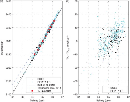
A CO₂ CARIOCA sensor has been installed on the mooring at 6°S 10°W to monitor hourly fCO₂ in the surface layer (1.5 m). The time series started in June 2006. The hourly distributions of fCO₂ and SST are recorded from June 2006 to October 2013. The distribution of SSS is hourly until April 2012 and is available on a daily basis only, after April 2012. After April 2012, all calculations are made on a daily basis. The accuracy of the fCO₂ measurements using this spectrophotometric method with thymol blue is estimated at±3 µatm (Hood and Merlivat, 2001). The sensor is calibrated at the Division Technique (Institut National des Sciences de l'Univers, France) before and after deployment with a CO₂ system including a Licor 7000. In 2006 and 2011, the sensors recorded data until a new sensor replaced them in 2007 and 2012, respectively. The values measured by the new sensor matched the last values of the old sensor. For the other years, the sensors stopped measuring before the time of their replacement due to electronic failures. Possible drifts (increase of fCO₂) due to biofouling could occur. In order to assess such a drift, we use the oxygen concentration measured at the mooring with an Anderaa optode to detect biofouling. The oxygen concentrations exhibit large diurnal cycles when biofouling occurs (see Fig. 1 in Lefèvre and Merlivat, 2012). In this case, the data are disregarded. The PIRATA mooring is also equipped with temperature and salinity sensors in the water column (at depths 1.50, 20, 40, and 120 m), and atmospheric instruments (rain gauge, anemometer, atmospheric pressure sensor, air temperature and humidity sensors) (2008). Once a year, during the cruise for servicing the mooring, seawater samples are taken for TCO₂ and TA measurements. The samples are analysed using potentiometric titration derived from the method developed by Edmond (1970) with a closed cell. The calculations of the equivalent points are estimated using a non-linear regression method (DOE, 1994). For calibration, Certified Reference Materials (CRMs) provided by Prof. A. Dickson (Scripps Institution of Oceanography, San Diego, USA) are used. From 2005 to 2007, during the AMMA program (Redelsperger et al., 2006), two cruises per year were realised. The accuracy is estimated at±3 µmol/kg for both TCO₂ and TA. Measurements collected from 2005 to 2007 during the EGEE cruises in the eastern tropical Atlantic have been used to determine an alkalinity–salinity relationship for the region 10°S–6°N 10°W–10°E (Koffi et al., 2010) with a standard error on predicted alkalinity of±7.2 µmol/kg:1 Recent TA measurements made from 2009 to 2015 during the PIRATA France (PIRATA FR) cruises confirm that this relationship is still valid (Fig. 1). We have calculated the 10-quantiles that divide the dataset into 10 subsets of equal size. The 10-quantiles are indicated on Fig. 1a (red squares) and follow the relationship of Koffi et al. (2010) even for low and high SSS values. In addition, the comparison of the relationship with the relationships of Takahashi et al. (2014) (Fig. 1a) and of Lee et al. (2006) (Fig. 1b) shows that the Koffi et al.'s relationship is really the most suitable for the region. Surface seawater pH, and TCO₂ are then calculated from estimated TA and measured fCO₂ at the mooring. Seawater pH is calculated on the total scale at the SST. The program CO2sys of Pierrot et al. (2006) is used for the calculations. To remove the effects of precipitation/evaporation, TCO₂ is normalised to a mean SSS of 36 (nTCO₂=36*TCO₂/SSS).

Fig. 1 (a) Alkalinity–salinity relationships of Koffi et al. (2010) and Takahashi et al. (2014). The dots correspond to the 190 data used (EGEE cruises from 2005 to 2007) for determining the Koffi et al.'s relationship and the crosses correspond to the 349 new data collected during the PIRATA FR cruises from 2009 to 2015. The 10-quantiles are indicated in red. (b) Differences between the observations and the alkalinity calculated with the relationship of Lee et al. (2006) as a function of salinity.

According to Lauvset and Gruber (2014), when pH is not measured, the best pair of the carbon system to calculate pH is fCO₂ and TA, even with TA estimated from SSS.

Daily fluxes of CO₂ are calculated using the daily SST, SSS and wind speed measured at the mooring and the gas exchange coefficient (k) of Sweeney et al. (2007) and the solubility (So) of Weiss (1974):2

As atmospheric CO₂ (fCO_{2 atm}) is not measured at the mooring, we use the monthly molar fraction of CO₂ (xCO_{2 atm}) recorded at the atmospheric station at Ascension Island (7.92°S, 14.42°W) of the NOAA/ESRL Global Monitoring Division (www.esrl.noaa.gov/gmd/ccgg/iadv/). At this location, the atmospheric fCO₂ has increased at a rate of 2.0 µatm yr⁻¹ over the period 2006–2013. The atmospheric pressure was taken from the NCEP/NCAR (National Centers for Environmental Prediction/National Center for Atmospheric Research) reanalysis project (Kalnay et al., 1996) as some data gaps exist at the mooring.

A monthly CO₂ climatology has been constructed at 6°S 10°W by taking the mean of the overall months over the period June 2006–October 2013. The anomalies are defined as the differences between the monthly observations and the climatological monthly value. Although there are large data gaps in the time series, this approach removes most of the seasonal variability and allows the detection of trends as reported by Bates et al. (2014).

Anomalies of physical parameters (wind, temperature, salinity) are defined in the same way and are differences between monthly observations and monthly climatological means.

The meridional salinity advection is calculated using the second term of the equation of the horizontal salinity advection:3 where u and v are the zonal and meridional components of the ocean current and S is the salinity. The monthly means of salinity and ocean currents for the period from 2006 to 2013 are obtained from the new Mercator Ocean (Toulouse, France) GLORYS2V3 global ocean reanalysis, at 1/4 degree horizontal resolution, with 75 vertical levels, forced by ERA-Interim atmospheric variables and, covering the 1993–2013 time period. This salinity field is only used for the calculation of advection.

The Global Precipitation Climatology Project (GPCP) (Adler et al., 2003; Xie et al., 2003) is used to characterise the precipitation field over the region (resolution 2.5°) and to compare with the data recorded at the mooring.

The SST distribution is examined with the GLORYS2v3 monthly means. The climatological ocean circulation is examined by using the OSCAR currents (Bonjean and Lagerloef, 2002) available at www.oscar.noaa.gov. Monthly climatological maps of surface currents and of SSTs are constructed for the 2006–2013 period to illustrate the mean seasonal evolution of the surroundings of the mooring at 6°S 10°W.

3. Hydrological variability

The mooring is located in the eastern equatorial Atlantic (EEA), a region characterised by an important seasonal cycle that affects SST, SSS and surface currents. The most important signal is in the SST with the formation of the Atlantic cold tongue (ACT). Its setup is well correlated with the increase of the south-easterlies and the northward migration of the InterTropical Convergence Zone (ITCZ) (Picaut, 1983). This cooling appears every year from May–June to October and affects a band south of the Equator, from the African coast to 20°W. The cooling is of the order of 5–7 °C during the cold season from May to October (mean SSTs from 23 to 26 °C) while from November to April SSTs rise from 26 to 29 °C (Merle, 1980).

SSS values are higher than 36 and much lower in the eastern part of the EEA. The lowest values (<33) occur along the African coast due to river outflow, that is, the Niger and Congo rivers (Da-Allada et al., 2014). The seasonal variability of SSS depends on the seasonal variability of river runoff, precipitation and also on the intensity and direction of the main surface currents, which modulates the westward transport of low salinity waters (Camara et al., 2015).

The surface current system is composed of two main zonal currents (e.g. Stramma and Schott, 1999): (1) the Guinea Current (GC) that flows eastward north of 2°N; (2) the South Equatorial Current (SEC), located south of 2°N, that flows westward from the African to the South American coast. The SEC can be divided into three branches: the northern, central and southern SEC (Molinari, 1982). The mooring at 6°S 10°W is mainly affected by the central branch of the SEC (cSEC). The opposite SEC and the intense Eastward Undercurrent (EUC) underneath generate vertical shear and intense mixing at the base of the mixed layer. This process is the main source of cooling for the ACT (Foltz et al., 2003; Wade et al., 2011; Giordani et al., 2013; Schlundt et al., 2014).

In January (Fig. 2a), SSTs are the coldest (24 °C) at 12°S and increase to the north, where the highest values are observed north of the equator. During this period, the SEC is barely present. April (Fig. 2b) is the warmest month (SSTs from 27 to 29 °C) over most of the basin. The GC appears more clearly north of 2°S and the SEC has a more defined zonal component. The mooring receives mainly waters from the east and/or north as the meridional component of the surface current is predominantly negative.

Fig. 2 Climatological surface velocity currents superimposed on the SST field for (a) January, (b) April, (c) July and (d) October. The climatology is calculated over the period January 2006–December 2013. The black circle indicates the position of the mooring. The surface velocity currents are from OSCAR and the SST climatology from GLORYS2v3 on a grid of 0.25° resolution.

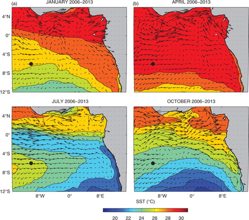
In July (Fig. 2c), the ACT is observed from the African coast to at least 12°W and from 4°S to the equator. The ACT is limited to the north by the Equatorial SST Front which separates the cold waters of the ACT (<22 °C) from the warmer equatorial waters (>25 °C) of the GG. The mooring is located south of the ACT, in waters of about 25 °C. During this period, the SEC is well developed and occupies the area between 8°S and 3°N, while the GC is restricted to a coastal band of the GG.

In October (Fig. 2d), the coldest SSTs are observed south of the region, close to the mooring. The zonal component of the SEC has considerably decreased while the GC has a strong eastward component which turns southward near the coast of Africa. North of 4°S, surface warming occurs with SSTs reaching 28 °C in the GG.

4. Results and discussions

4.1. Seasonal variability of the mooring data

SST, SSS, fCO₂ variations are plotted for each year of the period 2006–2013 (Fig. 3), in order to characterise the different scales of variability, from intraseasonal to interannual. The difference of fCO₂ between the ocean and the atmosphere (ΔfCO₂) and CO₂ fluxes are presented at daily scale for the whole time series on Fig. 4. Monthly variations of SST, SSS and fCO₂ are computed as box and whisker plot to highlight their seasonal variations and spread (Fig. 5). Moreover, mean seasonal values of monthly climatological SST, SSS, TCO₂, nTCO₂, pH and TA are gathered in Table 1, as well as correlations between monthly values in Table 2.

Fig. 3 Hourly distribution of (a) SST, (b) SSS and (c) fCO₂ from January to December for the years 2006 to 2013. From April 2012 the high resolution SSS is not available so mean daily data are plotted. Orange shaded areas correspond to high fCO₂ associated with low SST (see text for details).

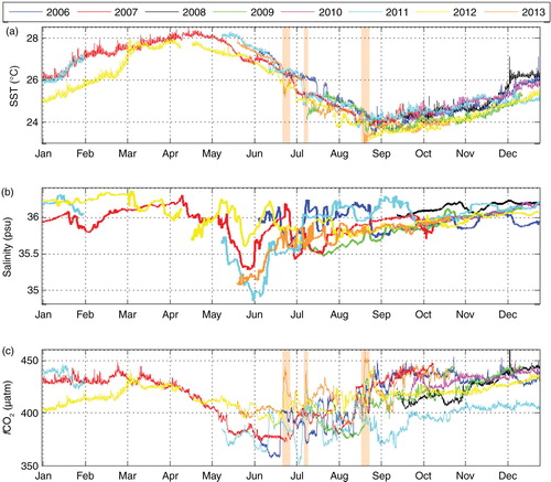
Fig. 4 (a) Daily difference of fCO₂ between the ocean and the atmosphere (ΔfCO₂) and (b) daily CO₂ fluxes over the whole time series.

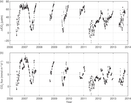
Fig. 5 Box and whisker plots of daily (a) SST, (b) SSS and (c) fCO₂ for each month of the time series. The horizontal red line corresponds to the median, the blue box to the data between the first and third quartiles, the error bars to the minimum and maximum, and the crosses to outliers. The black line corresponds to the monthly climatology 2006–2013.

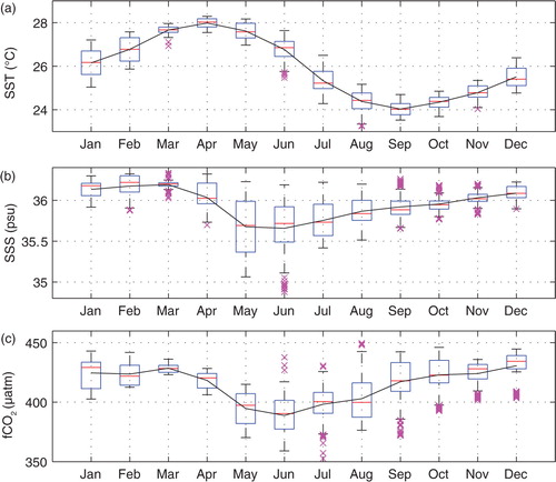
Table 1. Seasonal values of monthly climatological SST, SSS, fCO₂, pH, TCO₂, nTCO₂ and TA calculated over 2006–2013 at 6°S, 10°W: minimum, maximum, range, mean, standard deviation (STD), median and interquartile range (IQR)

	SST (°C)	SSS (psu)	fCO2 (µatm)	pH	TCO2 ( µmol·kg^−1)	nTCO2 (µmol·kg^−1)	TA (µmol·kg^−1)
Min	23.98	35.67	388	8.022	2007	2022	2340
Max	27.86	36.19	431	8.055	2063	2066	2374
Range	3.87	0.52	43	0.033	56	43	34
Mean	25.87	35.96	414	8.035	2044	2046	2359
STD	1.40	0.18	15	0.0116	20	15	2
Median	25.72	35.98	421	8.029	2050	2047	2360
IQR	2.63	0.31	24.17	0.019	29	25.57	20

Table 2. Correlation between monthly variables calculated over the period 2006–2013

	SST (°C)	SSS (psu)	fCO2 (µatm)	pH	TCO2 (µmol·kg^−1)	nTCO2 (µmol·kg^−1)
SST	1	0.13	−0.13	0.06	−0.59	−0.90
SSS		1	0.92	−0.93	0.71	0.28
fCO2			1	−0.997	0.86	0.54
pH				1	−0.82	−0.48
TCO2					1	0.87
nTCO2						1

The correlations are statistically significant (p value<0.05 level) except those in italic.

The seasonal cycle of SST is quite regular (Fig. 3a), while, in contrast, the SSS and fCO₂ distributions show significant variability mainly during the cold season (Fig. 3b and c). Warm and salty waters are observed from January to April (warm season) and have high fCO₂ values greater than 400 µatm. From May, both SST and SSS are decreasing and explain the fCO₂ decrease at the beginning of the cold season. The minimum of fCO₂ in June corresponds to a minimum of SSS more or less pronounced depending on the year (Fig. 3b). At this time of the year the westward advection of Congo and Niger waters explains the freshening of the ACT until mid-June (Schlundt et al., 2014). The location of the mooring, between the salty southern waters and the ACT region, explains the high fCO₂ variability with values that could vary 20–30 µatm over a few days period (Fig. 3c). From November, the variability becomes smaller and fCO₂ reaches values over 400 µatm.

The daily ΔfCO₂ over the whole time series show positive values except in June 2006 with a slight undersaturation of −8 µatm and in July 2011 when the undersaturation reaches −25 µatm (Fig. 4a). The CO₂ fluxes follow the same pattern as the fCO₂ distribution with minimum values in June while CO₂ outgassing is dominating the region (Fig. 4b). The wind speed is relatively stable (between 5 and 8 m/s) as the region is dominated by the southeasterly trade winds. Therefore, the CO₂ flux is mainly influenced by the difference of fCO₂ between the ocean and the atmosphere. On monthly average, the CO₂ flux varies between 0.51 mmol·m⁻²·d⁻¹ in September 2011 and a maximum of 11.56 mmol·m⁻²·d⁻¹ in January 2007.

The monthly climatology of SST has a regular pattern (Fig. 5a) with seasonal variations of 4 °C, a maximum of 27.86 °C in April and a minimum of 23.98 °C in September (Table 1). SSS and fCO₂ show a large range (resp. 0.5 and 43 µatm) with their minimum values occurring during the cold season, in June and higher outside the ACT period (Fig. 5b and c and Table 1). The interquartile range (IQR) is also presented to show the variability of the dataset. It is defined as the difference between the third quartile and the first quartile and measures how spread the 50 % of the dataset is. The largest IQR are observed from May to August for both variables (Fig. 5b and c), that is, during the ACT period. A high correlation (0.92) exists between SSS and fCO₂, while the correlation between fCO₂ and SST is weak and statistically non-significant (Table 2). At a seasonal timescale, the lack of correlation between fCO₂ and SST can be explained by two opposed effects: the seasonal cooling in the ACT favours fCO₂ decrease, but as the cooling in the ACT is mainly a consequence of mixing between mixed layer and upper thermocline waters, high fCO₂ are brought up from the subsurface thus leading to an fCO₂ increase.

Compared to the Atlantic time series presented by Bates et al. (2014), PIRATA has the highest fCO₂ (lowest pH) with CARIACO. The pH calculated hourly varies from 8.012 to 8.068 (Table 1). The climatological pH values are within the range observed in the western tropical Atlantic at the CARIACO station, where pH and alkalinity are measured monthly (Astor et al., 2005), but exhibit a smaller seasonal variation consistent with the smaller variation also observed on fCO₂. As CARIACO is located in a coastal upwelling region, the seasonal range of fCO₂ is larger with a value of 58±17 µatm (Astor et al., 2013) compared to our value of 43 µatm. In the productive costal upwelling, fCO₂ can decrease significantly below the atmospheric value whereas the values at 6°S 10°W rarely go below the atmospheric level. At 6°S 10°W, the monthly climatological fCO₂ and pH are strongly anti-correlated (Table 2) as the pH distribution is the mirror of the fCO₂ distribution. Because of this tight correlation between fCO₂ and pH, the factors affecting the variability of fCO₂ will also explain the variability of pH. Note that pH is highly anti-correlated to SSS variations while no significant correlation is observed with SST (Table 2). Compared to the open ocean time series stations ESTOC and BATS, in the subtropical gyre, the PIRATA site exhibits higher SSS seasonal variation (>0.5) but similar fCO₂ variability as ESTOC (Santana-Casiano et al., 2007), whereas at BATS the fCO₂ variability can reach 80 µatm (Bates et al., 2014).

The mean values of TCO₂ (2044±20 µmol·kg⁻¹) and TA (2359±12 µmol·kg⁻¹) at 6°S 10°W are lower than at the CARIACO site (2072±26 µmol·kg⁻¹ and 2413±19 µmol·kg⁻¹, respectively) and at ESTOC (TCO₂=2096±6 µmol·kg⁻¹, TA>2400 µmol·kg⁻¹, Santana-Casiano et al., 2007). The much lower alkalinity at 6°S 10°W explains the higher mean fCO₂ of 414±15 µatm compared to 395±22 µatm at CARIACO. The normalisation of TCO₂ to the mean SSS of 36 reduces the TCO₂ variability by only 23 % with nTCO₂ exhibiting seasonal variations over 40 µmol·kg⁻¹ (Table 1). The correlation of TCO₂ with SSS is smaller and TCO₂ is explained by both SSS and SST (Table 2). The anti-correlation between TCO₂ and SST suggests a carbon supply by the CO₂-rich ACT, a feature observed in upwelling regions. When the SSS effect on TCO₂ is minimised by the normalisation to a constant SSS, the correlation with SST becomes stronger (Table 2). The upwelling-like effect would lead to a negative fCO₂–SST relationship but the warming of the water would lead to a positive fCO₂–SST relationship. Both processes are at play here, which would explain the lack of correlation between fCO₂ (pH) and SST.

4.2. Short-term and intraseasonal variability at the mooring

The high frequency sampling at 6°S 10°W reveals significant short-term variations on fCO₂, SSS, SST and on daily CO₂ fluxes (Fig. 3). The diurnal variability observed on temperature and fCO₂ has already been addressed by Parard et al. (2010) who attributed diurnal variations to thermodynamic or biological processes at the mooring. Using the daily changes of TCO₂, they calculated a net community production (NPP) integrated over the mixed layer, ranging from 9 to 41 mmol C·m⁻²·d⁻¹, in agreement with estimates of NPP for tropical regions.

Because of its location close to the mid-Atlantic ridge, the mooring is influenced by internal waves generated by the submarine topography. Internal waves promote the development of biological activity and supply nutrients into the mixed layer, leading to a rapid decrease of TCO₂ in the surface layers (Parard et al., 2014).

Here we focus on a bit longer timescale when strong fluctuations of fCO₂ are generated from 2 days to 2 weeks. The strongest intraseasonal variability is observed during the cold season from May to October, whereas short-term variations are rather small during the warm season (November–April) (see Fig. 3 and also IQR in Fig. 4). The ACT, which results for the incorporation of subsurface waters into the mixed layer mainly by vertical turbulent mixing, is colder and richer in CO₂ than the surrounding water. During this period, the fCO₂ and SST distributions exhibit strong variations within a few days. This is particularly visible in 2013 (orange curve in Fig. 3) with clear intrusions of low SST and high fCO₂ values (orange shaded area in Fig. 3a and c) associated with the proximity of the ACT. For instance, the SST decreases from 26.5 to 25.15 °C in only 2 days, 25–27 June (Fig. 3a). This signal is clearly associated with an increase of fCO₂ from 400 to 444 µatm (Fig. 3c). Another peak of fCO₂ of the same magnitude is observed on the 12–13 July associated with an SST decrease of about 0.8 °C. A larger peak is observed on the 23–24 August 2013 with an increase of fCO₂ close to 60 µatm associated with a decrease of SST of 1.5 °C.

All these rapid and high fluctuations of both SST and fCO₂ suggest that horizontal rather than vertical processes are active. The ACT is not present at the mooring during this period because it is located further north. However, on its southern boundary, a wave activity is present (Marin et al., 2009; Giordani and Caniaux, 2014), not as intense as in the equatorial front in its northern boundary, but still able to generate filaments and vortices. These mesoscale features can detach from the ACT and migrate to the south, with cooling and increase of fCO₂ through horizontal advection at the mooring (see Fig. 2 of Parard et al., 2010).

4.3. Interannual variability

During the cold season, the variability of CO₂ in the vicinity of the mooring strongly depends on the position of the ACT that displays significant year to year variability (Caniaux et al., 2011). With the proximity of the ACT, CO₂-rich waters associated with relatively cold temperature are observed at the mooring. However, this effect is more or less pronounced depending on the year. Correlations between fCO₂ and SST, TCO₂ and SST are given for July to September each year (Supplementary Table 1). Outside the cold season, there is weak or no correlation.

Although the year to year variability of fCO₂ is expected to be mainly caused by the year to year variability of the ACT, the fCO₂ record at 6°S 10°W shows a significant difference from September 2011 to early 2012. In September 2011, low fCO₂ values are observed and remain significantly low until April 2012, compared to other years (Fig. 3a). Parameters recorded at the mooring such as precipitation and zonal wind, negative for westward, and meridional wind, positive for northward (Fig. 6) are now examined to investigate the anomaly. Monthly values are used in order to detect noticeable features that could impact the fCO₂, SSS and SST distributions. The mooring is located in a region where the surface water budget is dominated by evaporation. Almost no precipitation is recorded throughout the year except some rain events occurring in April 2008, May 2009 and April 2011 (Fig. 6a). Unfortunately, only the impact of the rain events of 2011 can be seen on fCO₂, as fCO₂ measurements are missing in 2008 and 2009 at the time of the other rain events. In 2011, the maximum of precipitation in April is followed by a minimum of SSS in June (Fig. 3b). The minimum of SSS is accompanied by a decrease of fCO₂ in June (Fig. 3c). After this event, fCO₂ remains low until July, before increasing around 400 µatm in October with the increase of SSS (Fig. 3c). Apart from the rain events, the variability of SSS is not caused by local precipitation. As a matter of fact, the SSS decreases by more than 0.6 in May 2007 and yet no noticeable precipitation is recorded at the mooring that year. Thus, another factor may be responsible for the SSS decrease at that time of the year at the location of the buoy. Certainly, horizontal advection plays a strong role during this period as suggested by Berger et al. (2014). Each year in May–June, SSS decreases to reach its minimum value (Fig. 3b) when the surface layer starts cooling and the cSEC intensifies. This low salinity is accompanied by decrease of fCO₂. However, the intensity of the SSS decrease varies from one year to another with a stronger decrease in 2011 and a less pronounced decrease in 2012 (cyan and yellow curves in Fig. 3b).

Fig. 6 Monthly distribution of (a) precipitation, (b) zonal wind and (c) meridional wind at the mooring. The precipitation from GPCP is represented in red and the precipitation at the PIRATA mooring in blue. The black line corresponds to the monthly climatology calculated over 2006–2013. The mean of the zonal and meridional wind components is −4.70 and 4.29 m/s, respectively. The zonal and meridional components of the wind are blue shaded with their respective 2006–2014 mean used as the base level. A zonal negative wind corresponds to a wind blowing westward and a positive meridional wind corresponds to a wind blowing northward. (d) Zonal wind anomaly and (e) meridional wind anomaly from 2006 to 2013.

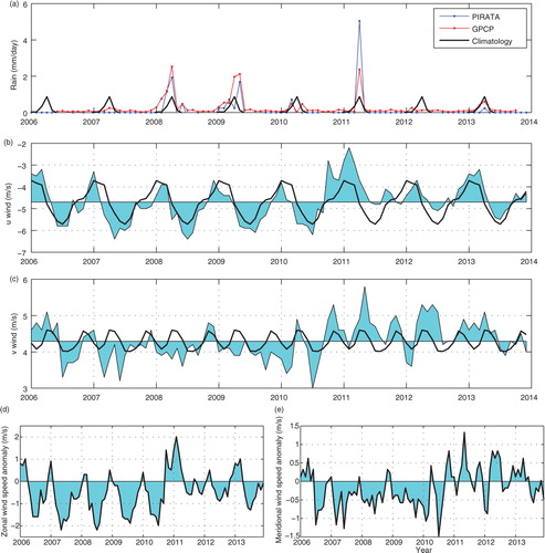
Another specific feature of 2011 is the weak zonal wind with an absolute value that remains below 5 m/s throughout the year (Fig. 6b). It is accompanied by an increase of the meridional component of the wind (Fig. 6c). Moreover, 2011 is characterised by the lowest annual zonal wind (absolute value of 4.0 m/s) and the highest meridional wind (4.7 m/s) over the 2006–2013 period, two features appearing clearly on the zonal (Fig. 6d) and meridional wind anomalies (Fig. 6e). As the zonal component weakens and the meridional components strengthens, surface water coming from the south of the mooring location may be advected and reach the site.

The ACT is characterised by fresh and CO₂-rich waters whereas the waters further south are more saline and closer to the CO₂ equilibrium. This is confirmed by transects performed along the line 10°S–20°S, around 15°W, during the months of July and December: near-equilibrium conditions were sampled whereas higher values were observed in April–June due to higher SST (Lefèvre et al., 1998). The region is also characterised by high SSS. At the PIRATA mooring located at 10°S, 10°W, SSS is usually higher than 36 throughout the year (Berger et al., 2014).

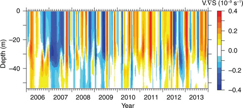
In order to confirm intrusions of salty water from the south, salinity advection is calculated from the MERCATOR PSY2V4R2 model, for each of the 19 near surface levels (from the surface to 53 m depth) in the box area 9°S–6°S 9.5°W–10.5°W. Monthly salinity advection anomalies are calculated by removing monthly data climatology. The meridional salinity advection anomalies confirm the intrusion of saltier waters south of the mooring, which is particularly pronounced in 2011 (Fig. 7), from the surface down to 40 m depth, and especially from May to July.

Fig. 7 Hovmöller diagram of the meridional salinity anomaly advection (in s⁻¹), averaged over the box 9°S–6°S and 10.5°W–9.5°W, from the surface to 50 m depth.

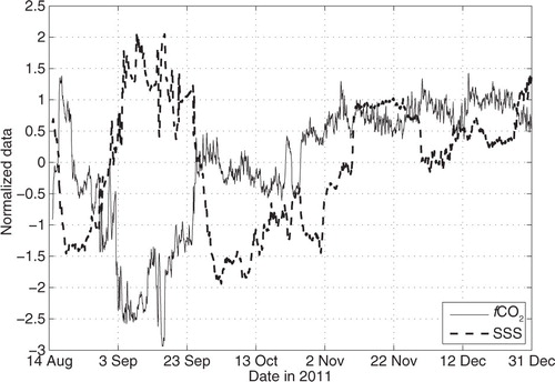
In order to highlight the variations of both fCO₂ and SSS, and to plot the data on the same scale, we normalise them by subtracting the mean of the dataset and dividing the difference by the standard deviation. The distributions of normalised fCO₂ and normalised SSS anomalies show that fCO₂ decreases (increases) are associated with SSS increases (decreases) after mid-August (Fig. 8), a pattern still observed until the end of the year 2011 although it becomes weaker from November. A strong fCO₂–SSS anti-correlation is obtained for the period 14 August 2011–2 November 2011 (r ²=0.70).

Fig. 8 Normalised fCO₂ ((fCO₂ – <fCO₂>)/σ _fCO2 ) and normalised SSS ((SSS – <SSS>)/σ_SSS) data at 6°S, 10°W from 14 August 2011 to 31 December 2011.

From September to December 2011, the fCO₂ variability is mainly driven by the SSS variations whereas, from December 2011 to May 2012, there is clear signal on the SST. From the end of 2011, the SST decreases and remains lower, until May 2012, in comparison with other years (see Fig. 3a). As a result, fCO₂ is also lower.

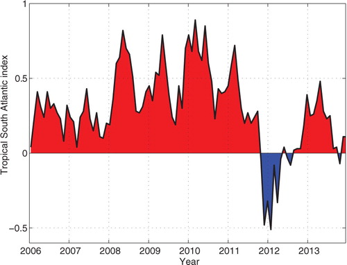
These low SSTs observed at the mooring from December 2011 to March 2012 correspond to a much larger cooling that affected an extended part of the South Atlantic basin. This is evidenced by considering the variability of the Tropical South Atlantic (TSA) index calculated as the mean SST in the region 30°W–10°E 20°S–0° (Enfield et al., 1999) (Fig. 9). The TSA has cooled down substantially since December 2011 to March 2012 probably due to an intensification of the southeasterly trade winds. A similar feature was reported for 2012 in the tropical Pacific by England et al. (2014). Consequently, the low seawater fCO₂ values observed in 2011–2012 lead to a reduced outgassing (Fig. 3d). From June 2006 to October 2007 the CO₂ outgassing is 6.83±3.44 mmol·m⁻²·d⁻¹ whereas for the same period in 2011–2012 the flux is reduced by about half with an outgassing of 3.37±2.27 mmol·m⁻²·d⁻¹.

Fig. 9 Tropical South Atlantic index from 2006 to 2013. The index is calculated as the area-averaged monthly SST anomalies over the region 30°W–10°E, 20°S–0°. The anomalies are deviations from the 1951–2000 climatology (www.esrl.noaa.gov/psd).

4.4. Long-term trends

In order to examine the trends of the carbon parameters fCO₂, pH and TCO₂ over time, the monthly climatology 2006–2013 is removed and the anomalies are plotted as a function of time (Fig. 10a–c). There is substantial variability on a year to year basis but no trend in carbon parameters is detected over the period 2006–2013. The regressions with the statistics are presented in Supplementary Table 2. As a longer record is available for SST and SSS, we examine the anomalies at the mooring over the period 2000–2014 (Fig. 10d and e). However, in the period 2006–2014, the SST time series presents a significant break-point in 2012 that can be detected by applying the statistical non-parametric test of Pettitt (1979). This means that considering the whole segment 2006–2014 for calculating the trend of the series is not appropriate. Over this period, the chronological SST series presents a significant negative trend of −0.151 °C/month (blue line in Fig. 10d), which does not reflect the behaviour of the whole series. For this reason, we prefer computing the tendency over the period 2006–2011. Over this segment, the slope of the regression is positive (green line) but not significant at the 0.05 level. For the series beginning in 2000 (red line in Fig. 10d), a weak positive trend is also detected but again the test is not significant at the 95 % confidence level. This means that, since 2000 or for the period 2006–2011, SSTs at the buoy did not experience any significant tendency.

Fig. 10 Time series of (a) fCO₂, (b) pH, (c) TCO₂ anomalies over the period 2006–2013 with regression line (green). (d) Time series of SST anomalies over the period 2000–2014. Solid lines correspond to the linear regressions for the periods 2000–2014 (red, SST=0.00516*time – 10.36352), 2006–2012 (green, SST=−0.0056*time+11.39793), 2006–2014 (blue) where time is in years; dashed lines correspond to the 95 % confidence intervals of the regressions over the various time segments, (e) time series of SSS anomalies over the period 2000–2014. Solid lines correspond to the linear regressions for the periods 2000–2014 (red, SSS=0.00575*time – 11.53567) and 2006–2014 (blue, SSS=0.00685*time – 13.75012); dashed lines correspond to the 95 % confidence intervals of the regressions over both time segments.

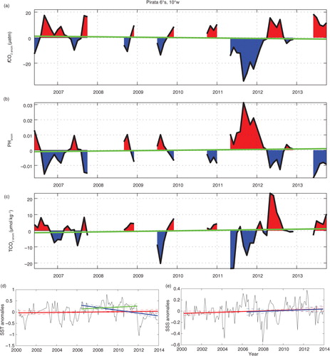
The SSS linear regression presents weak positive slopes (red and blue lines, respectively, Fig. 10e) but both are non-significant at the 95 % confidence level. Again, we conclude that no significant trend affects SSS at the PIRATA buoy like for SSTs.

The strong correlation between pH and fCO₂ observed at seasonal scale (−0.997, Table 2) is maintained for the non-seasonal variability but there is also a tight link with nTCO₂ (−0.995, Supplementary Table 3). On the other side, no strong correlations exist between the SST and SSS anomalies and the carbon parameters anomalies (Supplementary Table 3). The highest correlation is between TCO₂ and SSS (0.61) but the correlation between fCO₂ and SSS, strong at seasonal scale (0.92, Table 2), is not significant at non-seasonal timescales (−0.22, Supplementary Table 3).

The lack of any trend of SST and SSS could contribute to the difficulty in detecting a trend of fCO₂. At the CARIACO site, the fCO₂ time series presents a trend of 1.77±0.43 µatm/yr (from 1996 to 2008) that is mainly explained by the SST increasing at a rate of 0.09±0.02 °C/yr. When the temperature effect is removed, the rate of increase of fCO₂ becomes 0.51±0.49 µatm/yr and is not significant (Astor et al., 2013). Using the carbon system equations, we can calculate that a decrease in SSS with no other changes would lead to a decrease of pH. An increase of SST would also decrease the pH. In the subtropical gyres, the increase of fCO₂ is close to the one observed at CARIACO with a rate of 1.69±0.11 µatm/yr at BATS (from 1983 to 2012) and 1.92±0.24 µatm/yr at ESTOC (from 1996 to 2012). The pH decrease is statistically significant at these stations with −0.0017±0.0001 unit/year (BATS) and −0.0018±0002 unit/year (ESTOC).

At 6°S 10°W water masses from different origin (from the northern ACT or from south of 6°S) arrive to the mooring so that measurements over a longer period does not reflect the presence of the same water mass and explain the large year to year variability observed at this site. Using 10 Earth system models, Bopp et al. (2013) estimate a global sea surface reduction of pH ranging from −0.07 to −0.33 pH unit for the 2090s compared to 1990s. They also predict a low acidification rate for the tropical Atlantic. At the mooring, the seasonal variability of pH is about 0.03, which suggests that the ecosystem there is probably adapted to large pH variations.

As the CO₂ flux decreases over time during 2006–2013, we calculated the anomalies to confirm the trend. Both the CO₂ flux and ΔfCO₂ decrease over time but no significant trend is detected on seawater fCO₂ and wind speed. The decrease of ΔfCO₂ is explained by the increase of atmospheric fCO₂ over that period. As the CO₂ flux shows the same pattern as ΔfCO₂ and is weakly related to the wind speed, a decrease of the CO₂ flux is observed during that period. However, the strong 2011–2012 anomaly near the end of the record and the strong flux observed in 2006–2007 could bias the trend, meaning that a longer record would be necessary to confirm the existence of any trend.

It is interesting to note that Goyet et al. (1998) did not detect any change of seawater fCO₂ when comparing the WOCE A15 data with the FOCAL cruise made 10 years earlier (Andrié et al., 1986) but the continuous increase of atmospheric fCO₂ led them to conclude to a weaker source of CO₂ along 19°W. The same mechanism is observed here. On the other hand, Oudot et al. (1995) came to the opposite conclusion after observing an increase of fCO₂ in 1993 compared to the FOCAL cruises at 4°W and 35°W in the equatorial Atlantic. At the CARIACO site, a stronger rate of seawater fCO₂ increase has been detected from 1995 to 2011 compared to 1996–2008, which suggests a stronger outgassing in recent year (Bates et al., 2014). Using different methodologies to estimate the seasonal, interannual variability and trends of the CO₂ flux in the Atlantic, Schuster et al. (2013) concluded to a steady source of the tropical Atlantic from 1995 to 2009 although different methods disagree and the region suffers from a lack of measurements.

5. Conclusions

Hourly measurements of fCO₂ have been made since June 2006 at the mooring at 6°S 10°W. This time series has been used to analyse the intraseasonal, seasonal and interannual timescales which affect the carbon parameters. As an alkalinity–salinity relationship is available specifically for this region, the carbon parameters (pH and TCO₂) can be calculated from fCO₂ and alkalinity. As fCO₂ and pH are closely related, the variability of fCO₂ explains the pH variability at this site. The mooring is located in the EEA where the variability is dominated by the seasonal formation of the ACT. During the cold season (May–October), mesoscale features detach from the ACT, generate cooling and increase fCO₂ at the mooring through horizontal advection, which mostly explains the intraseasonal variability on fCO₂, particularly pronounced during the cold season.

On seasonal timescale, fCO₂ and pH are strongly correlated with SSS whereas no correlation is observed with SST. During the cold season, fCO₂ and TCO₂ are negatively correlated with SST exhibiting an upwelling-type behaviour although the site is located south of the ACT region. A strong interannual variability has been detected over the period 2006–2013 with intrusions of southern and saltier waters in 2011–2012 compared to the other years. The impact of cooling of the South Atlantic from December 2011 to March 2012 is visible at 6°S 10°W with lower SST and fCO₂. This interannual anomaly is responsible for a lower CO₂ outgassing at the mooring in 2011–2012. As the cooling of 2011–2012 extends to a large region, it is likely that such interannual event affects the air–sea CO₂ flux on a larger scale.

Over the 7 years of the time series at 6°S 10°W, no significant trend can be detected in fCO₂, pH and TCO₂ in the surface layer. The data period is still short and the gaps in the record due to technical failures make it difficult to determine a trend. However, even the SST and SSS do not present any trend over a longer period (2000–2013) and on a record without data gaps. This is in contrast with the western tropical Atlantic, where an increase of fCO₂ over time is detected at the CARIACO site and is mostly explained by the trend on SST (Astor et al., 2013). Detecting a trend in fCO₂ and pH at 6°S 10°W is impeded by the complex ocean circulation that causes high variability in the carbon parameters. Over the period 2006–2014 no ocean acidification is detected.

Long-term sustained observations are necessary to better document the processes affecting this region given the strong variability at this site. In addition, more CO₂ sensors would be required to monitor the carbon properties in other parts of the tropical Atlantic and help to better understand the evolution of the source of CO₂ at the basin scale.

6. Acknowledgements

We acknowledge support from the European Integrated Projects CARBOOCEAN (contract 511176-2) and CARBOCHANGE (grant agreement 264879), the Institut de Recherche pour le Développement (IRD) and the national program LEFE CYBER. We are very grateful to US IMAGO of IRD, and especially to Jacques Grelet and Fabrice Roubaud for their technical support at sea and the deployment of the sensor. We thank the DT INSU for preparation and calibration of the CARIOCA sensor. Seawater samples were analysed for TCO₂ and TA by the SNAPO-CO₂ at LOCEAN in Paris. Data management for PIRATA moorings is conducted by the TAO project office at NOAA/PMEL in collaboration with many research institutes listed on the PIRATA website (www.pmelnoaa.gov/pirata). Precipitation data from the GPCP were downloaded from the Giovanni online data system, developed and maintained by the NASA Goddard Earth Sciences (GES) Data and Information Services Center (DISC). We also acknowledge the TRMM mission scientists and associated NASA personnel for production of the data used in this research effort. TMI data are produced by Remote Sensing Systems and sponsored by the NASA Earth Science and REASoN DISCOVER project. They are available at www.remss.com. We thank Fabrice Hernandez from IRD for making available to us the products of the Mercator Ocean (Toulouse, France) GLORYS2V3 global ocean reanalysis. We acknowledge the OSCAR Project Office for providing the ocean surface current analyses. The fCO₂ data at 6°S 10°W presented here are publicly available at the Carbon Dioxide Information and Analysis Center (CDIAC), www.cdiac.ornl.gov/oceans/ and in the SOCAT database (www.socat.info). We are grateful to Rik Wanninkhof and an anonymous reviewer for their comments that improve the manuscript.

Notes

To access the supplementary material to this article, please see Supplementary files under ‘Article Tools’.

References

- Adler R. F. , Huffman G. J. , Chang A. , Ferraro R. , Xie P.-P. , co-authors . The version 2 Global Precipitation Climatology Project (GPCP) monthly precipitation analysis (1979–Present). J. Hydrometeor. 2003; 4: 1147–1167.
- Andrié C. , Oudot C. , Genthon C. , Merlivat L . CO2 fluxes in the tropical Atlantic during FOCAL cruises. J. Geophys. Res. 1986; 91(C10): 11741–11755.
- Astor Y. M. , Scranton M. I. , Muller-Karger F. E. , Bohrer R. , Garcia J . fCO2 variability at the CARIACO tropical coastal upwelling time series station. Mar. Chem. 2005; 97(3–4): 245–261.
- Astor Y. M. , Lorenzoni L. , Thunell R. , Varela R. , Muller-Karger F. , co-authors . Interannual variability in sea surface temperature and fCO2 changes in the CARIACO basin. Deep-Sea Res. II. 93 , 33–43. 2013. http://dx.doi.org/10.1016/j.dsr1012.2013.1001.1002 .
- Azetsu-Scott K. , Starr M. , Mei Z.-P. , Granskog M . Low calcium carbonate saturation state in an arctic inland sea having large and varying fluvial inputs: the Hudson Bay system. J. Geophys. Res. 2014; 119: 6210–6220. http://dx.doi.org/6210.1002/2014JC009948 .
- Azetsu-Scott K. , Clarke A. , Falkner K. , Hamilton J. , Jones E. P. , co-authors . Calcium carbonate saturation states in the waters of the Canadian Arctic Archipelago and the Labrador Sea. J. Geophys. Res. 2010; 115: 11021. http://dx.doi.org/10.1029/2009JC005917 .
- Bates N. , Astor Y. M. , Church M. J. , Currie K. , Dore J. E. , co-authors . A time-series view of changing ocean chemistry due to ocean uptake of anthropogenic CO2 and acidification. Oceanography. 2014; 27(1): 126–141. http://dx.doi.org/110.5670/oceanog.2014.5616 .
- Berger H. , Treguier A.-M. , Perenne N. , Talandier C . Dynamical contribution to sea surface salinity variations in the eastern Gulf of Guinea based on numerical modelling. Clim. Dyn. 2014; 43: 3105–3122. http://dx.doi.org/3110.1007/s00382-00014-02195-00384 .
- Bonjean F. , Lagerloef G. S. E . Diagnostic model and analysis of the surface currents in the tropical Pacific Ocean. J. Phys. Oceanogr. 2002; 32(10): 2938–2954.
- Bopp L. , Resplandy L. , Orr J. C. , Doney S. C. , Dunne J. P. , co-authors . Multiple stressors of ocean ecosystems in the 21st century: projections with CMIP5 models. Biogeosciences. 2013; 10: 6225–6245. http://dx.doi.org/6210.5194/bg-6210-6225-2013 .
- Bourlès B. , Lumpkin R. , McPhaden M. J. , Hernandez F. , Nobre P. , co-authors . The PIRATA program: history, accomplishments, and future directions. Bull. Am. Meteorol. Soc. 2008; 89: 1111–1125.
- Camara I. N. , Kolodziejczyk N. , Mignot J. , Lazar A . On the seasonal variations of salinity of the tropical Atlantic mixed layer. J. Geophys. Res. 2015; 120: 4441–4462. http://dx.doi.org/4410.1002/2015JC010865 .
- Caniaux G. , Giordani H. , Redelsperger J.-L. , Guichard F. , Key E. , co-authors . Coupling between the Atlantic cold tongue and the West African monsoon in boreal spring and summer. J. Geophys. Res. 2011; 116: 04003. http://dx.doi.org/10.1029/2010JC006570 .
- Da-Allada Y. C. , Alory G. , DuPenhoat Y. , Jouanno J. , Hounkonnou M. N. , co-authors . Causes for the recent increase in sea surface salinity in the north-eastern Gulf of Guinea. African. Afr. J. Mar. Sci. 2014; 36(2): 197–205.
- Chierici M. , Fransson A . Calcium carbonate saturation in the surface water of the Arctic Ocean: undersaturation in freshwater influenced shelves. Biogeosciences. 2009; 6: 2421–2432.
- DOE. Handbook of methods for the analysis of the various parameters of the carbon dioxide system in sea water, ORNL/CDIAC-74. 1994; Oak Ridge, TN. pp. 1–30: DOE. eds A.G. Dickson & C. Goyet). Determination of total alkalinity in seawater.
- Dore J. E. , Lukas R. , Sadler D. W. , Church M. J. , Karl D. M . Physical and biogeochemical modulation of ocean acidification in the central North Pacific. Proc. Natl. Acad. Sci. USA. 2009; 106(30): 12235–12240. http://dx.doi.org/12210.11073/pnas.0906044106 .
- Edmond J. M . High precision determination of titration alkalinity and total carbon dioxide content of seawater by potentiometric titration. Deep Sea Res. 1970; 17(4): 737–750.
- Enfield D. B. , Mestas A. M. , Mayer D. A. , Cid-Serrano L . How ubiquitous is the dipole relationship in tropical Atlantic sea surface temperatures?. J. Geophys. Res. 1999; 104: 7841–7848.
- Feely R. A. , Doney S. C . Ocean acidification present and future. Oceanography. 2009; 22(4): 36–47.
- Foltz G. R. , Grodsky S. A. , Carton J. A. , McPhaden M. J . Seasonal mixed layer heat budget of the tropical Atlantic Ocean. J. Geophys. Res. 2003; 108(C5): http://dx.doi.org/10.1029/2002JC001584 .
- Giordani H. , Caniaux G . Lagrangian Sources of frontegenesis in the equatorial Atlantic front. Clim. Dyn. 2014. 43 (TACE special issue), 3147–3162. DOI: http://dx.doi.org/10.1007/s00382-014-2293-3 .
- Giordani H. , Caniaux G. , Voldoire A . Intraseasonal mixed-layer heat budget in the equatorial Atlantic during the cold tongue development in 2006. J. Geophys. Res. 2013; 118(2): 650–671.
- Goyet C. , Adams R. , Eischeid G . Observations of the CO2 system properties in the tropical Atlantic Ocean. Mar. Chem. 1998; 60(1–2): 49–61.
- Hood E. M. , Merlivat L . Annual to interannual variations of fCO2 in the northwestern Mediterranean Sea: results from hourly measurements made by CARIOCA buoys, 1995–1997. J. Mar. Res. 2001; 59(1): 113–131.
- Ishii M. , Kosugi N. , Sasano D. , Saito S. , Midorikawa T. , co-authors . Ocean acidification off the south coast of Japan: a result from time series observations of CO2 parameters from 1994 to 2008. J. Geophys. Res. 2011; 116: 06022. http://dx.doi.org/10.1029/2010JC006831 .
- Kalnay E. , Kanamitsu M. , Kistler R. , Collins W. , Deaven D. , co-authors . The NCEP/NCAR 40-year reanalysis project. Bull. Am. Meteorol. Soc. 1996; 77(3): 437–471.
- Koffi U. , Lefèvre N. , Kouadio G. , Boutin J . Surface CO2 parameters and air–sea CO2 flux distribution in the eastern equatorial Atlantic Ocean. J. Mar. Syst. 2010; 82: 135–144.
- Lauvset S. K. , Gruber N . Long-term trends in surface ocean pH in the North Atlantic. Mar. Chem. 2014; 162: 71–76.
- Lee K. , Tong L. T. , Millero F. J. , Sabine C. , Dickson A. G. , co-authors . Global relationships of total alkalinity with salinity and temperature in surface waters of the world's oceans. Geophys. Res. Lett. 2006; 33: 19605. http://dx.doi.org/10.1029/2006GL027207 .
- Lefèvre N. , Guillot A. , Beaumont L. , Danguy T . Variability of fCO2 in the Eastern Tropical Atlantic from a moored buoy. J. Geophys. Res. 2008; 113 C01015. DOI: http://dx.doi.org/10.1029/2007JC004146 .
- Lefèvre N. , Merlivat L . Carbon and oxygen net community production in the eastern tropical Atlantic estimated from a moored buoy. Global Biogeochem. Cycles. 2012; 26: 1009. http://dx.doi.org/10.1029/2010GB004018 .
- Lefèvre N. , Moore G. , Aiken J. , Watson A. , Cooper D. , co-authors . Variability of pCO2 in the tropical Atlantic in 1995. J. Geophys. Res. 1998; 103(C3): 5623–5634.
- Leinweber A. , Gruber N . Variability and trends of ocean acidification in the Southern California current system: a time series from Santa Monica Bay. J. Geophys. Res. 2013; 118: 3622–3633. http://dx.doi.org/3610.1002/jgrc.20259 .
- Marin F. , Caniaux G. , Bourlès B. , Giordani H. , Gouriou Y. , co-authors . Why were sea surface temperature conditions so different in the eastern equatorial Atlantic in June 2005 and 2006. J. Phys. Oceanogr. 2009; 39: 1416–1431. http://dx.doi.org/10.1175/2008JPO4030.1 .
- Merle J . Variabilité thermique annuelle et interannuelle de l'océan Atlantique équatorial Est. L'hypothèse d'un “El Niño” Atlantique. Oceanologica Acta. 1980; 3(2): 209–220.
- Molinari R. L . Observations of eastward currents in the tropical South Atlantic Ocean: 1978–1980. J. Geophys. Res. 1982; 87(C12): 9707–9714.
- Olafsson J. , Olafsdottir S. R. , Benoit-Cattin A. , Danielsen M. , Arnason T. S. , co-authors . Rate of Iceland Sea acidification from time series measurements. Biogeosciences. 2009; 6: 2661–2668.
- Orr J. C. , Fabry V. J. , Aumont O. , Bopp L. , Doney S. C. , co-authors . Anthropogenic ocean acidification over the twenty-first century and its impact on calcifying organisms. Nature. 2005; 437(7059): 681–686.
- Oudot C. , Ternon J. F. , Lecomte J . Measurements of atmospheric and oceanic CO2 in the tropical Atlantic: 10 years after the 1982–1984 FOCAL cruises. Tellus B. 1995; 47B: 70–85.
- Parard G. , Lefèvre N. , Boutin J . Sea water fugacity of CO2 at the PIRATA mooring at 6°S, 10°W. Tellus B. 2010; 62(5): 636–648. DOI: http://dx.doi.org/10.1111/j.1600-0889.2010.00503.x .
- Parard G. , Boutin J. , Cuypers Y. , Bouruet-Aubertot P. , Caniaux G . On the physical and biogeochemical processes driving the high frequency variability of CO2 fugacity at 6oS, 10oW: Potential role of the internal waves. J. Geophys. Res. 2014; 119: 8357–8374. http://dx.doi.org/8310.1002/2014JC009965 .
- Pettitt A. N . A non-parametric approach to the change-point problem. Appl. Statist. 1979; 28(2): 126–135.
- Picaut J . Propagation of the seasonal upwelling in the Eastern Equatorial Atlantic. J. Phys. Oceanogr. 1983; 13: 18–37.
- Pierrot D. , Lewis E. , Wallace D. W. R . O. R. N. L . MS excel program developed for CO2 system calculations. Carbon Dioxide Information Analysis Center. 2006; Oak Ridge, TN: U.S. Department of Energy.
- Redelsperger J.-L. , Thorncroft C. D. , Diedhiou A. , Lebel T. , Parker D. J. , co-authors . African monsoon multidisciplinary analysis: an international project and field campaign. Bull. Am. Meteorol. Soc. 2006; 87 1739–1746. DOI: http://dx.doi.org/10.1175/BAMS-1187-1112-1739 .
- Riebesell U. , Zondervan I. , Rost B. , Tortell P. D. , Zeebe R. E. , co-authors . Reduced calcification of marine plankton in response to increased atmospheric CO2 . Nature. 2000; 407: 364–367.
- Santana-Casiano J. M. , Gonzalez Davila M. , Rueda M. J. , Llinas O. , Gonzalez Davila E.-F . The interannual variability of oceanic CO2 parameters in the northeast Atlantic subtropical gyre at the ESTOC site. Global Biogeochem. Cycles. 2007; 21 1–16. DOI: http://dx.doi.org/10.1029/2006GB002788 .
- Schlundt M. , Brandt P. , Dengler M. , Hummels R. , Fischer T. , co-authors . Mixed layer heat and salinity budgets during the onset of the 2011 Atlantic cold tongue. J. Geophys. Res. 2014; 119 7882–7910. DOI: http://dx.doi.org/10.1002/2014JC010021 .
- Schuster U. , McKinley G. A. , Bates N. , Chevallier F. , Doney S. C. , co-authors . . An assessment of the Atlantic and Arctic sea–air CO2 fluxes, 1990–2009. Biogeosciences. 2013; 10: 607–627.
- Stramma L. , Schott F . The mean flow field of the tropical Atlantic Ocean. Deep Sea Res. II. 1999; 46: 279–303.
- Sutton A. J. , Feely R. A. , Sabine C. L. , McPhaden M. J. , Takahashi T. , co-authors . Natural variability and anthropogenic change in equatorial Pacific surface ocean pCO2 and pH. Global Biogeochem. Cycles. 2014; 28: 131–145. http://dx.doi.org/110.1002/2013GB004679 .
- Sweeney C. , Gloor E. , Jacobson A. R. , Key R. M. , McKinley G. , co-authors . Constraining global air-sea gas exchange for CO2 with recent bomb 14C measurements. Global Biogeochem. Cycles. 2007; 21 1–10. DOI: http://dx.doi.org/10.1029/2006GB002784 .
- Takahashi T. , Sutherland S. C. , Chipman D. W. , Goddard J. G. , Ho C. , co-authors . Climatological distributions of pH, pCO2, total CO2, alkalinity and CaCO3 saturation in the global surface ocean, and temporal changes at selected locations. Mar. Chem. 2014; 164: 95–125.
- Wade M. , Caniaux G. , DuPenhoat Y . Variability of the mixed layer heat budget in the eastern equatorial Atlantic during 2005–2007 as inferred using Argo floats. J. Geophys. Res. 2011; 116: 08006. http://dx.doi.org/10.1029/2010JC006683 .
- Weiss R. F . CO2 in water and seawater: the solubility of a non-ideal gas. Mar. Chem. 1974; 2: 203–215.
- Xie P. , Janoviak J. E. , Arkin P. A. , Adler R. F. , Gruber A. , co-authors . GPCP pentad precipitation analyses: an experimental dataset based on gauge observations and satellite estimates. J. Clim. 2003; 16: 2197–2214.