Radon as a tracer of atmospheric influences on traffic-related air pollution in a small inland city

Abstract

One year of radon, benzene and carbon monoxide (CO) concentrations were analysed to characterise the combined influences of variations in traffic density and meteorological conditions on urban air quality in Bern, Switzerland. A recently developed radon-based stability categorisation technique was adapted to account for seasonal changes in day length and reduction in the local radon flux due to snow/ice cover and high soil moisture. Diurnal pollutant cycles were shown to result from an interplay between variations in surface emissions (traffic density), the depth of the nocturnal atmospheric mixing layer (dilution) and local horizontal advection of cleaner air from outside the central urban/industrial area of this small compact inland city. Substantial seasonal differences in the timing and duration of peak pollutant concentrations in the diurnal cycle were attributable to changes in day length and the switching to/from daylight-savings time in relation to traffic patterns. In summer, average peak benzene concentrations (0.62 ppb) occurred in the morning and remained above 0.5 ppb for 2 hours, whereas in winter average peak concentrations (0.85 ppb) occurred in the evening and remained above 0.5 ppb for 9 hours. Under stable conditions in winter, average peak benzene concentrations (1.1 ppb) were 120% higher than for well-mixed conditions (0.5 ppb). By comparison, summertime peak benzene concentrations increased by 53% from well-mixed (0.45 ppb) to stable nocturnal conditions (0.7 ppb). An idealised box model incorporating a simple advection term was used to derive a nocturnal mixing length scale based on radon, and then inverted to simulate diurnal benzene and CO emission variations at the city centre. This method effectively removes the influences of local horizontal advection and stability-related vertical dilution from the emissions signal, enabling a direct comparison with hourly traffic density. With the advection term calibrated appropriately, excellent results were obtained, with high regression coefficients in spring and summer for both benzene (r² ~0.90–0.96) and CO (r² ~0.88–0.98) in the two highest stability categories. Weaker regressions in winter likely indicate additional contributions from combustion sources unrelated to vehicular emissions. Average vehicular emissions during daylight hours were estimated to be around 0.503 (542) kg km⁻² h⁻¹ for benzene (CO) in the Bern city centre.

• radon
• air quality
• urban
• atmospheric stability
• traffic density
• vehicle emissions

1. Introduction

Traffic congestion, and associated emissions (e.g. fine particles, SO₂, NO_x, CO and various hydrocarbons including benzene), is a rapidly growing concern for air quality management in many major urban centres (e.g. Ghose et al., 2004; Chattopadhyay et al., 2007; Sharma and John, 2010; Gulia et al., 2015; Miranda et al., 2015). For benzene and carbon monoxide (CO) pollution in particular, passenger vehicles (cars and motorbikes) are the dominant urban sources (e.g. Verma et al., 2003; Borgie et al., 2014; Hien et al., 2014; Sood et al., 2014; Kim et al., 2015b; Li et al., 2015), although other sources of these pollutants can be significant in industrial or semi-rural settings (e.g. Byrd et al., 1990; ATSDR, 2007; Fan et al., 2014; Borgie et al., 2014; Kim et al., 2015a and references therein).

Urban benzene originates predominantly from the combustion or evaporation of petrol (e.g. Verma and Rana, 2001), whilst CO is primarily a product of incomplete combustion, leading to particularly high emissions at times of heavy traffic congestion when engines are idling and the efficiency of catalytic converters decreases to less than 10% (Sood et al., 2014; Kim et al., 2015b).

Elevated benzene concentrations in urban settings are a concern due to its carcinogenic properties (e.g. Maltoni et al., 2007; Borgie et al., 2014), whereas elevated levels of CO have been linked to a variety of mental health and metabolic issues, and – in some cases – death (Beatty and Shimshack, 2014; Sood et al., 2014; Kim et al., 2015a, 2015b). Consequently, ambient air quality standards devised by regulatory authorities impose thresholds on hourly/daily/yearly mean concentrations of these pollutants to which commuters and residents are exposed. For example, Directive 2000/69/EC of the European Parliament specifies a limit of 5 µg m⁻³ as an annual average for benzene, and 10 mg m⁻³ for CO as a maximum daily mean (EC, 2000; as discussed in Miranda et al., 2015). Switzerland, however, is not part of the EU and has the philosophy that for carcinogenic substances no limit value should be set, as for these compounds concentrations should be kept as small as possible. Effective policing of such guidelines relies upon accurate, widespread monitoring programs, while the planning of timely and effective mitigation strategies depends upon the reliability of regional chemical transport models and the development of accurate regional pollution inventories.

Thermally stable atmospheric conditions and their associated shallow mixing depths are renowned for impeding the dispersion of urban pollution (e.g. Duenas et al., 1996; Perrino et al., 2008; Belušić et al., 2015; Grundstrom et al., 2015; Chambers et al., 2015a). They are also very problematic conditions for numerical models to accurately simulate, in large part due to limitations in model vertical resolution and the ability of parameterisations to accurately represent near-surface mixing processes (e.g. Holtslag, 2014; Koffi et al., 2016). Improved characterisation of near-surface meteorological conditions and their impact on pollutant variability under stable atmospheric conditions is therefore essential in order to improve understanding and representations of physical mixing processes and the associated levels of public exposure during extreme pollution events.

Of the methods presently available to categorise the state of atmospheric stability (Pasquill and Smith, 1983; Perrino et al., 2001; Foken, 2006; Williams et al., 2013; Chambers et al., 2015a), here we employ near-surface measurements of the naturally occurring, radioactive atmospheric tracer Radon-222 (e.g. Chambers et al., 2015a, 2015b). To a good approximation, radon is emitted solely from ice-free, water-unsaturated land surfaces, and its only atmospheric sink is radioactive decay. Radon's half-lifetime (3.82 d) is long enough for it to be considered a conservative tracer over the course of a single night, yet short enough that it does not accumulate in the atmosphere on timescales of more than two weeks. It is also a noble gas, and poorly soluble in water, minimising washout by rain. Finally, radon's surface source function can be considered to be essentially random and uncorrelated with atmospheric processes operating on short temporal (e.g. Holford et al., 1993) and small spatial (e.g. Karstens et al., 2015) scales, so that averaging can be used effectively as a means of isolating effects of interest. For local mixing studies at most inland locations (i.e. away from abrupt geographical changes), variations in the radon surface flux can be neglected on both diurnal timescales and spatial scales comparable to that of a large city. All these characteristics together make radon an ideal tracer for quantifying near-surface atmospheric transport and mixing processes in urban environments (e.g. Perrino et al., 2001; Chambers et al., 2011; Williams et al., 2013).

The aim of this paper is to demonstrate the multiple uses of radon as a tracer to explain observed diurnal characteristics of air pollution levels in a small inland European city (Bern, Switzerland), and to separate the individual influences of: local emissions within the city area; vertical dilution by boundary layer mixing; and horizontal advection of cleaner air from outside the city. This will be accomplished by: (i) characterising the temporal variability in traffic density, radon, benzene and CO emissions at Bern city centre on diurnal and seasonal timescales; (ii) adapting the radon-based stability technique developed by Chambers et al. (2015a) to make it independent of seasonal changes in day length and radon source function; (iii) characterising the combined influence of traffic density and meteorological conditions on benzene and CO concentrations in Bern; and (iv) seeking an accurate relationship between traffic density and pollutant emissions by utilising diurnal radon measurements to remove the effects of local horizontal advection and dilution by atmospheric mixing in this small compact inland city.

2. Methods

2.1. Site and observations

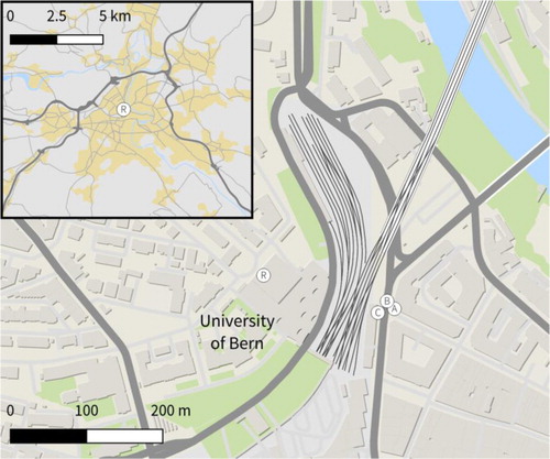
Bern, Switzerland (46° 56′ N, 7° 26′ E; 540 m above sea level), has a population density of approximately 2500 inhabitants km⁻² and is located on the north western foothills of the European Alps. In January 2011, the National Air Pollution Monitoring Network of Switzerland (NABEL; www.bafu.admin.ch/luft/00612/00625/index.html?lang=en) enhanced their existing urban road-curb monitoring site by adding volatile organic carbon monitoring capabilities to a site near the University of Bern (Fig. 1) where routine hourly climatological observations are also made, including air temperature, wind speed and wind direction at 36 m above ground level (a.g.l.). Of the available suite of urban emissions data, this study will focus on CO and benzene as significant traffic-emitted pollutants associated with health impacts. Benzene and CO are sampled from an inlet approximately 3 m above street level.

Fig. 1 Close-up of Bern town centre, showing the location of the radon (R), pollution (A), traffic (B) and meteorological (C) monitoring stations. Small inset shows the location of the measurements within the broader Bern city area. Black lines are railway lines (electric). Map data were obtained from OpenStreetMap (www.openstreetmap.org) and enhanced with Corine Land Cover information (Bosard et al., 2000).

The continuous in-situ CO measurements are made using Cross Flow Modulated Non-Dispersive Infrared Absorption (NDIR; Horiba APMA-360, Kyoto, Japan). Sample gas and reference gas are injected alternately (1 Hz frequency) into the measurement cell using solenoid valve modulation. Sample air is taken to generate CO-free reference gas by using a catalyst to oxidise CO to CO₂. Since the same gas is used for both the sample gas and the reference gas, zero drifts and interference effects are minimised. The detection limit (zero±3σ of the zero signal) is about 30 ppb. The overall measurement uncertainty for a 10 min mean value is estimated to be <10% below 100 ppb and <5% above 100 ppb.

Benzene is analysed using a gas chromatograph (Synspec 955), where every 20 min benzene from 175 ml of ambient air is adsorbed on Tenax GR at room temperature and desorbed at 280 °C. Chromatographic separation is achieved by a BGB 2.5 analytical column (BGB, Adliswil, Switzerland) and detection is performed using a photoionization detector (PID) with a detection limit of 10 ppt.

Traffic density information supplied by NABEL provides the number of vehicles per hour crossing the measurement point on Bollwerkstrasse, a main road through the Bern city centre (Fig. 1).

In addition to the urban curb-side monitoring, continuous direct hourly atmospheric radon concentration measurements were made 150 m away on the roof of the Physics Institute of the University of Bern, using a 700 L dual-flow-loop two-filter radon detector (e.g. Whittlestone and Zahorowski, 1998; Chambers et al., 2014). Sampling was conducted at approximately 45 L min⁻¹ from a height of 15 m a.g.l. A 400 L delay volume was incorporated into the inlet line to ensure virtually all ambient thoron (²²⁰Rn; t_0.5=56 s) was removed from the sampled air stream. The detector has a response time (time to half-peak magnitude) of 45 min, which was partially accounted for in post processing by the removal of a constant 1 hour time lag, and a ‘lower limit of determination’ (radon concentration at which the error for an hourly count reaches 30%) of about 40 mBq m⁻³. The detector was calibrated monthly by injecting radon for 5 hours at ~80 cc min⁻¹ from a 19.19±4% kBq-²²⁶Ra source (PYLON Electronics, http://pylonelectronics.com/). Instrumental background checks were performed every three months.

The period of observations used for this study covers 1 January 2011 to 31 January 2012. All reported times are in local standard time (LST=UTC+1 h), and the northern hemisphere seasonal convention is adopted. No STP corrections have been applied to any of the atmospheric constituent concentrations.

2.2. Radon-based atmospheric stability classification

Near-surface concentrations of urban emissions are closely linked to the atmospheric volume (mixing depth) into which they are mixed (Duenas et al., 1996; Perrino et al., 2001; Chambers et al., 2015a). A proxy frequently used for relative changes in mixing depth is the ‘atmospheric stability’, for which numerous measures based on in-situ meteorological measurements are available, varying considerably in sophistication and ease of application (e.g. Pasquill, 1961; Turner, 1964; Pasquill and Smith, 1983; Foken, 2006).

An alternative to the meteorological methods commonly used for assessing atmospheric stability involves continuous monitoring of near-surface (i.e. ≤20 m a.g.l.) concentrations of the ubiquitous surface-emitted passive tracer radon (e.g. Allegrini et al., 1994; Duenas et al., 1996; Perrino, 2001, 2012; Avino et al., 2003; Galmarini, 2006; Sesana et al., 2006; Chambers et al., 2011, 2015a, 2015b, 2016; Wang et al., 2013; Williams et al., 2013; Kondo et al., 2014; Pitari et al., 2014; Omori and Nagahama, 2016). Radon-derived measures of atmospheric stability, based on accumulation/dilution patterns of radon near the surface, are rapidly gaining acceptance because they are better suited to the analysis of mixing-related changes in nocturnal urban air pollution concentrations than the more traditional techniques based on climatological or turbulence measurements. For example, the radon method works best at precisely those times when Monin-Obukhov classification based on (expensive and labour intensive) eddy correlation measurements fails (i.e. on still, clear nights when turbulence levels are very low and turbulent fluxes are close to zero; Williams et al., 2013). On the other hand, gradient techniques such as those based on forms of the Richardson Number rely on the availability of accurate thermodynamic profiles, and furthermore require careful corrections for the effects of flow distortion by nearby obstacles, mesoscale motions such as nocturnal drainage flows, and intermittent turbulence (e.g. Williams et al., 2013). Finally, the studies by Chambers et al. (2015a, 2015b, 2016) conclusively demonstrate the superiority of the radon-based stability classification over the commonly used measures of Pasquill-Gifford ‘turbulence’ or ‘radiation’ schemes. Radon-based techniques are suited to nocturnal pollution studies because atmospheric radon concentrations near the surface are directly and unambiguously related to the integrated outcome of the turbulent mixing process over a relatively large local footprint, and are comparatively unaffected by site-specific variations in surface flow (roughness) and heating patterns (Williams et al., 2013; Chambers et al., 2015a, 2016). Furthermore, the radon-based stability measures used here can be easily adjusted to suit the regional climatology (Chambers et al., 2015b).

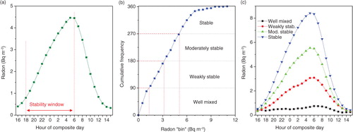
For the present study, we adapt the radon-based stability classification scheme described by Chambers et al. (2015a, 2015b). Application of the original technique involved: (i) splitting the hourly Bern radon time series into fetch-related (large-scale transport) and mixing-related (local diurnal) components by subtracting an hourly time series constructed by interpolating between the afternoon minima; (ii) defining a 12-hour stability window within the diurnal composite (e.g. Fig. 2a); (iii) calculating the cumulative frequency histogram of the window-mean mixing-related radon component; and (iv) using the histogram quartile ranges to define atmospheric stability classes (e.g. Fig. 2b). These stability classes were subsequently used to categorise near-surface observations of atmospheric constituents (e.g. Fig. 2c).

Fig. 2 (a) Diurnal composite of the diurnal-only component of the entire 13-month Bern radon time series; (b) cumulative frequency histogram of mean radon concentrations within the 12-hour ‘stability window’ each night, with quartile ranges indicated; and (c) diurnal composite near-surface radon concentrations corresponding to four atmospheric stability categories defined using the quartiles.

Upon comparing seasonal characteristics of nocturnal radon accumulation under stable conditions (Fig. 3a), however, it became evident that the change in day length between summer and winter results in a significantly longer accumulation time for radon in winter. To accommodate this variability within the radon-based stability classification scheme, it was found to be sufficient to reference the nocturnal accumulation curve each night to the 1900 h radon concentration, and to change to using a 10-hour (1900–0500 h) stability window (e.g. Fig. 3b) to match the accumulation time of the shortest night of the year.

Fig. 3 (a) Diurnal composites of the diurnal-only component of Bern radon concentrations in summer and winter; and (b) seasonal radon accumulation curves at Bern referenced to the 1900 h radon concentration.

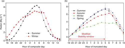
Looking at Fig. 3b, an additional seasonal influence on the Bern radon concentrations now becomes apparent. The rate of diurnal radon accumulation under stable conditions reduces significantly in winter compared to summer and spring. This occurs despite strong evidence from our traffic and pollutant data (discussed in Section 3.3), and also from other studies in this region (e.g. Collaud Coen et al., 2014), that nocturnal mixing depths are on average smaller in winter than in summer, which would result in a tendency towards increased radon accumulation. We therefore conclude that there is a significant reduction in the local/regional radon source function in winter, probably due to snow cover, high soil moisture or partially frozen soils. Larson (1974) estimated that snow cover on soils that were not saturated prior to freezing reduces the radon flux by 20–40%. Monthly mean radon fluxes for the Bern region, approximated from the 0.083° resolution European radon flux map recently published by Karstens et al. (2015), which includes modelled soil moisture effects, show a reduction of 52% from summer to winter extremes (not shown).

Based on these findings, it was decided to define a stability classification scheme for winter that was separate from the scheme applied to the remainder of the year. Although a difference was also seen in autumn, this was not considered to be large enough to warrant another separate scheme.

Unless otherwise stated, throughout the remainder of this article we will make separate reference to the long time-scale (regional transport) and short time-scale (local mixing-related) components of the observed radon time series, and refer to them as ‘fetch-related’ and ‘diurnal’ radon, respectively.

3. Results

3.1. Temporal and climatic variability of the traffic density in Bern

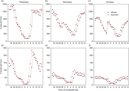
Based on traffic density information (Fig. 4), there are pronounced diurnal and weekly variations in the source strength of vehicle emissions. Since traffic densities observed on ‘working days’ (Monday–Friday) exhibit similar diurnal patterns (not shown), they have been grouped together (Fig. 4a and d). Working days were characterised by a strong day/night contrast in traffic density, rapid changes around sunrise/sunset, and a discernible lunchtime hiatus. Weekend days, on the other hand, were characterised by lower day/night contrasts in traffic density, lower peak volumes, and more gradual changes around sunrise/sunset. The most pronounced seasonal change in traffic density is the 1-hour lag brought about by the change to daylight-savings time from winter to summer. For the purpose of the traffic density plots seasons have been defined as follows: winter (November–March) and summer (May–September).

Fig. 4 Seasonal comparison (winter and summer) of Bern diurnal traffic density (passenger cars and trucks) for weekdays, Saturdays and Sundays.

As one of the main aims of this study is to characterise the influence of atmospheric stability on observed pollution concentrations, it is first necessary to estimate the degree to which weather conditions influence the source strength of emissions (vehicle numbers). To this end, we used the stability classification scheme described in Section 2.2 to subdivide the Bern traffic density information (for cars and trucks combined) by season and day of the week (Fig. 5). As described in Chambers et al. (2015a), the most ‘stable’ nocturnal conditions are typically followed by days with clear-sky, low-wind, anti-cyclonic conditions (i.e. fair weather), whereas near-neutral nights are typically followed by days with significant cloud cover and windy conditions (i.e. inclement weather associated with passing fronts or storms; see also Section 3.4).

Fig. 5 Diurnal cycles of Bern total traffic density as a function of season (winter and summer), day of week and atmospheric stability.

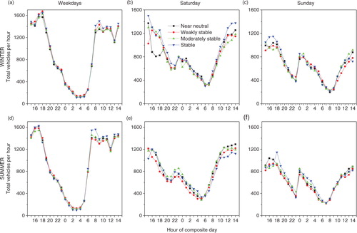
No significant influence of weather conditions upon the working-day traffic density was observed in either summer or winter (Fig. 5a and d). However, on Saturdays there was, on average, a 24 % increase in traffic density between 1000 and 1800 h on fair-weather days (where the preceding night was stable) compared to inclement weather (near-neutral) days in winter; in summer, there was a marked reduction in Saturday traffic density for fair-weather days compared to all other conditions. On Sundays in winter there was, on average, a 24 % higher traffic density around 1800 h on days with the best weather conditions, and a 13 % increase in traffic around 1600–1700 h on inclement days. These variations observed on weekends are likely due to weather-related changes in the patterns of public recreational activities (skiing, cycling etc.).

As the main focus of this paper is on atmospheric mixing influences on pollutant concentrations, unless otherwise stated the remainder of the results will focus just on weekdays (Monday–Friday).

3.2. Overview of climatological influences and fetch histories

Bern daily mean temperatures were below 5° C (and occasionally below 0° C) from November through February (Fig. 6a). This is the most likely period for snow cover, high soil moisture and/or partially frozen soils contributing to a reduced radon source function (see Section 2.2 and Fig. 3b). Mean monthly concentrations of vehicle and domestic heating emissions (e.g. CO and benzene) exhibited peak values in February and November, with minimum concentrations in mid-summer and mid-winter (Fig. 6e and f). This concentration variability was largely influenced by seasonal changes in non-vehicle-related source strengths (e.g. domestic heating usage lower in summer) and synoptic-scale atmospheric ‘flushing’ or stagnation, as evidenced by low monthly-mean wind speeds in February/November and high values in December/January (Fig. 6b).

Fig. 6 (a, b, c, e, f) Monthly distributions (10/50/90th percentiles) of hourly meteorological and pollutant observations; and (d) monthly mean observed, fetch-related and diurnal components of Bern radon data.

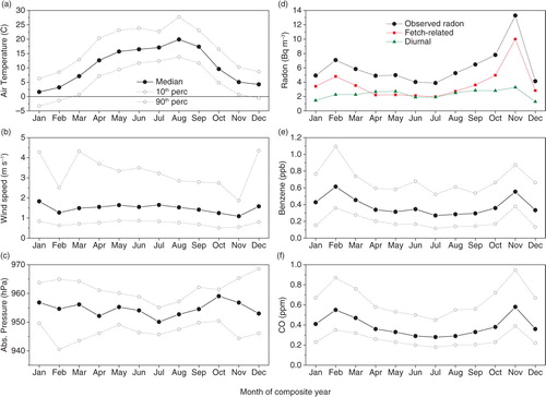
Mean monthly radon concentrations also peaked in February and November, with November being significantly higher (Fig. 6d). Also shown in this panel are the diurnal (green line) and fetch-related (red line) components of the radon signal (see Section 2.2 and Chambers et al., 2015a, 2015b). In both cases, these represent monthly means based on daily averages of the ‘diurnal’ and ‘fetch-related’ components of the radon time series. When the diurnal and fetch-related contributions to the radon time series are separated, it is evident that the largest contributing factor to the observed variations in the monthly mean radon and pollutant concentrations is related to synoptic influences, most likely changes in the air mass fetch history and/or the maximum depth of the daytime atmospheric boundary layer (ABL). This was confirmed by an investigation of 5-day back trajectories and calculated air mass time-over-land covering the measurement period, using the NOAA HYSPLIT v4 model (Draxler and Hess, 1998). The diurnal contribution is significantly smaller, with low values noted in December and January, as well as an increasing trend from July to November (green line).

3.3. Seasonality of diurnal mixing and pollutant patterns

As seen in the seasonally resolved diurnal composite week day radon concentrations (Fig. 7a), the time when the stable nocturnal boundary layer (SNBL) first begins to break down due to the onset of convection changes from 0500 h in summer to around 0800 h in winter. In the afternoon, accumulation of near-surface emissions first begins at around 1600 h in autumn and winter, but not until 1800 h in summer and spring. There was little significant seasonal difference in week day traffic density apart from the daylight-savings time-shift in winter (Fig. 7b).

Fig. 7 Hourly mean diurnal composites by season: (a) diurnal radon, (b) total traffic density (cars + trucks), (c) benzene and (d) CO. Results are for weekdays only.

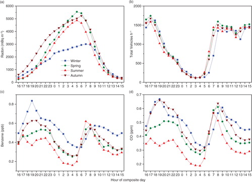
The diurnal cycles of benzene and CO concentrations for each season (Fig. 7c and d) are characterised by a rapid increase in the early morning, beginning with the onset of higher traffic density, reaching a mid-morning peak value when the traffic density reaches its daytime plateau. Beyond this morning peak, concentrations decline into the afternoon due to a deepening mixed layer while the traffic density remains relatively constant. Concentrations then rise once more in the late afternoon in accordance with the peak traffic density, which occurs between 1700 and 1800 h (Fig. 5a and d), together with the decay of convective mixing. After 1800 h, pollution concentrations initially remain elevated despite the reducing traffic density. When vehicle numbers drop to a minimum after 2300 h, however, the composite CO and benzene concentrations both drop very rapidly. Given that the decay half-life of CO is of the order of weeks even in highly polluted air (ATSDR, 2012), these rapid reductions in pollutant concentrations probably indicate the influence of horizontal advection of cleaner air from outside the Bern city area late at night.

In comparison, Quan et al. (2014) reported a diurnal CO cycle for Beijing in winter characterised by minimum values in the early afternoon, but consistently high values throughout the night until sunrise. This may be attributable in part to CO being derived from additional sources other than vehicles (e.g. coal-based domestic heating), but it may also be due to a lack of ‘flushing’ by cleaner air at night in larger cities. As well as the night-time reductions observed in the present study, mean CO concentrations are low compared with the population. Hien et al. (2014) proposed a relationship between population density and vehicle-related benzene pollution based on measurements in Hanoi, Vietnam. Based on this model, Bern – with a population density of 2500 inhabitants km⁻² – should have a mean annual benzene concentration of around 1.25 ppm; which is considerably higher than the observed value of 0.43 ppm. The difference may be partially attributable to the greater number of vehicles (primarily motorbikes) per person in cities like Hanoi, but may also be associated with horizontal advection of clean air from the countryside at night in cities that have compact urban centres like Bern. This aspect will be explored further in Section 4.

Of particular interest in Fig. 7 is that (a) in spring and summer, peak diurnal pollutant concentrations were recorded in the morning, whereas in autumn and winter the peak values were recorded in the afternoons, and (b) the evening peaks are broader (of longer duration) than the morning peaks. These characteristics are due to a combination of changing times of peak traffic density and differences in the atmospheric mixing state. In spring and summer the morning increase in traffic density occurs one hour earlier than in winter (see Fig. 5 and 6) due to daylight saving. At this time of the morning the nocturnal stable layer is still present, although it is beginning to be eroded from below by the young convective boundary layer (CBL). The increased emissions into this still relatively shallow mixing layer temporarily lead to high peak concentrations, which then get quickly dissipated when the CBL begins to grow more rapidly. On average, peak benzene concentrations reach 0.62 ppb on summer mornings, but remain above 0.5 ppb for only 2 hours (Fig. 7c). On spring and summer evenings, peak traffic emissions occur before the SNBL has become well established, such that the mixing volume is still comparatively large, resulting in a modest evening pollutant peak. In autumn and winter, on the other hand, the SNBL is better established at the time of evening peak emissions, resulting in a reduced mixing depth and higher peak concentrations. In the absence of convection driven by surface heating, vertical mixing is severely reduced at night and the evening autumn/winter peak pollutant levels are diluted only by horizontal advection and lateral diffusion, resulting in an extended period of high concentrations. On average, peak benzene concentrations reach 0.85 ppb on winter evenings, and remain above 0.5 ppb for 9 hours (Fig. 7c).

Despite a slightly lower daytime traffic density in winter compared to the other seasons (Fig. 7b), daytime pollutant concentrations in winter were almost double the corresponding summer values (Fig. 7c). Furthermore, despite low traffic densities in the early morning (0300–0400 h), nocturnal benzene and CO concentrations were considerably higher in winter than summer. This is most likely attributable to seasonal changes in the depth of both the nocturnal and the daytime ABL, with the larger pollutant concentrations indicating shallower mixing depths in winter, consistent with Collaud Coen et al. (2014). The fact that the diurnal radon composite (Fig. 7a) shows values that are significantly lower in winter than in the other seasons points to a substantially reduced radon flux in winter, as discussed in Section 2.2 (and consistent with the map of Karstens et al., 2015).

3.4. Meteorological characterisation of radon-derived stability categories

The nocturnal atmospheric mixing state (stability) at any given time derives from a combination of mechanical mixing (interaction between wind speed and surface roughness elements) and thermal stratification. Unfortunately, only near-surface temperature (not temperature gradient) data was available in Bern, examples of which, separated by radon-derived stability category, are provided in Fig. 8.

Fig. 8 Diurnal temperature (relative to the morning minimum value) at Bern in winter and spring as a function of radon-derived stability category.

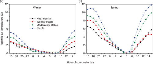
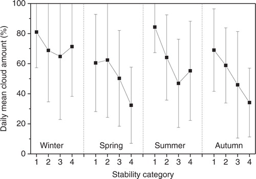
As the most stable nocturnal conditions tend to be associated with clear-sky conditions, and near-neutral conditions with significant cloud cover, an increase in amplitude of the diurnal temperature cycle, and rate of atmospheric heating in the morning, was noted with increasing atmospheric stability classification. To further demonstrate this point, Fig. 9 shows a clear reduction in daily mean cloud amount (as observed 4.5 km northeast of the Bern pollution monitoring site) with increasing nocturnal atmospheric stability. On average, between 1000 and 1500 h following a night classified as well-mixed (near-neutral conditions), there was between 28 and 37% more cloud cover than for corresponding periods classified as stable. Furthermore, the duration of cloud cover (as a percent of each hour) was between 45 and 59% higher for day times following well-mixed nocturnal conditions. This is consistent with more stratiform cloud cover following well-mixed nights and fair-weather cumulus following stable nights.

Fig. 9 Seasonal breakdown of the change in daily mean cloud cover with stability classification (1: well mixed/near neutral; 2: weakly stable; 3: moderately stable; 4: very stable).

In a similar fashion we categorised the 36 m diurnal wind speed observations by season and radon-derived stability category (Fig. 10). Overall, well-mixed conditions were typically associated with nocturnal wind speeds of 1.4–3.3 m s⁻¹, whereas the nocturnal wind speeds of stable nights typically varied from 0.7 to 0.9 m s⁻¹. These results are consistent with those of Quan et al. (2014), Grundstrom et al. (2015), Pitari et al. (2015), Sesana et al. (2006) and Chambers et al. (2011, 2015a), who each associated stable nocturnal conditions (including morning haze events) with wind speeds less than 1–1.5 m s⁻¹.

Fig. 10 Hourly mean diurnal composites of wind speed by season and stability classification.

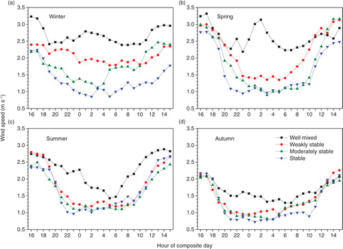
In winter (Fig. 10a), and to a lesser extent spring (Fig. 10b), a clear distinction was observed between nocturnal wind speeds of each stability category: well-mixed conditions were characterised by the highest nocturnal mean wind speeds (around 2.5 m s⁻¹), whereas stable conditions were typically characterised by nocturnal mean wind speeds of ≤1 m s⁻¹. Quan et al. (2014) noted that haze events in Beijing were often associated with wind speeds less than 1 m s⁻¹. In summer and autumn, on the other hand, while the well-mixed nights were characterised by the highest wind speeds (>1.5 m s⁻¹), there was little distinction between wind speeds from moderately mixed to stable atmospheric conditions. Grundstrom et al. (2015) found that up to 93% of pollutant concentration variability can be attributed to conditions for which wind speed <1.5 m s⁻¹.

These results indicate that changes in mechanical mixing represent the dominant influence on the nocturnal mixing state in winter and spring (Fig. 10), whereas changes in the thermal stratification of the lower atmosphere are the dominant influence on the nocturnal mixing state in summer and autumn (Fig. 8 and 9). Fig. 9 shows a considerably larger reduction in daily mean cloud amount with stability in summer and autumn than for winter, which would facilitate nocturnal surface radiative cooling and the development of strong thermal stratification of the lower atmosphere.

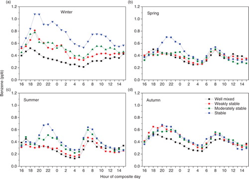
Fig. 11 Hourly mean diurnal composites of benzene concentration by season and stability category (weekdays only).

3.5. Stability classification of emissions

As for the climatological data, we separated the benzene (Fig. 11) and CO (Fig. 12) concentrations by season and radon-derived stability category. While there was typically little significant difference in afternoon (1400–1600 h) pollutant concentrations within each season, nocturnal concentrations – particularly either side of the early-morning traffic density hiatus (Fig. 5) – spread out very clearly according to stability, with the highest values found under stable atmospheric conditions, and the lowest in ‘well-mixed’ conditions. In the winter composite diurnal cycle, peak benzene concentrations under stable conditions ( 1.1 ppb) were 120% higher than for near-neutral (well-mixed) conditions (0.5 ppb). By comparison, summertime peak benzene concentrations increased by 53% from well-mixed (0.45 ppb) to stable nocturnal conditions (0.7 ppb).

Fig. 12 Hourly mean diurnal composites of carbon monoxide concentration by season and stability category (weekdays only).

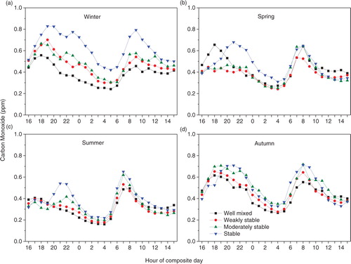
On average, for the defined stability categories, mid-evening (2000–2200 h) concentrations of benzene and CO were frequently a factor of 2–2.5 higher under stable as opposed to well-mixed conditions. As evident in Fig. 10, a change of wind speed of corresponding magnitude was observed between the stability categories. The weakest distinction between categories occurred in autumn, when there was also the smallest range of wind speeds at night (Fig. 10). Quan et al. (2014) also reported enhanced CO concentrations in Beijing under conditions of reduced atmospheric mixing. Occasional instances when the well-mixed concentrations exceed those of stable conditions (e.g. in Fig. 11b and 12b) may be attributable to transport of polluted air from beyond the ‘local’ region of influence.

Apart from the stability-related variations in signal amplitude discussed above, in general similar features in the diurnal patterns of variability in pollutant concentrations were apparent in the stability-separated results than were seen in the combined results discussed in Section 3.3 (Fig. 7). This includes the rapid reductions in pollutant concentrations late at night. Specific features of these diurnal patterns of pollutant concentrations will be analysed further in the next section.

4. Separating emission patterns and atmospheric effects

Given the results presented in Section 3, we can hypothesise that nocturnal air quality in the Bern city centre is principally controlled by interplay between three time-varying processes: local traffic emissions within the city area, vertical dilution by boundary layer mixing (controlled by atmospheric stability) and horizontal advection of cleaner air from outside the central urban/industrial area. In this section, we attempt to separate these aspects in order to isolate the part that is due to local emissions, by applying a simple box model to the seasonally resolved diurnal composites. This enables a direct comparison between hourly traffic density observations and vehicle emissions.

4.1. Radon-based box model with advection

Consider an idealised box model for the case of some trace gas ‘x’ mixing within a well-defined SNBL of ‘effective’ depth h (i.e. assuming a well-mixed profile), with a locally well-distributed surface source function F _x and an internal sink characterised by an exponential function with temporal decay constant λ _x [s⁻¹]. The box is assumed to be mixed ‘well enough’ that the (measured) surface concentration of ‘x’ can be considered to be representative of the layer-averaged value, , and h is allowed to vary with time and encroach upon a ‘residual’ layer above the SNBL. Horizontal advection is modelled using a simple exponential drop-off of P _x upstream, assuming no changes in the depth or characteristics of the mixing layer: where d [m] is distance upstream and γ _x [m⁻¹] is the spatial decay constant. With these assumptions, the budget for the layer-integrated trace gas, P _x h, can be written as:1

where is a temporal decay constant representative of the combined effects of internal sinks and horizontal advection, with U the layer-averaged wind speed. If the concentration of ‘x’ in the encroached residual layer (just above z=h) at time t, which is modelled as: where is the measured value of p _x in the previous late afternoon (before the SNBL starts to form). On the other hand, if the concentration of ‘x’ in the air left behind by the shrinking SNBL, which is modelled as: . If surface emissions F _x can be assumed to be approximately constant over some short time interval [t ₀, t], then eq. (1) can be solved analytically to yield an expression for P _x h at time t given knowledge of the previous state (at t ₀ ):2

where . Note that . The three terms on the right hand side of eq. (2) respectively describe the amount of ‘x’ added by surface emissions, remaining as a decayed legacy, and exchanged by encroachment or shrinking in the SNBL column during the current time step. If h=h ₀, eq. (2) reduces to: . Therefore, the sign of was used to decide whether the layer is growing or shrinking during the time interval, and thus which form of to use.

Equation (2) can be rearranged to yield expressions for either h or F _x . Our approach will be to apply it twice: firstly for the case of radon, in order to obtain an estimate for h; and secondly for the case of a pollutant of interest (benzene or CO), in order to estimate F _x using h obtained from the first step. We note that the actual physical interpretation of the radon-based length scale h (i.e., the ‘effective’ SNBL depth assuming a well-mixed profile) is largely irrelevant in this approach, as h is merely a convenient intermediary that ‘drops out’ of the process when estimating F _x in the second step. This approach, designed for the case of diurnal pollution fluxes in a small city, can be considered to be a generalisation of both the well-known ‘radon calibration’ technique, used to obtain regional flux estimates [e.g. Zahorowski et al., 2004; eq. (7)], and the ‘nocturnal storage-ratio’ method, used to estimate nocturnal fluxes at the field scale using a similarly distributed reference species (e.g. Pendall et al., 2010; Kelliher et al., 2002; Laubach et al., 2015).

4.2. Radon-based nocturnal mixing length scale

For the case of radon, following the discussion in the Introduction we can reasonably approximate F _x as constant on the spatial scale of Bern and its immediate surroundings, and also in seasonally averaged composite diurnal statistics (i.e., F _x known and γ _x =0). Seasonal mean radon fluxes were calculated using the 0.083° resolution European radon flux map of Karstens et al. (2015) for 2011: 16.1, 23.6, 33.5 and 32.6 mBq m⁻² s⁻¹ for winter, spring, summer and autumn, respectively. Rearranging eq. (2), we obtain a method for calculating h that is similar to that of Fontan et al. (1979), Sesana et al. (2003) and Griffiths et al. (2014). Starting with a nominal small value of 10 m at 1600 h, we then computed the evolution of h over the course of the night (Fig. 13c and d).

Fig. 13 Seasonally separated nocturnal composites of (a, b) radon concentrations, (c, d) box-model-derived SNBL depths (note logarithmic scale), (e, f) wind speed and (g, h) wind direction, for very stable (left) and weakly stable (right) conditions in Bern.

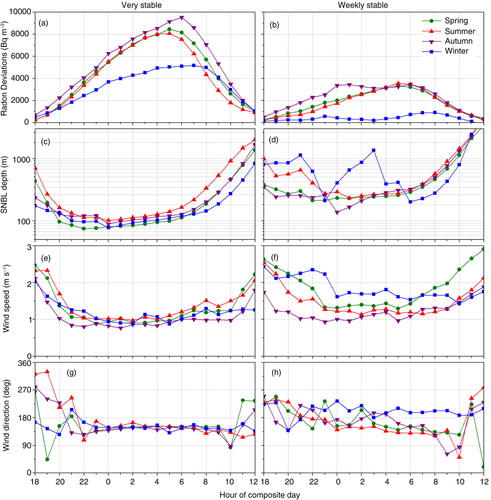
For the ‘very stable’ stability category (Fig. 13a, c, e and g), the method produces well-defined SNBL depth curves evolving similarly through the course of the night, with a minimum value below 100 m being reached around midnight, and then slow growth over the remainder of the night. When the radon concentrations start to drop after sun rise, signalling the start of convective mixing and the erosion of the SNBL, h grows more rapidly as radon is diluted into the developing daytime boundary layer. Despite the markedly smaller radon concentrations observed in winter (Fig. 13a), calculated SNBL depths for winter fall within the range of the other seasons (Fig. 13c), confirming the efficacy of employing the seasonal flux variation of Karstens et al. (2015). Both wind speed and direction are remarkably stable throughout the night in this category for all seasons (Fig. 13e and g). In the ‘weakly stable’ category (Fig. 13b, d, f and h), the SNBL depth curves are only well-defined in spring and summer, with minimum values in the range 150–250 m. Both wind speed and direction are more variable in this category, diurnally and seasonally (Fig. 13f and h). In autumn, elevated radon values in the first half of the night (up until about 0200 h), interpreted by the model as lower h values, are likely associated with lower wind speeds during the same period (Fig. 13f), whilst relatively elevated wind speeds throughout the night in winter prevent a strong nocturnal build-up of radon resulting in a failure of the model to reliably compute h (Fig. 13b and d). In the ‘moderately stable’ category (not shown), results are intermediate between the ‘very stable’ and ‘weakly stable’ categories. The ‘well-mixed’ category was not diagnosable using this model, due to the absence of a nocturnal build-up of radon.

4.3. Simulated vehicle emission patterns

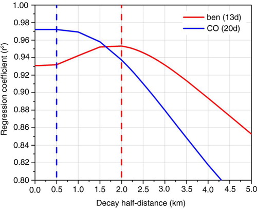
With h known, and again starting at 1600 h, eq. (2) was rearranged to obtain expressions (not shown) for the time-varying surface source functions F _x for benzene and CO in Bern. The resulting simulated time histories for F _x during the central night-time period 2000–0600 h were regressed against the total vehicle count (TVC), in order to quantify the degree to which the idealised box model explained the nocturnal variance in the measured pollutant concentrations. This assumes that TVC is an accurate proxy for integrated vehicle emissions. As a first step in this process, the model was optimised to find the values of parameters λ _x and γ _x that yielded the best least-squares regression coefficients (r²) between F _x and TVC for the well-simulated case of benzene and CO concentrations in spring ‘very stable’ conditions. A range of previously reported λ _x values for benzene (ATSDR, 2007) and CO (ATSDR, 2012) were tested, and it was found that in both cases the model results were largely insensitive to the value used. Final half-lives chosen (and used in all calculations) were 13 d for benzene and 20 d for CO. On the other hand, it was found that the results were highly sensitive to the value chosen for γ _x . Figure 14 shows least-squares regression coefficients resulting from simulations with a range of values for γ _x , expressed as half-distances. An optimum decay half-distance of around 2 km is found for benzene, which fits very well with the average radius of Bern being around 4 km (see Fig. 1; also considering a total area of 51.6 km² as noted by van der Laan et al., 2014). On the other hand, correlation coefficients for CO increase for decreasing half-distances, until a broad plateau is reached for all values below about 1 km. The final half-distance chosen for CO was 0.5 km. This shorter relaxation distance for CO compared with benzene seems to indicate a very local source for CO. This is likely to be incomplete combustion associated with idling vehicles, and possibly residential heating, in the central city district close to the measurement site. As noted in the study of van der Laan et al. (2014), a significant fraction of the fossil fuel-based emissions in Bern are known to be from natural gas combustion associated with residential heating (e.g. 28% for CO₂). The larger relaxation distance for benzene, on the other hand, may be attributable to advection of vehicle emissions from a much broader region, encompassing the whole Bern city area and possibly including regional motorways (see Fig. 1). Intercity Route 6 (www.google.com.au/maps/@46.9425535,7.4497062,13z), for example, approaches Bern from the south east, which is the predominant up-wind direction at night (Fig. 13g and h).

Fig. 14 Least-squares regression coefficients of the correlation between pollutant fluxes (CO; benzene) computed by the box model and measured total vehicle counts in Bern city centre, for a range of values of the spatial decay parameter γ _x (expressed as a half-distance). Only very stable nights in spring were used in these tests, and pollutant half-lives were held constant at 20 d for CO and 13 d for benzene. Optimised γ _x values used in the box model are indicated with vertical dashed lines.

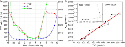
Again using the case of benzene in spring ‘very stable’ conditions, Fig. 15 illustrates the excellent results that are obtainable with this technique. When SNBL depths are stable or only slowly changing during the central part of the night (2000–0600 h), the computed benzene flux tracks the TVC very closely (Fig. 15a). This leads to a linear correlation with a high regression coefficient (r²~0.95), indicating that the model explains most of the variance in the benzene signal (Fig. 15b). As the SNBL erodes after sun rise and the trapped radon and pollutants are dispersed into the fast-growing daytime CBL, however, the assumptions of the budget model no longer hold and it fails to predict the benzene flux adequately after about 0800 h (Fig. 15a and b inset).

Fig. 15 Box model results for benzene in Spring ‘very stable’ conditions in Bern. (a) Time series of computed benzene flux on right axis and measured total vehicle counts (TVC) on left axis; also shown is computed SNBL depth, h, on left axis; (b) computed benzene flux versus measured TVC during the period 2000–0600 h, marked with vertical dashed lines in (a). Linear fit is indicated in red; inset shows the entire period 1800–1200 h.

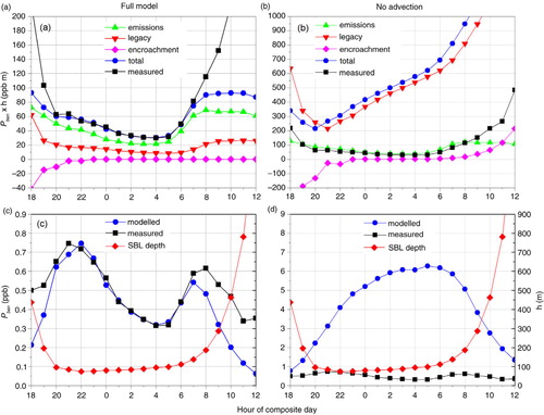
Outside of the central night period (2000–0600 h), the TVC data could presumably still be used to obtain a reasonable estimate for the surface benzene emissions, using the slope and intercept values obtained from the night-time regression. Calculating the 24-hour benzene emissions in this way and then applying them to the model equations along with the radon-derived SNBL depth, enabled a semi-independent prediction of the entire diurnal benzene evolution. This allowed an opportunity to explore the model's behaviour a little more deeply. In Fig. 16, the three components [RHS of eq. (2)] of the layer-integrated benzene (P _ben h) are calculated and plotted together with the predicted and measured benzene values, for both the full model (Fig. 16a and c) and a version of the model without the advection term (γ _x =0; Fig. 16b and d). In the full model, strong advection of cleaner air prevents the legacy term (amount of pollutant remaining in the layer from the previous time step) from growing, despite the continuous input of new surface emissions. In addition, the encroachment term stays small even in the morning growth period, because pollutant concentrations in the residual layer have dropped to negligible values (again due to advection). This leads to the observed behaviour of dropping near-surface benzene levels in the central part of the night, despite the steady SNBL depth and the long residence time of benzene in the atmosphere (Fig. 16c). In strong contrast, when the model is employed without advection (Fig. 16b and d), the legacy term steadily climbs throughout the night and the encroachment term becomes significant after sunrise. This leads to predicted near-surface benzene levels that are 12 times higher than measured levels by the end of the night, and only start to drop when the mixing depth rises sharply after dawn (Fig. 16d).

Fig. 16 Comparison of box model behaviour with (a, c) and without (b, d) horizontal advection, for Spring ‘very stable’ conditions. (a, b) Component terms for layer-integrated benzene (P _ben h) over the extended period 1800–1200 h, using pre-estimated fluxes (F _ben ) and radon-based SNBL depths (h). F _ben was calculated from TVC using regression results from the full model during the well-simulated period 2000–0600 h. (c, d) Modelled and measured P _ben and h values.

4.4. Seasonal and stability-related variations in emissions

Results from the regressions of simulated F _x values against measured TVC during the central night-time period 2000–0600 h are tabulated in Table 1. With the horizontal advection term in use, very high regression coefficients are found in spring and summer for both benzene (r² ~ 0.90–0.96) and CO (r² ~ 0.88–0.98) in the two highest stability categories. In autumn and winter, the ‘very stable’ r² values remain fairly high whilst the ‘moderately stable’ values drop substantially. In the ‘weakly stable’ category, very high regression coefficients are only seen in spring, dropping to values around 0.8 in summer and autumn, and then low values in winter.

Table 1. Regression results for box-model-simulated pollutant fluxes (F _x ) versus measured total vehicle count (TVC) in Bern, by stability category and season

		Regression coefficient (r^2)				Gradient [F x ] per [veh h^−1]				Offset [F x ]
Regression (F x vs. TVC)	Stability category	Spring	Summer	Autumn	Winter	Spring	Summer	Autumn	Winter	Spring	Summer	Autumn	Winter
	Weakly stable	0.9300	0.8099	0.8124	0.3998	0.4954	1.2057	0.5546	3.7596	284.1	−10.6	205.2	773.4
Benzene flux	Moderately stable	0.9002	0.9382	0.8446	0.5163	0.3472	0.6825	0.2090	0.2639	78.1	66.4	233.6	587.1
F b [µg m^−2 h^−1]	Very stable	0.9532	0.9603	0.9699	0.8439	0.1987	0.5063	0.2948	0.3405	93.6	55.6	71.7	202.4
	Weakly stable	0.9019	0.8185	0.8185	0.3051	0.5750	1.4922	0.7314	3.6271	491.8	107.4	337.1	1464.7
CO flux	Moderately stable	0.8759	0.9686	0.8494	0.6007	0.4970	0.6246	0.2871	0.3244	131.6	158.7	377.6	746
F c [mg m^−2 h^−1]	Very stable	0.9720	0.9756	0.9388	0.9243	0.2241	0.4650	0.3796	0.3752	145.5	113.5	138.1	230.5

The high correlations in spring and summer indicate both that the extended box model produces a good representation of the effective benzene and CO emissions in Bern city centre during those seasons, and that the emissions are explained mainly by vehicular traffic at this site. The fact that correlations are always highest in the ‘very stable’ cases, and remain high throughout all seasons of the year, is likely due to the near-calm wind conditions (Fig. 10) and strong thermal suppression; this leads to very low turbulence levels, limiting mixing to only the close locality of the measurement site (a busy intersection). On the other hand, the reduced correlations in winter likely indicate an enhanced influence from pollution sources that are unrelated to vehicular emissions. The flux offset values produced by the linear regressions also increase substantially in winter for the ‘moderately stable’ and ‘weakly stable’ cases (Table 1), providing further support for this hypothesis. It should be noted, however, that no attempt was made to remove ‘background’ concentrations of benzene or CO from the Bern pollution time series, which also likely contributes to the non-negligible offset values in the regression results depicted in Table 1.

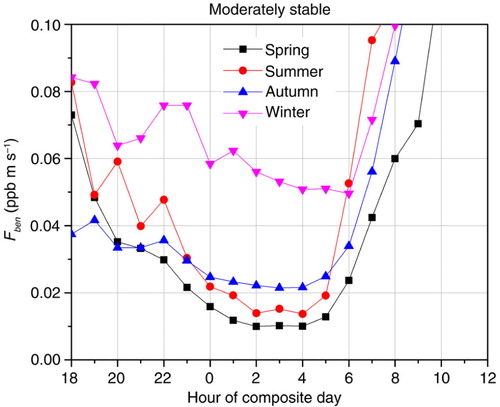
Figure 17 shows simulated benzene flux diurnal composites for all four seasons for the ‘moderately stable’ case. Comparison with Fig. 7b confirms a strong similarity to the TVC evolution during spring and summer, whilst the winter evolution is dissimilar in shape and substantially elevated (relative to spring and summer) over the whole night. Hour-to-hour variability in the first half of night (1800–0000 h) may indicate heterogeneous local sources, after which emissions become steadier for the rest of the night. In contrast, although the autumn fluxes are somewhat elevated in the second half of the night (0000–0600 h), they are actually lower than the spring and summer fluxes in the first half of the night. This corresponds to a period of different (lower) wind speeds seen in the autumn meteorological data for the moderately stable case (not shown, but similar to Fig. 13f), so it could perhaps be associated with a slightly different fetch region for this case.

Fig. 17 Simulated benzene fluxes for Bern in moderately stable conditions by season.

Major anthropogenic sources of benzene in Switzerland have been estimated (BUWAL, 2003; INFRAS/Meteotest, 2013) to be 62–69% road traffic (including fuel handling facilities), 32–15% heating (mainly wood fires, but also oil and gas) and 7–17% Industry (including off-road engines). Of these sources, domestic heating would be expected to be significantly enhanced in wintertime. For CO, the likely additional source in Bern is incomplete natural gas combustion, again associated with enhanced wintertime domestic heating (ATSDR, 2012; van der Laan et al., 2014).

When regression coefficients are high (>0.9), the gradient values presented in Table 1 provide a strong relationship between traffic volume (TVC) as measured at the NABEL road-curb monitoring site, and total benzene and CO emissions associated with vehicles in the area of the Bern city centre. Considering only the most stable category, average gradient values for benzene (CO) were found to be 0.335±0.129 µg m⁻² h⁻¹ (0.361±0.100 mg m⁻² h⁻¹) per vehicle h⁻¹. During daytime (TVC~1500 veh h⁻¹ past the NABEL site; Fig. 7b), this corresponds to integrated vehicle emissions of around 0.503 (542) kg km⁻² h⁻¹ for benzene (CO) in the Bern city centre area. For both pollutants, emissions relative to the measured TVC tend to be a little higher in summer than in the other seasons, and there is also a small trend towards higher emissions per TVC for lower stability classes in both spring and summer. These effects could be indicative of shifts in the effective fetch region of the pollution measurements for different seasons and stabilities, which would lead to corresponding changes in the relationship between TVC as measured at the NABEL site and traffic density in the wider city region. Further investigation of these effects would be interesting, but is beyond the scope of the present study.

5. Conclusions

We analysed 13 months of hourly traffic density, radon, benzene and CO concentrations together with climatological data, in order to quantify the influence of changing atmospheric conditions and traffic density on air quality in Bern, Switzerland. As part of our investigations, we adapted a recently developed radon-based technique for assessing nocturnal atmospheric stability (Chambers et al., 2015a, 2015b), in order to account for seasonal changes in day length and reductions in the local radon source function as a result of snow/ice cover and soil moisture effects in winter. Weekdays became the focus of this study, as their traffic density was found to be most consistent across all seasons and atmospheric stability regimes.

Seasonal cycles of pollutant concentrations were found to be strongly influenced by site climatology (changing fetch, wind speed and mixing depth), whereas diurnal pollutant cycles reflected an interplay between variations in source strength (e.g. traffic density), the depth of the atmospheric mixing layer and local horizontal advection of cleaner air from outside the central urban/industrial area of this small compact inland city. Due to a combination of seasonal changes in day length and daylight-savings time in relation to traffic patterns, substantial seasonal differences were noted in both the time and duration of peak pollutant concentrations within the diurnal cycle. For example, on average in summer the peak diurnal benzene concentrations (0.62 ppb) occurred in the morning and remained above 0.5 ppb for 2 hours, whereas in winter the average peak concentrations (0.85 ppb) occurred in the evening and remained above 0.5 ppb for 9 hours.

Throughout winter and spring, wind speed was found to have the largest influence on nocturnal atmospheric stability (stable: 0.7–0.9 m s⁻¹; near-neutral: 1.4–3.3 m s⁻¹), whereas thermal stratification of the lower atmosphere was the dominant influence in summer and autumn, as evidenced by an analysis of cloud cover and solar irradiance data. In the winter composite diurnal cycle, peak benzene concentrations under stable conditions (1.1 ppb) were 120% higher than for near-neutral (well-mixed) conditions (0.5 ppb). By comparison, summertime peak benzene concentrations increased by 53% from well-mixed (0.45 ppb) to stable nocturnal conditions (0.7 ppb).

An idealised box model incorporating a simple advection term was used to derive a nocturnal mixing length scale based on radon, and then inverted to simulate composite diurnal variations in benzene and CO emissions in the city centre. This method effectively removes the influences of local horizontal advection and stability-related vertical dilution, enabling a direct comparison with hourly traffic density. It should be noted that the method is only expected to work well on average (in this case, seasonally), and is therefore not intended as an alternative to high-resolution modelling but rather as a complementary integrative (‘top-down’) approach. With the advection term calibrated appropriately and radon fluxes taken from Karstens et al. (2015), excellent results were obtained, with high regression coefficients in spring and summer for both benzene (r² ~0.90–0.96) and CO (r² ~0.88–0.98) in the two highest stability categories. Weaker regressions in winter likely indicate additional contributions from combustion sources unrelated to vehicular emissions. Average vehicular emissions during daylight hours were estimated to be around 0.503 (542) kg km⁻² h⁻¹ for benzene (CO) in the Bern city centre.

6. Acknowledgements

We thank Ot Sisoutham and Sylvester Werczynski at the Australian Nuclear Science and Technology Organisation for their support in constructing the detector and developing the monitoring software for the radon measurement program at Bern. We also thank Markus Leuenberger and Peter Nyfeler at the Physics Institute of the University of Bern, for hosting and supporting the operation of the radon detector.

References

- Allegrini I., Febo A., Pasini A., Schiarini S. Monitoring of the nocturnal mixed layer by means of particulate radon progeny measurement. J. Geophys. Res. 1994; 99: 18765–18777. DOI: http://dx.doi.org/10.1029/94JD00783.
- ATSDR. U.S. Department of Health and Human Services, Public Health Service, Agency for Toxic Substances and Disease Registry (ATSDR). Toxicological Profile for Benzene. 2007. Online at: http://www.atsdr.cdc.gov/ToxProfiles/TP.asp?id=40&tid=14.
- ATSDR. U.S. Department of Health and Human Services, Public Health Service, Agency for Toxic Substances and Disease Registry (ATSDR). Toxicological Profile for Carbon Monoxide. 2012. Online at: http://www.atsdr.cdc.gov/ToxProfiles/TP.asp?id=1145&tid=253.
- Avino P. , Brocco D. , Lepore L. , Pareti S . Interpretation of atmospheric pollution phenomena in relationship with the vertical atmospheric remixing by means of natural radioactivity measurements (radon) of particulate matter. Ann. Chim. 2003; 93(5–6): 589–594.
- Beatty T. K. M. , Shimshack J. P . Air pollution and children's respiratory health: a cohort analysis. J. Environ. Econ. Manage. 2014; 67(1): 39–57.
- Belušić A., Herceg-Bulić I., Bencetić Klaić Z. Using a generalized additive model to quantify the influence of local meteorology on air quality in Zagreb. Geofizika. 2015; 32: 47–77. DOI: http://dx.doi.org/10.15233/gfz.2015.32.5.
- Borgie M. , Garat A. , Cazier F. , Delbende A. , Allorge D. , co-authors . Traffic-related air pollution. A pilot exposure assessment in Beirut. Lebanon Chemosphere. 2014; 96: 122–128.
- Bosard M. , Feranec J. , Otahel J . CORINE land cover technical guide – addendum 2000. European Environmental Agency Technical Report. 2000. No. 40, Copenhagen, Denmark.
- BUWAL. Benzol in der Schweiz (Benzene in Switzerland). Schriftenreihe Umwelt Nr. 350. Bundesamt für Umwelt, Wald und Landschaft, Bern. 2003; 38(Suppl.): Online at: http://www.bafu.admin.ch/publikationen/publikation/00514/index.html?lang=de.
- Byrd G. D. , Fowler K. W. , Hicks R. D. , Lovette M. E. , Borgerding M. F . Isotope dilution gas chromatography – mass spectrometry in the determination of benzene, toluene, styrene and acrylonitrile in mainstream cigarette smoke. J. Chromatogr. 1990; 503: 359–368.
- Chambers S. D. , Galeriu D. , Williams A. G. , Melintescu A. , Griffiths A. D. , co-authors . Atmospheric stability effects on potential radiological releases at a nuclear research facility in Romania: characterising the atmospheric mixing state. J. Environ. Radioact. 2016; 154: 68–82.
- Chambers S. D., Hong S. -B., Williams A. G., Crawford J., Griffiths A. D., co-authors. Characterising terrestrial influences on Antarctic air masses using radon-222 measurements at King George Island. Atmos. Chem. Phys. 2014; 14: 9903–9916. Online at: www.atmos-chem-phys.net/14/9903/2014/; DOI: http://dx.doi.org/10.5194/acp-14-9903-2014.
- Chambers S. D. , Wang F. , Williams A. G. , Xiaodong D. , Zhang H. , co-authors . Quantifying the influences of atmospheric stability on air pollution in Lanzhou, China, using a radon-based stability monitor. Atmos. Environ. 2015b; 106: 1–11.
- Chambers S. D., Williams A. G., Crawford J., Griffiths A. D. On the use of radon for quantifying the effects of atmospheric stability on urban emissions. Atmos. Chem. Phys. 2015a; 15: 1175–1190. DOI: http://dx.doi.org/10.5194/acp-15-1175-2015.
- Chambers S., Williams A. G., Zahorowski W., Griffiths A., Crawford J. Separating remote fetch and local mixing influences on vertical radon measurements in the lower atmosphere. Tellus B. 2011; 63: 843–859. DOI: http://dx.doi.org/10.1111/j.1600-0889.2011.00565.x.
- Chattopadhyay B. P. , Mukherjee A. , Mukherjee K. , Roychowdhury A. , Som D . Exposure to vehicular pollution and assessment of respiratory function in urban inhabitants. Lung. 2007; 185(5): 263–270.
- Collaud Coen M., Praz C., Haefele A., Ruffieux D., Kaufmann P., co-authors. Determination and climatology of the planetary boundary layer height above the Swiss plateau by in situ and remote sensing measurements as well as by the COSMO-2 model. Atmos. Chem. Phys. 2014; 14(23): 13205–13221. DOI: http://dx.doi.org/10.5194/acp-14-13205-2014.
- Draxler R. R. , Hess G. D . An overview of the HYSPLIT-4 modelling system for trajectories, dispersion and deposition. Aust. Meteorol. Mag. 1998; 47: 295–308.
- Duenas C. , Perez M. , Fernandez M. C. , Carretero J . Radon concentrations in surface air and vertical atmospheric stability of the lower atmosphere. J. Environ. Radioact. 1996; 31(10): 87–102.
- EC. Directive 2000/69/EC of the European Parliament and of the Council of 16 November 2000 relating to limit values for benzene and carbon monoxide in ambient air. Official Journal of the European Communities. 2000; L313: 12. Online at: http://eur-lex.europa.eu/legal-content/EN/TXT/?uri=CELEX:32000L0069.
- Fan R. , Li J. , Chen L. , Xu Z. , He D. , co-authors . Biomass fuels and coke plants are important sources of human exposure to polycyclic aromatic hydrocarbons, benzene and toluene. Environ. Res. 2014; 135: 1–8.
- Foken T . 50 years of the Monin–Obukhov similarity theory. Boundary-Layer Meteorol. 2006; 119: 431–437.
- Fontan J., Guedalia D., Druilhet A., Lopez A. Une methode de mesure de la stabilité verticale de l'atmosphere pré du sol. Boundary Layer Meteorol. 1979; 17: 3–14. DOI: http://dx.doi.org/10.1007/BF00121933.
- Galmarini S . One year of 222Rn concentration in the atmospheric surface layer. Atmos. Chem. Phys. 2006; 6: 2865–2887.
- Ghose M. K. , Paul R. , Banerjee S. K . Assessment of the impacts of vehicular pollution on urban air quality. J. Environ. Sci. Eng. 2004; 46: 33–40.
- Griffiths A. D. , Conen F. , Weingartner E. , Zimmermann L. , Chambers S. D. , co-authors . Surface-to-mountaintop transport characterised by radon observations at the Jungfraujoch. Atmos. Chem. Phys. 2014; 14: 12763–12779.
- Grundstrom M., Tang L., Hallquist M., Nguyen H., Chen D., co-authors. Influence of atmospheric circulation patterns on urban air quality during the winter. Atmos. Pollut. Res. 2015; 6: 278–285. DOI: http://dx.doi.org/10.5094/APR.2015.032.
- Gulia S., Nagendra S. M. S., Khare M., Khanna I. Urban air quality management – a review. Atmos. Pollut. Res. 2015; 6: 286–304. DOI: http://dx.doi.org/10.5094/APR.2015.033.
- Hien P. D. , Hangartner M. , Fabian S. , Tan P. M . Concentrations of NO2, SO2, and benzene across Hanoi measured by passive diffusion samplers. Atmos. Environ. 2014; 88: 66–73.
- Holford D. J. , Schery S. D. , Wilson J. L. , Phillips F. M . Modeling radon transport in dry, cracked soil. J. Geophys. Res. 1993; 98(B1): 567–580.
- Holtslag A. A. M . Introduction to the third GEWEX atmospheric boundary layer study (GABLS3). Boundary-Layer Meteorol. 2014; 152: 127–132.
- INFRAS/Meteotest. Benzol-Immissionen Schweiz, Modellierung 1990–2020. Im Auftrag des Bundesamtes für Umwelt BAFU. 2013; Bern: Zürich. Online at: http://www.bafu.admin.ch/luft/luftbelastung/11921.
- Karstens U., Schwingshackl C., Schmithüsen D., Levin I. A process-based 222radon flux map for Europe and its comparison to long-term observations. Atmos. Chem. Phys. 2015; 15: 12845–12865. DOI: http://dx.doi.org/10.5194/acp-15-12845-2015.
- Kelliher F. M. , Reisinger A. R. , Martin R. J. , Harvey M. J. , Price S. J. , co-authors A . Measuring nitrous oxide emission rate from grazed pasture using Fourier-transform infrared spectroscopy in the nocturnal boundary layer. Agric. Forest Meteorol. 2002; 111: 29–38.
- Kim K. , Pandey S. K. , Kabir E. , Susaya J. , Brown R. J. C . The modern paradox of unregulated cooking activities and indoor air quality. J. Hazard. Mater. 2015a; 195: 1–10.
- Kim K., Sul K., Szulejko J. E., Chambers S. D., Feng X., co-authors A.Progress in the reduction of carbon monoxide levels in major urban areas in Korea. Environ. Pollut. 2015b; 207: 420–428. DOI: http://dx.doi.org/10.1016/j.envpol.2015.09.008.
- Koffi E. N., Bergamaschi P., Karstens U., Krol M., Segers A., co-authors.Evaluation of the boundary layer dynamics of the TM5 model. Geosci. Model Dev. Discuss. 2016. DOI: http://dx.doi.org/10.5194/gmd-2016-48.
- Kondo H. , Murayama S. , Sawa Y. , Ishijima K. , Matsueda H. , co-authors . Vertical diffusion coefficient under stable conditions estimated from variations in the near-surface radon concentration. J. Meteorol. Soc. Jpn. 2014; 92: 95–106.
- Larson R. E . Radon profiles over Kilauea, the Hawaiian Islands and Yukon Valley snow cover. Pure Appl. Geophys. 1974; 112: 204–208.
- Laubach J., Barthel M., Fraser A., Hunt J. E., Griffith D. W. T. Combining two complementary micrometeorological methods to measure CH4 and N2O fluxes over pasture. Biogeosci. Discuss. 2015; 12: 15245–15299. DOI: http://dx.doi.org/10.5194/bgd-12-15245-2015.
- Li L. , Li H. , Zhang X. , Wang L. , Xu L. , co-authors . Pollution characteristics and health risk assessment of benzene homologues in ambient air in the northeastern urban area of Beijing, China. J. Environ. Sci. 2015; 26(1): 214–223.
- Maltoni C., Conti B., Cotti G. Benzene: a multipotential carcinogen. Results of long-term bioassays performed at the Bologna institute of oncology. Am. J. Ind. Med. 2007; 4(5): 589–630. DOI: http://dx.doi.org/10.1002/ajim.4700040503.
- Miranda A., Silveira C., Ferreira J., Monteiro A., Lopes D., co-authors. Current air quality plans in Europe designed to support air quality management policies. Atmos. Pollut. Res. 2015; 6: 434–443. DOI: http://dx.doi.org/10.5094/APR.2015.048.
- Omori Y., Nagahama H. Radon as an indicator of nocturnal atmospheric stability: A simplified theoretical approach. Boundary-Layer Meteorol. 2016; 158: 351–359. DOI: http://dx.doi.org/10.1007/s10546-015-0089-6.
- Pasquill D . The estimation of the dispersion of windborne material. Meteorol. Mag. 1961; 90: 33–49.
- Pasquill F. , Smith F. B . Atmospheric Diffusion.
- Pendall E. , Schwendenmann L. , Rahn T. , Miller J. B. , Tans P. P. , co-authors . Land use and season affect fluxes of CO2, CH4, CO, N2O, H2 and isotopic source signatures in Panama: Evidence from nocturnal boundary layer profiles. Glob. Change Biol. 2010; 16: 2721–2736.
- Perrino C . Martin P . Natural radioactivity from radon progeny as a tool for the interpretation of atmospheric pollution events. Sources and Measurements of Radon and Radon Progeny Applied to Climate and Air Quality Studies. 2012; Vienna, Austria: International Atomic Energy Agency. 151–159. ISBN 92-0-123610-4.
- Perrino C. , Catrambone M. , Pietrodangelo A . Influence of atmospheric stability on the mass concentration and chemical composition of atmospheric particles: q case study in Rome, Italy. Environ. Int. 2008; 34: 621–628.
- Perrino C. , Pietrodangelo A. , Febo A . An atmospheric stability index based on radon progeny measurements for the evaluation of primary urban pollution. Atmos. Environ. 2001; 35: 5235–5244.
- Pitari G., Coppari E., De Luca N., Di Carlo P. Observations and box model analysis of radon-222 in the atmospheric surface layer at L'Aquila, Italy: March 2009 case study. Environ. Earth Sci. 2014; 71: 2353–2359. DOI: http://dx.doi.org/10.1007/s12665-013-2635-1.
- Pitari G., De Luca N., Coppari E., Di Carlo P., Di Genova G. Seasonal variation of night-time accumulated Rn-222 in central Italy. Environ. Earth Sci. 2015; 73(12): 8589–8597. DOI: http://dx.doi.org/10.1007/s12665-015-4023-5.
- Quan J. , Tie X. , Zhang Q. , Liu Q. , Li X. , co-authors A . Characteristics of heavy aerosol pollution during the 2012–2013 winter in Beijing, China. Atmos. Environ. 2014; 88: 83–89.
- Sesana L., Caprioli E., Marcazzan G.M. Long period study of outdoor radon concentration in Milan and correlation between its temporal variations and dispersion properties of atmosphere. J. Environ. Radioact. 2003; 65: 147–160. DOI: http://dx.doi.org/10.1016/S0265-931X(02)00093-0.
- Sesana L., Ottobrini B., Polla G., Facchini U. 222Rn as indicator of atmospheric turbulence: Measurements at Lake Maggiore and on the pre-Alps. J. Environ. Radioact. 2006; 86: 271–288. DOI: http://dx.doi.org/10.1016/j.jenvrad.2005.09.005.
- Sharma U. , John S . Mobile source emissions of criteria pollutants in ecologically sensitive areas. Int. J. Ecol. Econ. Stat. 2010; 18(Suppl. 10): 82–90.
- Sood V., Sood S., Bansal R., Sharma U., John S. Traffic related CO pollution and occupational exposure in Chandigarh, India. Int. J. Environ. Sci. 2014; 5(1): 170–180. DOI: http://dx.doi.org/10.6088/ijes.2014050100015.
- Turner B . A diffusion model for an urban area. J. Appl. Meteorol. 1964; 3: 83–91.
- Van der Laan S., van der Laan-Luijkx I.T., Zimmermann L., Conen F., Leuenberger M. Net CO2 surface emissions at Bern, Switzerland inferred from ambient observations of CO2, δ(O2/N2) and 222Rn using a customized radon tracer inversion. J. Geophys. Res. Atmos. 2014; 119: 1580–1591. DOI: http://dx.doi.org/10.1002/2013JD020307.
- Verma Y. , Kumar A. , Rana S. V. S . Biological monitoring of exposure to benzene in traffic policemen of north India. Ind. Health. 2003; 41: 260–264.
- Verma Y. , Rana S. V. S . Biological monitoring of exposure to benzene in petrol pump workers and drycleaners. Ind. Health. 2001; 39: 330–333.
- Wang F., Zhang Z., Ancora M. P., Deng X., Zhang H. Radon natural radioactivity measurements for evaluation of primary pollutants. Sci. World J. 2013; 2013: 5. DOI: http://dx.doi.org/10.1155/2013/626989.
- Whittlestone S., Zahorowski W. Baseline radon detectors for shipboard use: Development and deployment in the First Aerosol Characterization Experiment (ACE 1). J. Geophys. Res. 1998; 103: 16743–16751. DOI: http://dx.doi.org/10.1029/98JD00687.
- Williams A. G., Chambers S. D., Griffiths A. D. Bulk mixing and decoupling of the nocturnal stable boundary layer characterized using a ubiquitous natural tracer. Boundary-Layer Meteorol. 2013; 20(149): 381–402. DOI: http://dx.doi.org/10.1007/s10546-013-9849-3.
- Zahorowski W., Chambers S. D., Henderson-Sellers A. Ground based radon-222 observations and their application to atmospheric studies. J. Environ. Radioact. 2004; 76: 3–33. DOI: http://dx.doi.org/10.1016/j.jenvrad.2004.03.033.