Using the Wasserstein distance to compare fields of pollutants: application to the radionuclide atmospheric dispersion of the Fukushima-Daiichi accident

Abstract

The verification of simulations against data and the comparison of model simulation of pollutant fields rely on the critical choice of statistical indicators. Most of the scores are based on point-wise, that is, local, value comparison. Such indicators are impacted by the so-called double penalty effect. Typically, a misplaced blob of pollutants will doubly penalise such a score because it is predicted where it should not be and is not predicted where it should be. The effect is acute in plume simulations where the concentrations gradient can be sharp. A non-local metric that would match concentration fields by displacement would avoid such double penalty. Here, we experiment on such a metric known as the Wasserstein distance, which tells how penalising moving the pollutants is. We give a mathematical introduction to this distance and discuss how it should be adapted to handle fields of pollutants. We develop and optimise an open Python code to compute this distance. The metric is applied to the dispersion of cesium-137 of the Fukushima-Daiichi nuclear power plant accident. We discuss of its application in model-to-model comparison but also in the verification of model simulation against a map of observed deposited cesium-137 over Japan. As hoped for, the Wasserstein distance is less penalising, and yet retains some of the key discriminating properties of the root mean square error indicator.

• Wasserstein distance
• non-local metric
• statistical indicators
• verification
• Fukushima-Daiichi accident
• radionuclides

1. Introduction

Spatial and temporal information about an atmospheric constituent usually comes in the form of data obtained from the observation and from simulations or forecasts from three-dimensional numerical models. Both observations and model outputs are impacted by several prominent sources of errors. Firstly, instrumental errors induce noise and biases in the observations. Secondly, the reliability of model output is impacted by model error. This model error is induced by the deficiencies of the underlying equations of the physics and chemistry or of their numerical representation. Moreover, when comparing observations and model outputs, one should also account for representativeness (or representation) errors that are a manifestation of the mismatch of the observation and the numerical gridded model. Indeed, they do not necessarily provide information at the same spatial and temporal scales.

Because those observations or model outputs represent fields and are high-dimensional objects, the modellers need simple tools to perform comparisons while capturing most of the relevant discrepancies between fields. In their simplest form, the tools are scalar statistical indicators, also called metrics in the following. Such tools are mandatory for forecast verification when comparing model forecast with observational data, and for model comparisons when confronting distinct models meant to simulate the same physics. Such metric is also required in data assimilation and network design, that is, whenever an objective numerical comparison is required.

1.1. Statistical indicators and the double penalty effect

The development of a comparison metric is critical in the modelling of atmospheric dispersion event, such as the plumes generated by accidental releases of pollutants. Many statistical indicators have been proposed and are currently used for verification, such as root-mean square differences, correlations, biases, etc. (Mosca et al., 1998; Chang and Hanna, 2004).

It is known in linear algebra that all the norms, which can be used to define metrics, are equivalent in finite dimensional vector spaces. Indeed, metrics based on such norms do bring very similar information and they are potentially redundant. But it usually takes more than one metric to satisfyingly compare two fields. Even if equivalent, two norms can penalise small and high discrepancies very differently. This leads to the definition of normalised indicators that are not mathematical norms, such as the Pearson correlation, fractional biases, normalised root mean squares, etc. Another more fundamental reason for the possible redundancy of the metrics is that most of them are functions of local discrepancies between fields; that is, they are based on point-wise value comparisons.

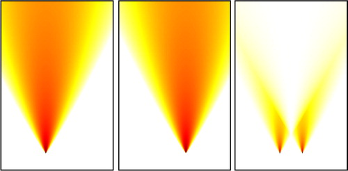
However, quite often, a simulated plume could differ from the true plume by a spatial or temporal displacement, which cannot be estimated by a local measure of discrepancy. In such circumstances, point-wise indicators usually lead to the double penalty issue. At the edge of the simulated plume, where the concentration gradient is often found to be high, concentrations might still be significant for the plume while vanishing for the truth (or verification). Vice versa, and especially if the tracer mass is roughly the same for the plume and the truth, the simulated plume is likely to vanish where the truth might still be high, leading to doubly penalise the mismatch. This yields false alarms and misses from the same error. Yet, the simulation could be highly faithful but would only suffer from a small displacement when compared to the truth. Figure 1 illustrates the double penalty effect.

Fig. 1 Illustration of the double penalty effect: a simulated Gaussian plume (left panel) where the source has been shifted to the left compared to the true Gaussian plume (middle panel). The squared difference is plotted on the right panel and it is characterised by two maxima: on the right, the simulation is penalised for not predicting the plume where it should be and on the left the simulation is penalised for predicting a plume where there is none.

In the context of an accidental release of pollutant, such displacement could be produced by a space or time shift of a point-wise source, which is a non-local error. It could also be induced by locally uncertain meteorological fields, whose errors are slowly accumulating while simulating the plume resulting in a non-local effect. This is also induced after some time by uncertain chemistry, dry deposition and wet scavenging, which are not, per se, a source of direct displacement error.

Such undesired effect has been put forward and studied in the forecast of precipitations. Via deposition, this double penalty also affects the deposition map of pollutants, whose measurement and simulation are critical for long-range transported harmful radionuclides such as iodine-131, cesium-134 and cesium-137.

1.2. Non-local metric to compare fields of pollutants

To perform verification of non-local nature, several strategies and their statistical tools have been developed. Gilleland et al. (2010a) distinguish four types of methods. The first one is scale separation which can be obtained by decomposition on an adequate function basis or frame using wavelets or analogous transformation (e.g. Briggs and Levine, 1997; Lack et al., 2010). The second is based on fuzzy methods which smooth the fields out prior to comparisons (e.g. Ebert, 2008; Amodei and Stein, 2009). The third one focuses on the identification and comparison of features of the fields, emphasising simple patterns or objects in the fields (e.g. Davis et al., 2006a, b). The fourth strategy is based on field deformation or field displacement (Hoffman et al., 1995). Methods based on optical flow techniques have been developed to that end. They can combine a multiscale analysis with a displacement matching analysis (e.g. Keil and Craig, 2007, 2009; Marzban and Sandgathe, 2010). They can be based on image warping techniques (Gilleland et al., 2010b), which amounts to identifying a set of points in the domain and images of these points by the warping transformation that would best approximate the displacement between the forecast and the verification. In the context of tracer dispersion, we observe that such deformation can indirectly be accomplished by the estimation of a field of diffusion coefficients to adapt the transport of the plume so as to better match the verification (Bocquet, 2012). To the best of the authors’ knowledge, none of these displacements methods has been directly applied to comparison of verification of simulated accidental atmospheric plumes of pollutant.

In this article, we intend to experiment on another type of measure belonging to this fourth class of methods and pertaining to the displacement: the Wasserstein distance. This metric assumes that the forecast and verification fields are densities that can be transported one into the other, in a similar way as the warping. Every transportation map (or a generalisation thereof) has a cost that measures how much work is required to move masses (Monge, 1781; Kantorovich, 1942; Villani, 2008). Then, one selects the transportation map that has the least cost. The value of the cost of this optimal transport defines the distance between both fields. As opposed to the warping methods, there is no sampling of the fields since they are considered globally. In spite of the mathematical and numerical difficulty attached to the definition and implementation of such distance, it has attracted a lot of attention in applied mathematics – in image treatment and restoration notably – because of its elegance and its connection to convex optimisation.

In this article, we apply it to the dispersion of the radionuclides in the air in the aftermath of the Fukushima-Daiichi Nuclear Power Plant (FDNPP) accident.

1.3. The Fukushima-Daiichi radionuclides atmospheric dispersion accident

On 11 March 2011, a magnitude 9.0 earthquake occurred in the Pacific about 130 km off the northeast coast of Japan. The earthquake was followed by a tsunami giving rise to the INES (International Nuclear Event Scale) level 7 accident in the FDNPP. Large amounts of radionuclides were released into the ocean and the atmosphere (Butler, 2011; Chino et al., 2011; Mathieu et al., 2012). Released radioactive nuclides were deposited in the environment over a wide area. Kawamura et al. (2011), Morino et al. (2011), Aoyama et al. (2012), Groëll et al. (2014) and others estimated that about 80 % of the atmospheric emissions were deposited in the Pacific Ocean and 20 % were deposited over Japan. The size of the contamination zone in Japan with levels greater than 185 kBq/m² covers approximately 1700 km² (Steinhauser et al., 2014). Radionuclides were mainly deposited northwest of the installation, causing the greatest contamination area (Kinoshita et al., 2011; Yasunari et al., 2011).

Environmental monitoring including air-borne survey (MEXT, 2011) and soil sampling (Saito et al., 2015b) was performed to map the deposition density of cesium on the ground surface in eastern Japan. Those data were intensively used to assess the performance of models to simulate the FDNPP accident (Morino et al., 2011; Terada et al., 2012; Korsakissok et al., 2013; Saunier et al., 2013; Draxler et al., 2015). Model-to-data, but also model-to-model comparison, showed discrepancies that highlighted the strong uncertainties that remain. The assessment of the total amount released in the atmosphere during the accident is fairly reliable, whereas the temporal evolution of the release rate for each radionuclide varies depending on the source term estimation method and the meteorological data (Stohl et al., 2012; Terada et al., 2012; Winiarek et al., 2012; Saunier et al., 2013; Winiarek et al., 2014; Katata et al., 2015). The meteorological conditions are also identified as being an important source of uncertainties (Korsakissok et al., 2013; Arnold et al., 2015; Sekiyama et al., 2015).

In these studies, the quantification of the model-to-data discrepancies is based on the classical statistical indicators initially proposed by Chang and Hanna (2004). The usual indicators proved to be inefficient to express the agreement/disagreement between simulations and observations, and there is a need to find new indicators to better express the performance of models to simulate the dispersion of an accidental release.

The Institute for Radiological Protection and Nuclear Safety (IRSN) developed a database gathering the radiological measurement data of any type from multiple sources into a single resource, ensuring the traceability of the measurement campaigns and simplifying the data mining to end users (Quérel et al., 2016). In the present work, this database is used to evaluate the mean deposition of cesium-137 on the model meshes at a given date in order to be used to quantify the model-to-data discrepancies. This end-user query has been carried out by interpolating the cesium-137 deposition data on the computational mesh, deriving arithmetic mean values that also account for radioactive decay.

1.4. Outline

In Section 2, we first provide a mathematical and conceptual introduction to the optimal transport theory, as well as the definition of the Wasserstein distance. In Section 3, building on Papadakis et al. (2014), we describe a numerical algorithm that allows to compute the optimal transport map and the related Wasserstein distance. We explain how we have extended this algorithm to account for tracer transport specifics. We also describe and point to an openly available python code of the algorithm. This is an improved and extended declination of that provided by Papadakis et al. (2014), which we refactored to be fast enough for the purposes of this study. In Section 4, we apply the technique to the comparison of simulation outputs of the Fukushima-Daiichi radionuclides atmospheric dispersion event. We study the behaviour of the Wasserstein distance compared to more standard, local statistical indicators. Finally, it is applied to the verification of a simulated deposition map with the deposition map obtained from the observations of the IRSN database. The conclusions are drawn in Section 5.

2. The Wasserstein distance

The optimal transport theory on which is based the Wasserstein distance was born in the 17^th century in a famous memoir by Gaspard Monge (Monge, 1781) and later modernised by Kantorovich (1942). Many recent contributions have been published since then on the revitalised subject (Villani, 2008, and references within). In this section, we first provide a mathematical and conceptual introduction to optimal transport and the definition of the Wasserstein distance.

2.1. Definition of the Wasserstein distance

Let us define as the set of density functions defined over the Euclidean space of dimension d, that is, that are non-negative over and which satisfy1

We will say that a map transports the density f ₀ into the density f ₁ if, for any subset in , we have2

Let us assume T to be a bijection and to be sufficiently regular (infinitely differentiable typically). We can change variable x=T(y) in the right-hand side of eq. (2) to obtain3 where Jac(T), a non-negative number, is the absolute value of the determinant of the Jacobian matrix, that is,4

Because the identity eq. (3) must be valid for all subsets since T is a transport map, eq. (2) should be equivalent on to5

In a condensed form, we write f ₁=T#f ₀, meaning that the density f ₀ is transported by T onto f ₁.

Now, we consider the space of sufficiently regular bijections that map f ₀ into f ₁, that is, those that satisfy eq. (5). One can define a cost J(T) attached to such a transport map as6 where C is a symmetric cost function defined over . It ascribes a cost C(x,y) to moving a unit mass from point x to point y in . In this article, we choose the square of the Euclidean distance defined over 7 The Wasserstein distance defined in based on the Euclidean distance in , which we will loosely call the Wasserstein distance without reference to the chosen cost in the rest of the article, is given by8

It can be mathematically proven that because this Wasserstein distance is based on the Euclidean distance, there exists a unique map T* in minimising J. Hence, the infimum is in fact a minimum, which is not always guaranteed for costs J based on other distances C (Villain, 2008). The regularity of the optimal transport map is proven in Section 7.1 of Ma et al. (2005) for this specific cost function.

We are interested in the value of the distance itself, that is, the minimum of J. We are also interested in the optimal transport map T*, the argument of the minimum, as it may tell us where the main discrepancies between the two densities are and how much mass should be displaced to match them.

2.2. The fluid mechanics formulation

Originally, Monge introduced a temporal dimension to the problem. A mass piece transported from one heap (the initial density function) to the other follows a continuous trajectory from point x in , where the mass piece originally lies, to point T(x) in . As we saw, this interpretation is not mandatory to define the distance and the optimal transport map. Nonetheless, the introduction of time offers a non-trivial interpolation between the initial and the targeted densities. It eases a physical interpretation of the optimal map. It is also a source of inspiration to design numerical algorithms to compute the optimal map and its distance (Benamou and Brenier, 2000; Papadakis et al., 2014). Finally, it is a way to demonstrate the underlying convexity of the minimisation problem which leads to the existence and unicity of the optimal map.

Following Benamou and Brenier (2000), we define as the set of couples of maps (f, v) defined over9

which satisfy the continuity constraint10

and the boundary conditions, for all x in 11

If the domain has boundaries , the condition12 should be imposed to maintain mass conservation. The variable plays the role of a fictitious time, f is a density field defined over that interpolates between f ₀ and f ₁, and v is a velocity field that advects the density field f.

We define the following cost for an interpolation13 which physically represents twice the kinetic energy of displacing f ₀ into f ₁.

As in the previous section, we define14

It can be shown that if the cost eq. (13) is seen as a function of (f, f v), that is, density and momentum, instead of (f, v), it becomes a strictly convex functional of its variables. This can be easily checked by computing the Hessian of the functional. This is useful to prove the existence and unicity of the minimisation problem eq. (14). The unique argument (f*, v*) of the minimum will then be called the optimal interpolation.

A key result is that if T* is the optimal transport map transporting f ₀ into f ₁, the density field at time t in [0,1] of the optimal interpolation between f ₀ and f ₁ is given by15 that is, for all , . Explicitly, we have16

Importantly, it can further be shown that, (f*,v*) and T* being related by eqns. (10,11,12,15),17

Hence, W _c (f _0, f ₁) coincides with the Wasserstein distance W(f _0, f ₁). Therefore, this fluid mechanics formulation of the optimal transport problem could be used as a means to numerically solve it. This result is heuristically proven in Section 3 of Benamou and Brenier (2000). Note that the optimal map follows a linear interpolation between the identity and . However, the density is interpolated in between f ₀ and f ₁ in a non-linear fashion.

Figure 2 illustrates a one-dimensional optimal transport problem defined on . The optimal transport solution is very different from the traditional linear interpolation solution.

Fig. 2 Illustration of the traditional linear interpolation (left) and of the optimal transport interpolation (right) between two normalised densities defined in the domain [0,1]. Interpreting the densities as mass distributions, the traditional linear interpolation appears as a non-physical displacement.

We now focus on a peculiar one-dimensional problem which will also be of use in our radionuclide dispersion application.

2.3. Optimal transport in one dimension

Here, we suppose that d=1 and . We define the cumulative distribution function (cdf) for , i=1,2 as18

Hence, we have and the cdfs are increasing function of x. This enables the definition of their right-inverse by19 possibly taking the values and . It can be shown that the optimal transport map from to is defined by20

and the Wasserstein distance is given by21

A heuristic derivation is given in Appendix A.

This map is often referred to as an anamorphosis (Wackernagel, 2003). Because it is defined for one-dimensional problems and not two-dimensional (and higher) problems of relevance to this study, it cannot be used directly onto the pollutant fields for d≥2. However, it can be used to define a weaker but nonetheless useful form of transport from one concentration field to another in any dimension.

2.4. Transport of concentration scales

Instead of transporting a whole field of concentrations, we focus on the definition of a palette, or grey scales, of concentrations and how to transport the palette of a concentration field into the palette of another concentration field. To do so, we need to measure the area in where a density has values in between two bounds. Hence, we define for a subset of its measure22

where is the characteristic function of which takes the value 1 for x in and the value 0 outside of .

We assume that the f _i are defined on , two compact subsets, which is a valid assumption for the environmental applications we have in mind. We can define the palette G _i for f _i by23 which is complementary to the classical notion of distribution function defined in integration theory. Specifically, G _i (x) is the normalised measure of , whose complement set is known as the -highest posterior density of f _i in Bayesian statistics.

G _i is assumed to be regular enough. It can also be seen as the cdf of the probability density function (pdf) g _i defined by24

Instead of considering the optimal transport from f ₀ to f ₁, we consider the one-dimensional optimal transport from g ₀ to g ₁. Hence, the optimal map is . Consequently, the palettes are related by or .

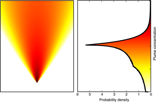
Figure 3 illustrates the palette in the case of a Gaussian plume.

Fig. 3 Gaussian plume (left) and the pdf derived from the plume colour palette (right).

3. Algorithm and code

In this section, building mostly on Papadakis et al. (2014), we will briefly describe a numerical algorithm that allows to compute the optimal transport map and the related Wasserstein distance.

3.1. Algorithm

The main idea is to compute the optimal transport map by solving the fluid dynamics optimisation problem of Section 2.2 first. This optimisation problem is a continuous optimisation problem under constraints in dimension d+1, where +1 accounts for the fictitious time dimension. One is looking for the pair (f, v) which is admissible, that is, satisfying the continuity equation eq. (10) and the boundary conditions eqs. (11) and (12), and minimising the cost function of eq. (13).

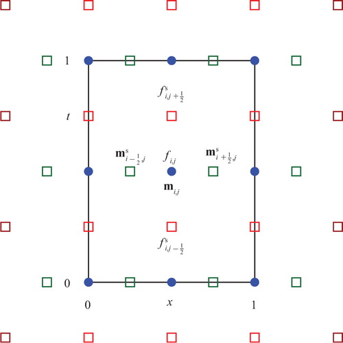
One complication is due to the numerical discretisation of this fluid dynamics problem. A numerical solution of the continuity equation requires a definition of both the density field (f) and the momentum field (m=f v) on staggered grids. This allows an accurate representation of the derivatives in the continuity equation thanks to second-order centred differences. Yet the computation of the cost function requires both fields to be defined on the same grid. One way to properly discretise these equations is to introduce the same field twice, one for each grid, and add the constraint that the two numerical representations of this unique field are connected by an interpolation operator. This adds another constraint to the optimisation problem, which requires the fields to be defined on the centered and on the staggered grids. Figure 4 illustrates the centered and staggered grids with a typical one-dimensional setup (d=1).

Fig. 4 A typical one-dimensional setup (d=1), where . The centred grid where is defined and the staggered grid where is defined are both represented (bullets and squares respectively). The reservoir variables extends the domain on the left and on the right (darker squares on the lateral boundaries of the staggered grid).

The numerical cost to be minimised F, as a function of the numerical discretisation of (f, m) on both grids, has in fact been defined as the sum of

• one term F ₁ which consists of the cost function, discretisation of eq. (13), and of a penalty term that enforces the continuity equation and the boundary conditions. For the cost function and the boundary conditions, this term further decomposes into a sum of local terms, one for each site. These terms do not mix fields on the centered and staggered grids;

• one term F ₂ which consists of the interpolation constraint between the fields defined on the two grids.

With the constraints encoded in the numerical cost function F, it can be freely minimised with respect to both copies of the discretised fields.

There exists a class of optimisation algorithms in the applied mathematics literature that are meant to minimise cost functions that are sums of several terms of different type. The terms are minimised independently (which can be parallelised), and their interdependence is enforced via the iteration of the minimisation. Under mild assumptions, in particular the fact that the terms in the cost function are convex, these algorithms are guaranteed to converge. In Papadakis et al. (2014), the independent minimisations are performed using the so-called proximal operators that are generalisation of the gradient descent method. The proximal operators are also well adapted to the terms that enforce linear constraints such as the continuity equation. In that case, they coincide with projection operators onto the constraint set.

Several of these methods are advocated in Papadakis et al. (2014): the Douglas-Rachford solver (DR; Lions and Mercier, 1979), the Primal-Dual solver (PD; Chambolle and Pock, 2011), and the ADMM solver (Gabay and Mercier, 1976) meant to solve the original optimisation problem of Benamou and Brenier (2000). We tested the DR and PD solvers and looked for the fastest scheme to convergence. In agreement with Papadakis et al. (2014), we found the Primal-Dual solver to be the most efficient for our practical problem: the number of required iterations is smaller and the time taken by each iteration too. Nevertheless, we will also use the Douglas-Rachford solver as it offers a greater flexibility than the Primal-Dual algorithm (Pustelnik et al., 2011), which we shall use when adding constraints imposed by the potential absence of mass conservation. Hence, we will rely on both solvers, DR and PD, in the rest of this article.

The continuity equation constraint and the boundary conditions enforced in F ₁ are solved by a proximal operator, that is, a projection. This requires inverting linear systems for the continuity equations and its boundary conditions. We use a multiple dimension cosine fast Fourier transform (FFT) to solve this system. The constraint in F ₂ due to the interpolation operator from one grid to the staggered one is also solved using a projection. This can be solved using the inversion of a tridiagonal system whose complexity scales linearly with the size of the system.

As a result, the typical computational complexity per iteration of either our implementation of the DR or of the PD solver is , where N is number of grid cells along one spatial dimensional or along the fictitious time dimension (which could be nonetheless chosen differently from the space size). That is why such numerical solution of the optimal transport problem is costly. We will later observe that, in practice, the number of required iterations to convergence can be very significant but that an estimate of the Wasserstein distance can be nonetheless obtained with a much more limited number of iterations.

3.2. Mass conservation

As opposed to the physics and chemistry of radionuclides in the atmosphere, the optimal transport that we described so far conserves mass (of one species) as imposed by eq. (1). On short time scales, radionuclides are approximately conserved even in the presence of sources and sinks. However, we need to compare plumes with source terms that could significantly differ so that, in that case, mass conservation is unrealistic. To apply optimal transportation, we need both and to satisfy eq. (1), or at least the sufficient condition25

The simplest approach to this issue is to normalise the fields by their respective mass26

This approach focuses on the field variations and mass displacement but ignores the mass losses and injections.

We will also be interested in the fields so as to emphasise the many scales in a plume of pollutant rather than only the peaks, which requires to define a threshold of concentration f _thr below which the value is irrelevant. For these transformed fields, max(log(f _i /f _thr ),0), one cannot guarantee that their integrals coincide even if the mass is physically conserved.

Another solution consists in changing the boundary conditions on . Instead of imposing null flux conditions, we add a reservoir field defined on the domain boundary . For instance, considering a one-dimensional problem d=1 with , we would add a space variable at x=0 and one at x=1 as shown in Fig. 4. We assume that27

In case the opposite is true, we could exchange the role of f ₀ and f ₁ due to the reversibility of optimal transport (see Appendix B). At t=0 the reservoir variables that lie on the boundary are set to zero (empty reservoir) so that the total mass in the domain is . The target density at t=1 will coincide with f ₁ on and the mass contained in the reservoir on will be imposed to be δM.

This represents another constraint in the optimisation method, that can be added as a third term F ₃ in the cost function and which we have implemented using the DR solver following Pustelnik et al. (2011). For this optimal transport problem with specific boundary conditions, it would be desirable to confirm the existence, the uniqueness and the regularity of the solutions e.g. using the MTW conditions (Ma et al., 2005). However, this should not be an easy task since the final density is a distribution rather than a bounded regular function.

3.3. Code

All the schemes used in the algorithm rely heavily on basic linear algebra routines and on variants of the FFT. Those are handled well and efficiently by the python language. Our code was initially inspired by the MATLAB^® code (github.com/gpeyre/2013-SIIMS-ot-splitting) but later diverged significantly in terms of optimisation and new functionalities. Our python code is object-oriented and rely on several standard scipy library modules: scipy.fftpack, scipy.interpolate, scipy.integrate and numpy: numpy.linalg, numpy.meshgrid, numpy.tensordot, etc. that considerably accelerate the main algorithmic operations.

The code is not parallelised and run on a single CPU core. Most of the main steps of the algorithms could actually be parallelised to deal with higher dimensional spaces. As an indication, we give in Table 1 the wall-clock time taken to run 10³ iterations of the DR and PD solvers for a d=1 and a d=2 optimal transport problems for several resolutions, using our code. The test is run on a single core of an Intel processor i5 at 2.5 GHz. As expected from the complexity analysis, these times scale roughly linearly with the problem size.

Table 1. Wall-clock time spent in seconds on 10³ iterations of several optimal transport problems in d=1 and d=2 for the DR and PD solvers and for several resolutions

d=1			d=2
Resolution	DR	PD	Resolution	DR	PD
32^2	1.4	1.1	32^3	31.2	23.8
64^2	3.0	2.6	64^3	295.5	258.0
128^2	13.7	11.1	128^3	2970.5	2420.6

The code is available at cerea.enpc.fr/opttrans/.

4. Application to the Fukushima-Daiichi event

We apply the Wasserstein distance to several examples of model-to-model and model-to-data comparisons in the context of the atmospheric dispersion of cesium-137 from the FDNPP in March 2011.

4.1. Setup

We use the same model setup as in Winiarek et al. (2014). In particular the Polyphemus chemical transport model (Quélo et al., 2007) is run over a 120×120 grid of resolution 0.05°×0.05° and 15 vertical levels. The meteorological fields as well as the parameterisations used in the model, such as transport, wet and dry deposition, are described in Winiarek et al. (2014). We use the source term for cesium-137 estimated in Section 3.4 of the same article, as in Quérel et al. (2016).

Our optimal transport code can handle 1D and 2D fields. Hence, the 4D simulations of the radionuclides plumes, 3D in space plus the (real) time dimension, need to be projected onto a space of lower dimension. We have considered: (1) the activity concentrations at ground level and fixed time, with a threshold of 10⁻³ Bq.m⁻³, (2) the activity concentration averaged over the air columns at fixed time with a threshold of 10⁻⁵ Bq.m⁻³, (3) the deposition map of cesium-137 on the ground with a threshold of 10⁴ Bq.m⁻². A threshold is used whenever the logarithm of the activity concentrations is considered rather than the raw concentrations defined in linear scale.

4.2. Model-to-model comparisons

In order to emulate model error and to create situations where the double penalty effect applies, we perturb the simulation of Winiarek et al. (2014) by displacing the source term in space and in time. More precisely, we have considered nine simulations of the cesium-137 plume that differ by the position in space of the source and by the starting date of the same source term. Simulation with number k=3×i+j, has a source location shifted by −1, 0, 1 degree in longitude depending on i=0, 1, 2 respectively, and has a source term shifted in time by −3, 0, 3 hours depending on j=0, 1, 2 respectively. That makes 36 distinct simulation pairs where a comparison can be performed.

For the systematic study of all pairs, we either degrade the simulation resolution to 0.2°×0.2° on a 30×30 grid so that the related continuous optimal transport has coarse resolution 30³, or use the simulation grid 120×120, with a related continuous optimal transport that has high resolution 120²×30. The coarse resolution experiments are considered because they exhibit a much faster convergence.

We use the PD optimisation method when the concentration fields to be compared are normalised to 1 and we use the DR optimisation method when the reservoir method is used instead to avoid normalisation of the fields. Also note that even with the DR optimisation method, the fields are normalised by the total mass of one simulation, typically the simulation that predicts the largest mass. Hence, we compare the two-dimensional pdf of dimensionless fields and the Wasserstein distance has the dimension of a distance.

We focus on the cesium-137 activity concentrations at ground level at 7:00 UTC on 25 March 2011 – during the release of a pollutant plume – using the logarithm of the concentrations for a stronger contrast (see Fig. 5). In Fig. 6, we consider each pair of simulation. We compute the Pearson correlation coefficient, the mean square error, the Wasserstein distance using normalisation or the reservoir approach, for both coarse and high resolutions.

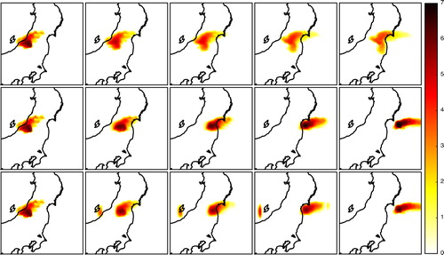
Fig. 5 Cesium-137 activity concentration at ground level at 7:00 UTC on 25 March 2011. The concentrations values are displayed in logarithmic scale using max(log₁₀(c/c _thr),0), where c is the activity concentration and c _thr=10⁻³ Bq.m⁻³ is the threshold. The plot of the simulation indexed by 3×i+j is shown in row i and in column j. Hence, simulations in the same row have the same source location and simulations in the same column have the same time shift.

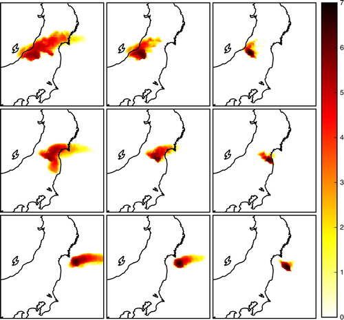
Fig. 6 Tables of indicators between two simulations. The mean square error (MSE) and the Pearson correlation coefficient (PCC) are displayed in the first column. The Wasserstein distance using the normalisation method W_n , using high resolution (hr) or coarse resolution (cr) is displayed in the second column. The Wasserstein distance using the reservoir method W_r , using high resolution (hr) or coarse resolution (cr) is displayed in the third column. The darker shades correspond to the highest matches (smallest values for the mean square error and the Wasserstein distance, and highest values for the correlation) and the dimmer shades correspond to the lowest matches (highest values for the mean square error and the Wasserstein distance, and smallest values for the correlation). The cell in the k-th row and l-th column compares simulation k to simulation l following to the simulation numbering described in Fig. 5.

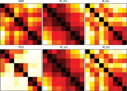
The correlation tends to discriminate the simulations with distinct space shifts. This is supported by the computation of the main empirical orthogonal functions of the matrix of the correlation coefficients where the simulations with different spatial shift are seen to be dominant. The simulations that are similar according to the mean square error indicator are those with the same space shift and adjacent time shift. This is due to the fact that adjacent simulations have much bigger overlap region for the cesium-137 plume than non-adjacent simulations. This is a consequence of the relatively large space and time shifts we chose for the source. As opposed to the correlation and mean square error, the Wasserstein distance is much less discriminating. The permissiveness of the Wasserstein distance was expected and hoped for since it is meant to avoid the double penalty effect. However, it does discriminate simulations with different space shifts of the source location in the normalisation approach case, and simulations with distinct time shifts in the reservoir approach case. By contrast, the Wasserstein distance in the reservoir approach seems more discriminating than in the normalisation case as can been seen in Fig. 6. When computing the optimal interpolation and the associated cost, one expect the Wasserstein distance to be the sum of the cost of a long-range transport and the cost of small-range reorganisations. In this study, because of the relatively large shift, the cost of the long-range transport is greater than the cost of the reorganisation, which explains the behaviour of the Wasserstein distance with normalisation. Then, one remarks that, due to the relatively long time shift and the specific time chosen, the time shift greatly influences the total mass of pollutant on the map. Indeed, since we chose an instant during the release of a pollutant plume, simulations whose source term is delayed necessarily carry a lower mass of pollutant. Hence, when computing the optimal interpolation between two maps with different time shifts, most of the associated Wasserstein distance is ascribed to moving the extra mass into the reservoirs, which are very far. This explains the behaviour of the Wasserstein distance with reservoirs.

Fig. 7 Illustration of the deformation induced by optimal transport of cesium-137 plumes at ground level at 7:00 UTC on 25 March 2011, between simulations 1 and 3 using normalisation (top panels), between simulations 1 and 6 using normalisation (middle panels), and simulations 1 and 6 using the reservoir technique (bottom panels). The deformation of the plumes are shown at five time steps, the first one being the concentration field of the first simulation, and the last one being the concentration field of the second simulation. The concentrations values are displayed in logarithmic scale using max(log₁₀(c/c _thr),0), where c is the activity concentration and c _thr=10⁻³ Bq.m⁻³ is the threshold.

Moreover, we observe that the Wasserstein distance values in the coarse resolution case are quite close to the values of the Wasserstein distance in the high resolution case. Since the long-range transport dominates the small-range reorganisations in the Wasserstein distance, and because even a coarse resolution can capture the shape of long range transport, this was expected. This indicates that the cost of computing the Wasserstein distance between fields could be considerably alleviated by downgrading the resolution of the fields.

The use of the continuous optimal transport is illustrated in the high resolution case in Fig. 7, using the normalisation approach in two instances, and using the reservoir approach in a third instance.

Fig. 8 Concentration histograms of simulation 4, 6 and 8. The concentrations values are in logarithmic scale using max(log₁₀(c/c _thr),0), where c is the activity concentration and c _thr=10⁻³ Bq.m⁻³ is the threshold.

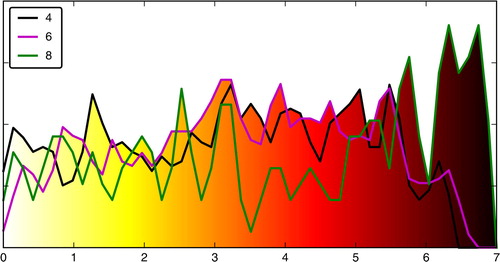
Following our presentation of the optimal transport in dimension one in Section 2.3, we illustrate the use of the Wasserstein distance and the optimal transport between concentration histograms of three simulations. We have chosen to focus on simulations 4, 6 and 8 (see Fig. 5). Their activity concentration histograms are shown in Fig. 8 and the indicators between these simulations are reported in Table 2.

Table 2. Table of statistical indicators between simulations 4, 6 and 8: the Wasserstein distance using normalisation (W_n ), the Wasserstein distance using reservoirs (W_r ), the Wasserstein distance between the colour palettes (W_p ), the mean square error (MSE) and the Pearson correlation coefficient (PCC)

	W n [km]	W r [km]	W p	MSE	PCC
4 vs 6	4.47	3.84	0.0383	1.04	−0.03
4 vs 8	2.46	5.90	0.698	0.69	−0.02
6 vs 8	1.11	1.40	0.544	0.56	0.32

For these situations, the Wasserstein distance behaves similarly to the statistical indicators: the best match is found for simulations 6 and 8. This is a consequence of the big overlap region between these simulations (they share the same spatial position of the source). However, when looking at the maps on Fig. 5, simulations 4 and 6 look subjectively very similar and are quite different from simulation 8. Indeed, simulations 4 and 6 are characterised by a high activity concentration near the position of the source, which seems to have been advected eastward by the wind, whereas this advected pattern is absent in simulation 8. This is objectively confirmed when looking at the histograms of Fig. 8: the colour palette for simulation 8 is much higher in the highest concentration values than both palettes for simulations 4 and 6. This latter characteristic mostly impacts the Wasserstein distance between the colour palettes (W_p ), hence the very small distance between 4 and 6. This shows that this quick-to-compute Wasserstein distance could be used as a reliable indicator to identify matches between patterns of the plumes.

4.3. Comparison to deposition data

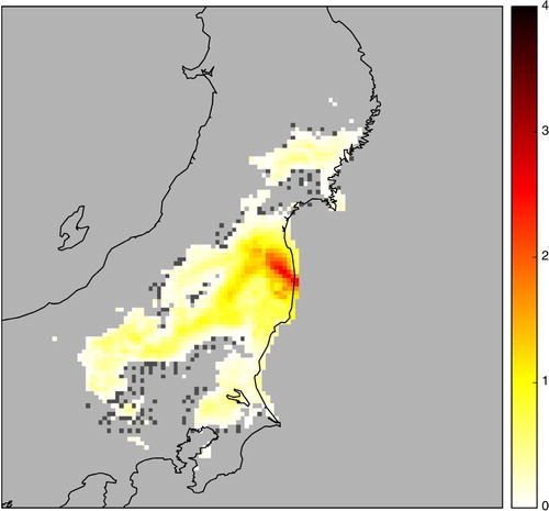
As mentioned in the introduction, a cesium-137 activity deposition map has been extracted from the observation database of IRSN. These observations were obtained from airborne campaigns (Sanada et al., 2014) and soil sampling campaigns (Endo et al., 2012; Saito et al., 2015b). This map is shown in Fig. 9 using deposition values in logarithmic scale.

Fig. 9 Observations of the cesium-137 activity deposited on the ground in logarithmic scale max(log₁₀(c/c _thr),0), where c is the activity concentration and c _thr=10⁴ Bq.m⁻² is the threshold. The dark grey pixels correspond to grid cells where the deposition value is known but lower than c _thr. The light grey pixels correspond to grid cells where the deposition value is below the limit of detection.

Five simulations have been performed with several models and setups and possibly distinct source terms. The first simulation follows the setup of Winiarek et al. (2014) and is denoted Winiarek et al. in the following. The source term is partially based on the assimilation of observations. The other four simulations are taken from Quérel et al. (2016) and are named IRSN 1 to IRSN 4. These simulations were chosen because of their wide range of behaviour with significantly different deposition patterns, with the goal to better characterise the behaviour of the Wasserstein distance. Our reference simulation inspired from Winiarek et al. (2014) complements this simulation ensemble. Configuration key parameterisations are given in Table 3. The corresponding cesium-137 deposition maps have been computed. They are displayed in Fig. 10 where a mask has been applied to set all simulated deposition values to zero wherever an observation is not available or lower than 10⁴ Bq.m⁻².

Fig. 10 Masked deposition maps of the cesium-137 activity in logarithmic scale max(log₁₀(c/c _thr),0), where c is the activity concentration and c _thr=10⁴ Bq.m⁻² is the threshold for the observations, and five model simulations.

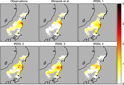
Table 3. Configuration setups for the four simulations from Quérel et al. (2016)

Simulation	Rain	Source term	Granulometry
IRSN 1	WRF (Winiarek et al., 2014)	Saunier et al., 2013	1982; maritime
IRSN 2	radar (Saito et al., 2015a)	Saunier et al., 2013	Jaenicke, 1982; urban
IRSN 3	WRF (Winiarek et al., 2014)	Saunier et al., 2013	Jaenicke, 1982; continental
IRSN 4	radar (Saito et al., 2015a)	Saunier et al., 2013	Jaenicke, 1982; urban
Simulation	Wet deposition velocity	In-cloud scavenging	Below-cloud scavenging
IRSN 1	(Zhang et al., 2001)	1991	Neglected
IRSN 2	(Zhang et al., 2001)	1999	Quérel et al., 2014, and Blanchard, 1953
IRSN 3	0.2 cm·s^−1	Roselle and Binkowski, 1999	IRSN model
IRSN 4	0.2 cm·s^−1	Neglected	Laakso et al., 2003

We have also considered zoomed deposition maps in the region where most of the deposited activity lies. They are shown in Fig. 11. In this region, it is interesting to use verification using linear scale depositions because the fields are not as multiscale as in the large scale maps.

Fig. 11 Zoomed masked deposition maps of the cesium-137 activity in logarithmic scale max(log₁₀(c/c _thr),0), where c is the activity concentration and c _thr=10⁴ Bq.m⁻² is the threshold for the observations, and five model simulations.

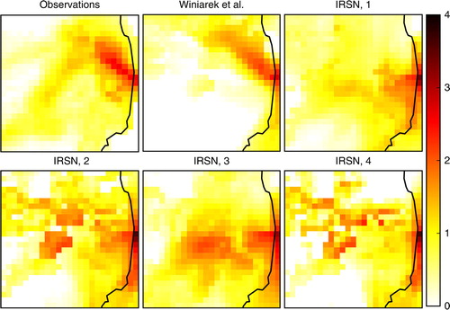
In the context of this verification to deposition data, the reservoir approach is not physical. Penalising the extra mass by moving it to the boundary does not match any physical mass motion. Removing activity from the ground to help match two maps should not involve lateral boundary conditions as opposed to the same problem with radioactive plumes. The mean squared error (MSE), the Pearson correlation coefficient (PCC), and the Wasserstein distance (W) have been computed for the five simulations. Also note that, in order to allow a fair comparison of the large scale maps, all indicators have been computed by applying a filter to mask all data in the area where observed deposition is lower than c _thr=10⁴ Bq.m⁻². We did not apply this filter for the zoomed map since only a few grid cells would have been affected. The results are reported in Table 4 for the large scale maps using a logarithmic scale and for the zoomed maps using a linear scale.

Table 4. Mean squared error (MSE), Pearson correlation coefficient (PCC) and Wasserstein distance (W) of the comparison between the deposition values of one of the five simulations and the observation values, for the whole map of the zoomed region where most of the deposited activity lies

	large scale, logarithmic scale			zoom, linear scale
Simulation	MSE	PCC	W [km]	MSE [×10^6 Bq.m^−2]	PCC	W [km]
Winiarek et al.	0.017	0.73	69.0	0.522	0.76	20.1
IRSN 1	0.020	0.77	24.1	7.72	0.40	39.1
IRSN 2	0.023	0.78	28.8	18.0	0.39	38.3
IRSN 3	0.026	0.79	30.0	3.79	0.41	43.2
IRSN 4	0.024	0.69	36.0	20.8	0.37	41.3

With the linear scale, the simulation Winiarek et al. obtains the best MSE and PCC which is not a surprise since it is driven by a source term that has been obtained by inverse modelling using an MSE-like criterion. The Wasserstein distance consistently follows this trend and ranks the simulations in the same order as the MSE but in a smoother fashion because the double penalty of the MSE indicator is avoided. With the logarithmic scale, the Winiarek et al. simulation still has the best MSE, but it has the worst Wasserstein distance to the observation map. We have checked that this simulation is penalised by the western branch of the deposition pattern in the Nakadori Valley which is barely represented in the Winiarek et al. simulation. This branch is hard to simulate because it is highly dependent on meteorological and orographical effects. It is also penalised by the absence of significant deposition south and west of the Nakadori Valley. Hence, activity must be transported to match the observation pattern which has a significant cost. Differently, even if this branch is incorrectly represented, the other simulations do predict more significant activity deposited in this area, which can be transported in the optimal transport and yield a lower Wasserstein distance. This characteristic of the Wasserstein distance was hoped for. We observe that it can lead to a quite different conclusion than the MSE which could be dominated by activity peaks.

5. Conclusion

In this article, we have illustrated the use of the Wasserstein distance as a field-displacement-based indicator in order to compare fields of pollutants in the context of the radionuclide atmospheric release of the FDNPP accident. The Wasserstein distance was computed by solving the optimal transport problem in its fluid mechanics formulation, using proximal splitting algorithms such as the Primal-Dual algorithm and the Douglas-Rachford algorithm. In order to cope with situations where the mass is not conserved, we introduced two different approaches: the first one simply consists in normalising the fields whereas the second one expands the domain with reservoirs.

We use the Wasserstein distance as well as traditional statistical indicators to compare couples of simulations of the accidental cesium-137 dispersion, but also to verify five simulations against an observed cesium-137 deposition map. In these examples, the Wasserstein distance behaves similarly to the traditional statistical indicators but seems to be less discriminating, which was expected as a consequence of the removal of the double penalty effect. We remarked and explained differences between the method using normalisation and the one using reservoirs. We observe that using the Wasserstein distance, the long-range transport cost dominates the small reorganisation cost. This enabled us to use coarse resolution to rapidly estimate the Wasserstein distance. Nevertheless, we also showed that the choice of the quantity scales (linear or logarithmic) remains critical in the context of atmospheric dispersion due to the many scales involved.

Finally, we also proposed to compute the Wasserstein distance between colour palettes, that we found to be a quick-to-compute and reliable indicator to match specific patterns in the fields.

The reservoir method we used in this study is a rather adhoc method constructed for the purpose of this study. Contrary to the simple but raw normalisation method, the information about the total mass of the pollutant plume is not lost. However, in some specific situations, the cost assigned to moving the mass excess to the reservoir is very high, leading to dramatically different values of the Wasserstein distance. Moreover, in some cases, one can doubt the physical meaning of the method. This approach could be improved. For instance, an extra reservoir variable representing soil could be attached to each space variable rather than only at the lateral boundaries. A substantial cost would be assign to moving masses to these new reservoir variables. This would account for the physical loss processes in the comparison of fields. This would require an extension of the mathematical technique, which is in principle feasible.

Finally, the algorithms we presented in this article could be parallelised. This implies that the method could be used with higher resolution or with more than two dimensions, allowing us to compare three-dimensional fields or even four-dimensional trajectories. Also note that these methods, that we used in the context of atmospheric dispersion, can be applied to other fields in geophysics, like for example meteorology, climate sciences, where field-displacement verification techniques are valuable tools.

6. Acknowledgements

The authors thank Arthur Vidard for sharing his expertise and pointing out to us the work of Papadakis et al. (2014). The authors are grateful to two anonymous reviewers for their comments and suggestions that helped improve the article.

7. Appendix

7.1. Appendix A: One-dimensional optimal transport and anamorphosis

We consider the transport in dimension one defined by the cost eq. (7) and deterministic transport maps that transport f ₀ into f ₁, and where is a closed interval of ℝ. Using the right-inverse eq. (19) of the cdfs eq. (18), we define a generic map which is assumed to be sufficiently regularA1 where h is differentiable map from [0,1] to [0,1]. Let us see under which condition T _h transports f ₀ into f ₁, that is, if T _h satisfies eq. (5). We haveA2

For eq. (5) to be satisfied, we need over 𝔼 or over [0,1]. Hence h is the identity over [0,1], so that under sufficiently regular conditions, the only admissible transport map isA3

Moreover, we haveA4 which yields eq. (21).

7.2. Appendix B: Reversibility of optimal transport

The optimal transport is reversible in time. The property is desirable and has been checked numerically in our experiments.

Let us first show that the optimal map T _0:1 that transports f ₁ to f ₀ is the inverse of the optimal map T _1:0 that transports f ₀ to f ₁. For any map T in , we can make the change of variable y=T(x) in eq. (6)B1 which implies that by the unicity of the optimal transport map.

Next, we can rewrite the optimal map that transports , rather than , to and obtainB2

To summarise, we have the reversibility relationshipB3 whereB4

References

- Amodei M., Stein J. Deterministic and fuzzy verification methods for a hierarchy of numerical models. Meteorol. Appl. 2009; 16: 191–203. DOI: http://dx.doi.org/10.1002/met.101.
- Aoyama M., Tsumune D., Uematsu M., Kondo F., Hamajima Y. Temporal variation of 134Cs and 137Cs activities in surface water at stations along the coastline near the Fukushima Dai-ichi Nuclear Power Plant accident site, Japan. Geochem. J. 2012; 46: 321–325. DOI: http://dx.doi.org/10.2343/geochemj.2.0211.
- Arnold D., Maurer C., Wotawa G., Draxler R., Saito K., co-authors. Influence of the meteorological input on the atmospheric transport modelling with FLEXPART of radionuclides from the Fukushima Daiichi nuclear accident. J. Environ. Radioact. 2015; 139: 212–225. DOI: http://dx.doi.org/10.1016/j.jenvrad.2014.02.013.
- Benamou J.-D., Brenier Y. A computational fluid mechanics solution to the Monge-Kantorovich mass transfer problem. Numer. Math. 2000; 84: 375–393. DOI: http://dx.doi.org/10.1007/s002110050002.
- Blanchard D. C. Raindrop size distribution in hawaiian rains. J. Meteorol. 1953; 10: 457–473. DOI: http://dx.doi.org/10.1175/1520-0469(1953)010<0457:RSDIHR>2.0.CO;2.
- Bocquet M. Parameter field estimation for atmospheric dispersion: application to the Chernobyl accident using 4D-Var. Q. J. Roy. Meteorol. Soc. 2012; 138: 664–681. DOI: http://dx.doi.org/10.1002/qj.961.
- Briggs W. M., Levine R. A. Wavelets and field forecast verification. Mon. Wea. Rev. 1997; 125: 1329–1341. DOI: http://dx.doi.org/10.1175/1520-0493(1997)125<1329:WAFFV>2.0.CO;2.
- Butler D. Radioactivity spreads in Japan. Nat. News. 2011; 471: 555–556. DOI: http://dx.doi.org/10.1038/471555a.
- Chambolle A., Pock T. A first-order primal-dual algorithm for convex problems with applications to imaging. J. Math. Imag. Vis. 2011; 40: 120–145. DOI: http://dx.doi.org/10.1007/s10851-010-0251-1.
- Chang J. C., Hanna S. R. Air quality model performance evaluation. Meteorol. Atmos. Phys. 2004; 87: 167–196. DOI: http://dx.doi.org/10.1007/s00703-003-0070-7.
- Chino M., Nakayama H., Nagai H., Terada H., Katata G., co-authors. Preliminary estimation of release amounts of 131I and 137Cs accidentally discharged from the Fukushima Daiichi nuclear power plant into the atmosphere. J. Nucl. Sci. Technol. 2011; 48: 1129–1134. DOI: http://dx.doi.org/10.1080/18811248.2011.9711799.
- Davis C., Brown B., Bullock R. Object-based verification of precipitation forecasts. Part I: methodology and application to mesoscale rain areas. Mon. Wea. Rev. 2006a; 134: 1772–1784. DOI: http://dx.doi.org/10.1175/MWR3145.1.
- Davis C., Brown B., Bullock R. Object-based verification of precipitation forecasts. Part II: application to convective rain systems. Mon. Wea. Rev. 2006b; 134: 1785–1795. DOI: http://dx.doi.org/10.1175/MWR3146.1.
- Draxler R., Arnold D., Chino M., Galmarini S., Hort M., co-authors. World Meteorological Organization's model simulations of the radionuclide dispersion and deposition from the Fukushima Daiichi nuclear power plant accident. J. Environ. Radioact. 2015; 139: 172–184. DOI: http://dx.doi.org/10.1016/j.jenvrad.2013.09.014.
- Ebert E. E. Fuzzy verification of high-resolution gridded forecasts: a review and proposed framework. Meteorol. Appl. 2008; 15: 51–64. DOI: http://dx.doi.org/10.1002/met.25.
- Endo S., Kimura S., Takatsuji T., Nanasawa K., Imanaka T., co-authors. Measurement of soil contamination by radionuclides due to the Fukushima Dai-ichi nuclear power plant accident and associated estimated cumulative external dose estimation. J. Environ. Radioact. 2012; 111: 18–27. DOI: http://dx.doi.org/10.1016/j.jenvrad.2011.11.006.
- Gabay D., Mercier B. A dual algorithm for the solution of nonlinear variational problems via finite element approximation. Comput. Math. Appl. 1976; 2: 17–40. DOI: http://dx.doi.org/10.1016/0898-1221(76)90003-1.
- Gilleland E., Ahijevych D. A., Brown B. G., Ebert E. E. Verifying forecasts spatially. Bull. Am. Meteorol. Soc. 2010a; 91: 1365–1373. DOI: http://dx.doi.org/10.1175/2010BAMS2819.1.
- Gilleland E., Lindström J., Lindgren F. Analyzing the image warp forecast verification method on precipitation fields from the ICP. Weather Forecast. 2010b; 25: 1249–1262. DOI: http://dx.doi.org/10.1175/2010WAF2222365.1.
- Gröell J., Quélo D., Mathieu A. Sensitivity analysis of the modelled deposition of 137Cs on the Japanese land following the Fukushima accident. Int. J. Environ. Pollut. 2014; 55: 67–75. DOI: http://dx.doi.org/10.1504/ijep.2014.065906.
- Hoffman R. N., Liu Z., Louis J.-F., Grassoti C. Distortion representation of forecast errors. Mon. Wea. Rev. 1995; 123: 2758–2770. DOI: http://dx.doi.org/10.1175/1520-0493(1995)123<2758:DROFE>2.0.CO;2.
- Jaenicke R.Georgii H. W., Jaeschke W. Physical aspects of the atmospheric aerosol. Chemistry of the Unpolluted and Polluted Troposphere: Proceedings of the NATO Advanced Study Institute held on the Island of Corfu . 1982; Springer Netherlands.341–373. Greece, September 28–October 10, 1981 DOI: http://dx.doi.org/10.1007/978-94-009-7918-5_14.
- Jylhä K. Empirical scavenging coefficients of radioactive substances released from Chernobyl. Atmos. Env. 1991; 25A: 263–270. DOI: http://dx.doi.org/10.1016/0960-1686(91)90297-K.
- Kantorovich L. V . On the translocation of masses. Dokl. Akad. Nauk SSSR. 1942; 37: 199–201.
- Katata G., Chino M., Kobayashi T., Terada H., Ota M., co-authors.Detailed source term estimation of the atmospheric release for the Fukushima Daiichi Nuclear Power Station accident by coupling simulations of an atmospheric dispersion model with an improved deposition scheme and oceanic dispersion model. Atmos. Chem. Phys. 2015; 15: 1029–1070. DOI: http://dx.doi.org/10.5194/acp-15-1029-2015.
- Kawamura H., Kobayashi T., Furuno A., In T., Ishikawa Y., co-authors. Preliminary numerical experiments on oceanic dispersion of 131I and 137Cs discharged into the ocean because of the Fukushima Daiichi Nuclear Power Plant Disaster. J. Nucl. Sci. Technol. 2011; 48: 1349–1356. DOI: http://dx.doi.org/10.1080/18811248.2011.9711826.
- Keil C., Craig G. C. A displacement-based error measure applied in a regional ensemble forecasting system. Mon. Wea. Rev. 2007; 135: 3248–3259. DOI: http://dx.doi.org/10.1175/MWR3457.1.
- Keil C., Craig G. C. A displacement and amplitude score employing an optical flow technique. Weather Forecast. 2009; 24: 1297–1308. DOI: http://dx.doi.org/10.1175/2009WAF2222247.1.
- Kinoshita N., Sueki K., Sasa K., Kitagawa J., Ikarashi S., co-authors. Assessment of individual radionuclide distributions from the Fukushima nuclear accident covering central-east Japan. Proc. Natl. Acad. Sci. U.S.A. 2011; 108: 19526–19529. DOI: http://dx.doi.org/10.1073/pnas.1111724108.
- Korsakissok I., Mathieu A., Didier D. Atmospheric dispersion and ground deposition induced by the Fukushima Nuclear Power Plant accident: a local-scale simulation and sensitivity study. Atmos. Env. 2013; 70: 267–279. DOI: http://dx.doi.org/10.1016/j.atmosenv.2013.01.002.
- Laakso L., Grönholm T., Rannik Ü., Kosmale M., Fielder V., co-authors. Ultrafine particle scavenging coefficients calculated from 6 years field measurements. Atmos. Environ. 2003; 37: 3605–3613. DOI: http://dx.doi.org/10.1016/S1352-2310(03)00326-1.
- Lack S. A., Limpert G. L., Fox N. I. An object-oriented multiscale verification scheme. Weather Forecast. 2010; 25: 79–92. DOI: http://dx.doi.org/10.1175/2009WAF2222245.1.
- Lions P.-L., Mercier B. Splitting algorithms for the sum of two nonlinear operators. SIAM J. Numer. Anal. 1979; 16: 964–979. DOI: http://dx.doi.org/10.1137/0716071.
- Ma X.-N., Trudinger N. S., Wang X.-J. Regularity of potential functions of the optimal transportation problem. Arch. Rat. Mech. Anal. 2005; 177: 151–183. DOI: http://dx.doi.org/10.1007/s00205-005-0362-9.
- Marzban C., Sandgathe S. Optical flow for verification. Weather Forecast. 2010; 25: 1479–1494. DOI: http://dx.doi.org/10.1175/2010WAF2222351.1.
- Mathieu A., Korsakissok I., Quélo D., Gröell J., Tombette M., co-authors. Atmospheric dispersion and deposition of radionuclides from the Fukushima Daiichi nuclear power plant accident. Elements. 2012; 8: 195–200. DOI: http://dx.doi.org/10.2113/gselements.8.3.195.
- MEXT (Ministry of Education, Culture, Sports, Science and Technology). Results of the fourth airborne monitoring survey by MEXT. 2011. Online at: http://radioactivity.nsr.go.jp/en/contents/4000/3179/24/1270_1216.pdf.
- Monge G . Mémoire sur la théorie des déblais et des remblais. 1781; 666–704. Académie royale des sciences, Paris.
- Morino Y., Ohara T., Nishizawa M. Atmospheric behavior, deposition, and budget of radioactive materials from the Fukushima Daiichi nuclear power plant in March 2011. Geophys. Res. Lett. 2011; 38: L00G11. DOI: http://dx.doi.org/10.1029/2011GL048689.
- Mosca S., Graziani G., Klug W., Bellasio R., Bianconi R. A statistical methodology for evaluation of long-range dispersion models: An application to the ETEX exercise. Atmos. Environ. 1998; 32: 4307–4324. DOI: http://dx.doi.org/10.1016/S1352-2310(98)00179-4.
- Papadakis N., Peyré G., Oudet E. Optimal transport with proximal splitting. SIAM J. Imag. Sci. 2014; 7: 212–238. DOI: http://dx.doi.org/10.1137/130920058.
- Pustelnik N., Chaux C., Pesquet J.-C. Parallel proximal algorithm for image restoration using hybrid regularization. IEEE Trans. Image Process. 2011; 20: 2450–2462. DOI: http://dx.doi.org/10.1109/TIP.2011.2128335.
- Quélo D., Krysta M., Bocquet M., Isnard O., Minier Y., co-authors. Validation of the Polyphemus platform on the ETEX, Chernobyl and Algeciras cases. Atmos. Environ. 2007; 41: 5300–5315. DOI: http://dx.doi.org/10.1016/j.atmosenv.2007.02.035.
- Quérel A., Lemaitre P., Monier M., Porcheron E., Flossmann A. I., co-authors. An experiment to measure raindrop collection efficiencies: influence of rear capture. Atmos. Meas. Tech. 2014; 7: 1321–1330. DOI: http://dx.doi.org/10.5194/amt-7-1321-2014.
- Quérel A. , Roustan Y. , Quélo D. , Benoit J.-P . Hints to discriminate the choice of wet deposition models applied to an accidental radioactive release. Int. J. Environ. Pollut. 2016; 58: 268–279.
- Roselle S. J. , Binkowski F. S . Byun D. W. , Ching J. K. S . Cloud dynamics and chemistry. Science Algorithms of the EPA Models-3 Community Multiscale Air Quality Modeling System. 1999; U.S. Environmental Protection Agency. Washington, DC, USA, EPA/600/R–99/030.
- Saito K., Shimbori T., Draxler R. JMA's regional atmospheric transport model calculations for the WMO technical task team on meteorological analyses for Fukushima Daiichi Nuclear Power Plant accident. J. Environ. Radioact. 2015a; 139: 185–199. DOI: http://dx.doi.org/10.1016/j.jenvrad.2014.02.007.
- Saito K., Tanihata I., Fujiwara M., Saito T., Shimoura S., co-authors. Detailed deposition density maps constructed by large-scale soil sampling for gammaray emitting radioactive nuclides from the Fukushima Dai-ichi Nuclear Power Plant accident. J. Environ. Radioact. 2015b; 139: 308–319. DOI: http://dx.doi.org/10.1016/j.jenvrad.2014.02.014.
- Sanada Y., Sugita T., Nishizawa Y., Kondo A., Torii T. The aerial radiation monitoring in japan after the Fukushima Daiichi nuclear power plant accident. Progr. Nucl. Sci. Technol. 2014; 76–80. DOI: http://dx.doi.org/10.15669/pnst.4.76.
- Saunier O., Mathieu A., Didier D., Tombette M., Quélo D., co-authors. An inverse modeling method to assess the source term of the Fukushima Nuclear Power Plant accident using gamma dose rate observations. Atmos. Chem. Phys. 2013; 13: 11403–11421. DOI: http://dx.doi.org/10.5194/acpd-13-15567-2013.
- Sekiyama T. T., Kunii M., Kajino M., Shimbori T. Horizontal resolution dependence of atmospheric simulations of the Fukushima nu clear accident using 15-km, 3-km, and 500-m grid models. J. Meteorol. Soc. Jpn. 2015; 93: 49–64. DOI: http://dx.doi.org/10.2151/jmsj.2015-002.
- Steinhauser G., Brandl A., Johnson T. E. Comparison of the Chernobyl and Fukushima nuclear accidents: a review of the environmental impacts. Sci. Total Environ. 2014; 470–471: 800–817. DOI: http://dx.doi.org/10.1016/j.scitotenv.2013.10.029.
- Stohl A., Seibert P., Wotawa G., Arnold D., Burkhart J. F., co-authors. Xenon-133 and caesium-137 releases into the atmosphere from the Fukushima Dai-ichi nuclear power plant: determination of the source term, atmospheric dispersion. Atmos. Chem. Phys. 2012; 12: 2313–2343. DOI: http://dx.doi.org/10.5194/acp-12-2313-2012.
- Terada H., Katata G., Chino M., Nagai H. Atmospheric discharge and dispersion of radionuclides during the Fukushima Dai-ichi Nuclear Power Plant accident. Part II: verification of the source term and analysis of regional-scale atmospheric dispersion. J. Environ. Radioact. 2012; 112: 141–154. DOI: http://dx.doi.org/10.1016/j.jenvrad.2012.05.023.
- Villani C. Optimal Transport: Old and New. 2008. Vol. 338. Springer-Verlag, Berlin. DOI: http://dx.doi.org/10.1007/978-3-540-71050-9.
- Wackernagel H . Multivariate Geostatistics. 3rd ed . 2003; Springer-Verlag, Berlin. .
- Winiarek V., Bocquet M., Duhanyan N., Roustan Y., Saunier O., co-authors. Estimation of the caesium-137 source term from the Fukushima Daiichi nuclear power plant using a consistent joint assimilation of air concentration and deposition observations. Atmos. Environ. 2014; 82: 268–279. DOI: http://dx.doi.org/10.1016/j.atmosenv.2013.10.017.
- Winiarek V., Bocquet M., Saunier O., Mathieu A. Estimation of errors in the inverse modeling of accidental release of atmospheric pollutant: application to the reconstruction of the cesium-137 and iodine-131 source terms from the Fukushima Daiichi power plant. J. Geophys. Res. 2012; 117: D05122. DOI: http://dx.doi.org/10.1029/2011JD016932.
- Yasunari T. J., Stohl A., Hayano R. S., Burkhart J. F., Eckhardt S., co-authors. Cesium-137 deposition and contamination of Japanese soils due to the Fukushima nuclear accident. Proc. Natl. Acad. Sci. U.S.A. 2011; 108: 19530–19534. DOI: http://dx.doi.org/10.1073/pnas.1112058108.
- Zhang L., Gong S., Padro J., Barrie L. A size-segregated particle dry deposition scheme for an atmospheric aerosol module. Atmos. Environ. 2001; 35: 549–560. DOI: http://dx.doi.org/10.1016/S1352-2310(00)00326-5.