Currents and convection cause enhanced gas exchange in the ice–water boundary layer

Abstract

The presence of sea ice acts as a physical barrier for air–sea exchange. On the other hand it creates additional turbulence due to current shear and convection during ice formation. We present results from a laboratory study that demonstrate how shear and convection in the ice–ocean boundary layer can lead to significant gas exchange. In the absence of wind, water currents beneath the ice of 0.23 m s⁻¹ produced a gas transfer velocity (k) of 2.8 m d⁻¹, equivalent to k produced by a wind speed of 7 m s⁻¹ over the open ocean. Convection caused by air–sea heat exchange also increased k of as much as 131 % compared to k produced by current shear alone. When wind and currents were combined, k increased, up to 7.6 m d⁻¹, greater than k produced by wind or currents alone, but gas exchange forcing by wind produced mixed results in these experiments. As an aggregate, these experiments indicate that using a wind speed parametrisation to estimate k in the sea ice zone may underestimate k by ca. 50 % for wind speeds <8 m s⁻¹.

• sea ice
• air–sea gas exchange
• high latitudes
• CO₂
• ice-ocean boundary layer

To access the supplementary material to this article, please see Supplementary files under ‘Article Tools’.

1. Introduction

Ocean storage of biogenic gases such as CO₂ and O₂ is heavily influenced by high latitude ocean processes, including deep water formation, and the seasonal sea ice cycle. Shelf water from both poles is modified in winter to form intermediate and deep water masses. The gas content in this water is a reflection of the rate of air–sea exchange, the rate of surface convection and the rate of upwelling deep waters (de Lavergne et al., 2014; Mathis et al., 2014). Large excess saturations in methane of uncertain origin have also been observed beneath sea ice in the Arctic (Shakhova et al., 2010). Some of this methane escapes to the atmosphere, but some of it may be trapped long enough to be oxidised to CO₂ (Kitidis et al., 2010). These phenomena illustrate how the rate of ventilation of the mixed-layer beneath sea ice is a process of importance to the study of biogenic gas cycles.

The porous nature of sea ice implies that the mixed layer may be ventilated through the sea ice matrix and across the air–sea interface. In this case, the air–sea gas flux can be written as,1 where ΔC is the molar gas differential across the air–sea interface, and k _eff is the ‘effective’ gas transfer velocity2

The term (1 − f) is the fraction of sea ice cover, f is the fraction of open water, k _ice is the bulk kinetic gas transfer through sea ice and k is the open water gas transfer velocity (Loose et al., 2014). At this stage, there are only a handful of estimates of k or k _eff in the sea ice zone, and even fewer estimates of k _ice . These studies indicate that gas exchange can still occur near 100 % ice cover (Loose and Schlosser, 2011) and k _eff for ice covers >50 % is either highly variable or still poorly constrained (Fanning and Torres, 1991; Rutgers van der Loeff et al., 2014). Recently, Butterworth and Miller (2016) used the eddy covariance method to find a linear relationship between k and ice cover, but the study does not distinguish between air–sea CO₂ flux and air–ice CO₂ flux, and air–ice fluxes of CO₂ are not negligible (Else et al., 2011; Miller et al., 2011; Delille et al., 2014). This complicates the determination of k from measurements of gas flux in the atmospheric boundary layer.

Although the air–sea gas transfer in the open ocean is typically parametrised using wind speed as well as the entrainment of air bubbles, certain hydrodynamics are known to produce turbulence in the absence of direct forcing by wind. These processes include surf zone and riverine turbulence (Zappa et al., 2003), the convective oceanic mixed layer (McGillis et al., 2004) and rain on the water surface (Ho et al., 2004).

Here we present experimental results that demonstrate how gas exchange is produced in the ice ocean boundary layer (IOBL), where a variable percentage of ice cover in free drift alternately stimulates and obstructs air–sea gas exchange. These results highlight the role of shear and convection in gas exchange, in a region where interactions between wind and water are reduced by the physical barrier presented by ice. This article is organised as follows: Section 2 describes the experimental methods, including configuration of the Ice Engineering Test Basin, channel and wind tunnel, and a description of the tracer methods used to estimate the gas transfer velocity (k). In Section 3, results are presented from the partially ice-covered boundary layer experiments including ice properties (Section 3.1), estimates of the current shear velocity beneath the ice and water (Section 3.2) and the estimates of gas transfer velocity that resulted from the current shear (Section 3.3). Gas transfer stimulated by buoyancy losses and convection are described in Section 4.0. The experiments involving wind forcing in the wind tunnel are descried in Section 5. Section 6 compares shear and buoyancy-driven gas exchange as a function of turbulent kinetic eddy dissipation, and Section 7 discusses the methodological strengths and weaknesses, summarises the major results and reiterates the open questions.

2. The GAPS experiment

The GAPS (Gas Transfer Through Polar Sea Ice) experiment took place at the USACE Cold Regions Research and Engineering Laboratory (CRREL) in Hanover, NH, between September and December, 2012. The Ice Engineering Test Basin was used to simulate the seasonal sea ice zone across a range of ice cover and gas transfer forcing conditions. The experiment was designed to yield direct measurements of k stimulated by (1) ice–water current shear, (2) convection and (3) wind shear over a range of ice cover percentages. A wind tunnel, overlying part of the Test Basin surface, was used to estimate the effects of wind and currents over leads or isolated openings in the ice.

2.1. Test Basin configuration during ‘lead’ and ‘floe’ experiments

The Ice Engineering Test Basin is 36 m long and 9 m wide (Fig. 1), with an adjacent preparation tank and two connected subsurface tanks. Water level in the Test Basin was maintained near 1.85 m throughout the GAPS experiment, although several changes to the water level of 2–4 cm occurred as a result of sea ice removal and to ensure sufficient distance between the ice and instruments beneath the ice. The total surface area of the Test Basin is 324 m² and the total volume is 713 m³ including subsurface tanks. Along the south side of the basin, a 2×20 m flow channel was constructed to partition the flow in the Basin and to support a wind tunnel over the water surface (Fig. 1). Water currents were produced with an array of 4 submersible pumps positioned at the west end of the channel, to circulate water in a clockwise direction through the 2 m channel with a slower return flow in the main part of the Basin, at a variable flow rate up to 7 m³ min⁻¹.

Fig. 1 The CRREL Test Basin set-up for the GAPS Experiment. (a) Plan view diagram. Light blue pattern indicates ice cover water. (b) Section view diagram, showing circulation pumps and location of velocity sensors. Pink shows 96 % ice cover. (c) View looking west across the Test Basin. The wind tunnel is along the left-hand side and the box containing the fan is shown. (d) View looking east across the Test Basin. The end of the wind tunnel is seen on the right. Arrows represent the flow of the water under the ice. (e) A picture looking west down the channel at the wind tunnel ceiling, the velocity sensors and the circulation pumps.

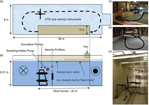
Wind in the tunnel was generated using a steel belt-drive ducted fan with a maximum rated flow of 430 m³ min⁻¹ that blew air through a flow straightener and along the water surface through the length of the wind tunnel. Wind produced in the wind tunnel was used to generate waves and water motion over a surface area of 40 m² that contained varying mixtures of water and ice, depending on the experiment. During the wind tunnel experiments, the rest of the tank surface did not experience any measurable breeze. Freezing of the water surface was produced by cooling the air inside the Test Basin over several days to produce a layer of columnar ice of 8.5 cm thickness and later of 18 cm thickness. The same approach was used to stimulate buoyant convection and gas exchange by convective turbulence. Ice thickness was measured using a Benthos PSA-916 sonar altimeter and by collecting 7.6 cm diameter ice cores. Further details on the bulk salinity, gas content and other ice properties are described by Lovely et al. (2015).

The design described above created a circulating ‘racetrack’ configuration that made it possible to introduce and quantify multiple processes that perturb the air–sea interface and lead to gas exchange. The design was modelled after annular wind wave tanks (Jahne et al., 1979; Mesarchaki et al., 2015); however, the constraints of an ice-strengthened containment vessel and environmental chamber, capable of achieving temperatures lower than −20 °C, did not permit the same level of symmetry as in an annular tank. The Test Basin and channel/tunnel configuration permitted gas exchange experiments to take place over the entire tank surface, when the ice was broken into floes. These are referred to as the ‘floe experiments’ (Experiments 1–12 in Table 1). Separately, the tank surface was frozen solid and a single opening or lead of varying length was created within the wind tunnel. These were the ‘lead experiments’ (Experiments 13–19 in Table 1). The lead experiments were used to estimate air–sea gas transfer as a result of wind, currents and wind + currents, and to measure small-scale processes that act on the water surface under reduced fetch conditions. Measurement of the wind speed inside the tunnel was carried out using Vaisala WS425 and WMT700 anemometers, both of which were suspended over the Test Basin from the roof of the wind tunnel. The height of the wind tunnel was 76 cm, and wind speed was measured vertically at two or more heights above the water surface by moving one anemometer vertically. The second anemometer remained stationary to measure wind speed always in the same location. The wind speed profile was used to estimate the drag coefficient (C _d), assuming a log linear relationship between wind speed and height above the water surface. Using C_d and the measured wind speed inside the wind tunnel, we subsequently calculated the 10 m wind speed (U₁₀), using the method described by Mesarchaki et al. (2015).

Table 1. Description of the physical properties and results from each of the gas exchange forcing experiments during GAPS

Experiment no.	Day of year	Forcing condition	Ice cover (1−f)	Open water (f)	Pump (Hz)	Air temperature (°C)	Water temperature (°C)	U10 (m/s)	C d wind	v (m s^−1)	z (m)	v ice (m s^−1)	k eff (m d^−1)	k (m d^−1)	Std. error in k
1	279	Convection	0.00	1.00	0	N/R	3.0	N/R	1.4E–03	0.00	0.00	0.00	0.57	0.57	0.34
2	295	Current	0.76	0.24	40	N/R	−1.5	N/R	1.4E–03	0.03	0.54	0.00	0.25	1.05	0.05
3	297	Current	0.39	0.61	40	−3.4	−1.4	N/R	1.0E–04	0.05	0.44	0.00	0.82	1.34	0.01
4	299	Current	0.39	0.61	60	−3.8	−1.4	3.46	1.4E–03	0.07	0.54	0.01	0.91	1.50	0.15
5	300	Current	0.39	0.61	20	−4.5	−1.4	2.69	2.0E–04	0.03	0.55	0.01	0.44	0.72	0.05
6	304	Current	0.21	0.79	60	−4.5	−1.4	2.35	3.0E–04	0.10	0.57	0.01	1.62	2.05	0.09
7	304	Current	0.21	0.79	40	−4.5	−1.4	1.29	2.8E–03	0.07	0.50	0.01	0.99	1.26	0.03
8	305	Current+convection	0.21	0.79	40	−10.0	−1.4	1.62	1.0E–04	0.06	0.55	0.01	1.55	1.96	0.02
9	305	Current	0.21	0.79	40	−2.8	−1.3	0.60	1.6E–01	0.06	0.49	0.01	1.17	1.49	0.07
10	306	Current	0.21	0.79	20	−2.9	−1.3	1.65	1.0E–04	0.03	0.53	0.01	0.36	0.46	0.10
11	309	Current	0.00	1.00	60	N/R	−1.2	1.29	1.0E–04	0.10	0.48	0.00	1.49	1.49	0.05
12	310	Current+convection	0.00	1.00	60	−18.0	−1.4	1.29	1.2E–03	0.09	0.47	0.00	3.44	3.44	0.41
13	313	Current	0.91	0.09	60	−2.8	−1.5	0.28	4.0E–04	0.24	0.51	0.00	0.26	2.85	0.20
14	316	Current	0.91	0.09	20	−6.1	−1.4	1.11	1.0E–04	0.07	0.51	0.00	0.13	1.44	0.17
15	320	Current+wind	0.91	0.09	5	−3.6	−1.4	6.65	1.0E–04	0.03	0.51	0.00	0.33	3.67	0.29
16	323	Wind	0.91	0.09	5	−3.4	−1.3	2.43	7.0E–04	0.02	0.51	0.00	0.00	0.02	0.34
17	334	Current+wind	0.96	0.04	60	−5.4	−1.5	3.91	6.0E–04	0.25	0.51	0.00	0.11	2.86	1.34
18	336	Wind	0.96	0.04	5	−3.4	−1.5	7.16	1.0E–03	0.02	0.51	0.00	0.03	0.65	0.48
19	339	Current+wind	0.96	0.04	40	−3.5	−1.5	5.67	3.0E–04	0.12	0.51	0.00	0.28	7.65	2.56

The forcing condition describes whether currents, wind and/or convection were in effect, which relates to the fan and water pump intensity (Hz). The wind speed profile was used to estimate the drag coefficient (C _d), assuming a log linear relationship between wind speed and height above the water surface. Using C _d and the measured wind speed inside the wind tunnel, we subsequently calculated the 10 m wind speed (U₁₀), using the method described by Mesarchaki et al. (2015). The term v _ice is the ice velocity, v is the water current speed; the difference between the two is the water–ice relative velocity (v _s) used in the text. The average values of k _eff, k and the standard deviation of k. C _d, drag coefficient.

Here, only a portion of the wind tunnel results – those results that could be gleaned from the tracer budgets – will be presented. The majority of the wind tunnel experiments, which involved measurement of the gradients in heat, moisture and pCO₂ above the water surface, will be described in a future publication.

2.2. Gas tracer methods for estimating k

To measure the rate of air–sea gas transfer, conservative gas tracers, SF₆, N₂O and ³He (for the lead experiments), were dissolved in the water of the Test Basin. This increased the aqueous concentration by 100–1000 times the ambient concentration for each gas so that evasion from the water was strongly favoured. The tracers were added to the tank after the ice cover had already formed so the initial gas concentration in the ice was effectively zero. Tracer was added between experiments on multiple occasions: on days 276, 293, 312 and 326. Both ice melt and ice formation can change the concentration of dissolved gases in the tank by dilution and by solute exclusion (Killawee et al., 1998); therefore, we sought to maintain a constant ice thickness. Tank salinity, visual inspection of the tank surface and ice cores were used to monitor the ice thickness and guard against freezing or melting; adjustments to the room temperature were made as needed.

Water samples for trace gas analysis were collected using a submersible pump that was positioned at the downstream end of the wind tunnel (see Fig. 1). It was determined that measuring the gas tracers in one location was adequate because the horizontal mixing time of the tank far exceeded the tank response time to gas exchange. The lateral mixing time in the Test Basin was determined by measuring a time series of CO₂ concentration during the addition of tracer to the Test Basin tank (Lovely et al., 2015). The rapid addition of 500 gallons of water supersaturated with CO₂ was mixed to produce a stable aqueous CO₂ concentration within 3 hours. In comparison, the values of water–air and water–ice flux lead to changes in the tank mass balance of ca. 5 % per 24 hours. By these measurements, the horizontal mixing time exceeded the gas exchange response time by a factor of 8.

N₂O and SF₆ were measured in 50 mL ground glass syringes via the headspace method (Ho et al., 2004). Approximately, 30 mL of ultra-high purity (UHP) nitrogen was added to each syringe before samples were equilibrated for 12 hours in a room temperature bath and shaken for 10 minutes to achieve solubility equilibrium (Wanninkhof et al., 1987). The gaseous samples were injected into an SRI-8610C gas chromatograph with an electron capture detector. Samples for ³He analysis were taken in copper tubes and analysed at the Lamont-Doherty Earth Observatory of Columbia University on a dedicated VG5400 mass-spectrometer (³He and ⁴He) and a Pfeiffer PrismaPlus quadrupole mass-spectrometer (Ne).

The time rate of change of these gas tracers provides a direct means to estimate k _eff. The mass balance of the inert gas tracers were used to infer gas flux from the water to the air and to the ice. Over short time intervals (i.e. days), the gas tracer mass balance in the tank was determined by3

is the change in tracer mass in the Test Basin through time, F _ice is the flux of tracer from the water to the ice and F _air is the flux of tracer from the water to the air. F _air and F _ice depend on the air–water and air–ice transfer velocities (k and k _ice), and on the concentration gradients between the water, ice and air. After correcting for tracer loss to the ice [using eq. (3)], the values of k _eff were determined, and the values of k were solved using eq. (2) together with k _eff and f as the inputs. Because a correction for F _ice was previously made to the tracer budget, k _ice was set equal to zero for the determination of k. Additionally, a correction for brine drainage and ice melt was made to the tracer mass balance presented here and in Lovely et al. (2015). Collectively, the corrections account for less than 5 % of the observed change in the tracer mass balance within the Test Basin. Table 1 contains the values of k and k _eff, as well as f, but we exclusively use k in the figures, results and discussion because the areal dependence is removed. All the values of k, k _eff and k _ice have been normalised to a Schmidt number of 660 for purposes of comparison with other studies. Additional results of the experiment, including estimates of gas diffusion through the ice, and ice–water partitioning of He, Ne, SF₆ and N₂O are presented in Lovely et al. (2015). A time-lapse video of the evolution of the ice on the Test Basin can be viewed at https://youtube/-IgVl0qYKaY.

Altogether, the results from the lead and floe experiments were used to quantify the air–water gas transfer velocity at six different percent ice covers: 96, 91, 76, 39, 21 and 0 %. The effect of convection on gas exchange was estimated at 21 and 0 % ice cover. Gas transfer from wind and wind + currents was measured at 96 and 91 % ice cover. Estimates of k _eff were determined independently for the mass balance of each tracer: SF₆, N₂O and ³He. The uncertainty on each estimate of k _eff was computed using the standard deviation of these independent estimates.

3. Ice, currents and shear in the IOBL

3.1. Ice properties and ice velocity during GAPS

The percent ice cover during experiments 1 through 12 (76±1.6 %, 39±2.2 % and 21±6 %) was estimated using image analysis of the ice, which was broken into small floes (1×0.5 m). At 91 and 96 % ice cover, during lead experiments in the wind tunnel, we were able to directly measure the length, width and geometry of the rectangular opening in the ice.

The velocity of individual ice floes circulating through the Test Basin was estimated by observing the strength of acoustic reflection (db) as measured by the Nortek Acoustic Doppler velocity Profilers (ADPs). More details about the ADPs can be found in Section 3.2. As the ice floes pass above the submerged ADP, the strong acoustic reflection off the ice surface can be used to determine the travel time for the floe to pass (Supplementary Fig. 1). Using the average sea ice floe length (0.9 m), we determined the average ice velocity by dividing the floe length by the average travel time over the ADP during each experiment. The average ice velocity for each of the gas exchange experiments can be found in Table 1. Ice velocity was zero during lead mode at 91 and 96 % ice cover, because a single sheet of ice covered the Test Basin. When the ice cover was 75 % or greater, there was essentially no ice movement, the ice floes became jammed and did not circulate freely. At 39 % ice cover, ice velocity ranged from 0.4 to 0.7 cm s⁻¹. At 21 % ice cover, the ice circulated more freely, and the ice velocity was consistently 0.7 cm s⁻¹.

3.2. Current shear stress in the IOBL

Current speeds in the Test Basin were measured at two locations in the tank using the ADPs; one in the channel just upstream from the pumps and the second in the main part of the Test Basin where the return flow occurred (see Fig. 1 for locations). Velocity profiles from multiple experiments are featured in Fig. 2. Comparing velocity profiles between instances when the tank was ice-free and when the tank was ice-covered it is apparent how the presence of ice cover exerts a drag on the water surface. Figure 2 also contrasts velocity profiles in the channel when the fan was blowing wind over the water surface, versus when the fan was off, but the pumps were circulating water.

Fig. 2 Profiles of water velocity measured by acoustic Doppler profiler in the ‘channel’ beneath the wind tunnel and in the ‘tank’ outside the wind tunnel. The panels labelled ‘Ice-free’ show velocity during a coincident 12-hour period in the tank and channel with no ice cover. The panels labelled ‘Ice cover’ and ‘Open lead’ (black profiles) show velocity profiles during a coincident 22-hour period. The channel velocity was measured beneath a ‘lead’ opening in the ice, so it was never directly ice covered. The red profile in panel 4 reflects wind forcing with almost no water pump forcing.

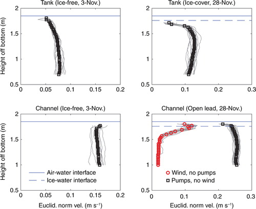
There is an inherent trade-off in the ADP between the depth field over which velocity is measured and the magnitude of the velocity that can be resolved (Rusello, 2009). To ensure that we could capture the maximum expected velocity, it was not possible to place the ADP on the bottom and measure the full water column velocity profiles. The ADPs in the channel and tank were 1.04 and 1.34 m, respectively, below the water surface. Consequently, the vertically averaged velocity does not capture the deepest portion of the velocity profile. The tank bottom (in addition to the ice) is expected to exert a drag on the water surface; however, the velocity profiles do not show strong evidence of bottom drag or curvature in the velocity profiles at depths of 0.75 to 1 m above the bottom.

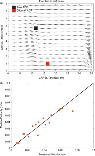
The ‘racetrack’ circulation in a rectangular tank lacks the even curvature of an annular tank; consequently, the flow velocity and surface stress are not the same everywhere, leading to heterogeneities in the flow field. As we are generating estimates of air–sea gas exchange for the entire Test Basin, it was necessary to capture the structure of the velocity field throughout the tank. This was accomplished with a 2-D model of the shallow water flow equations with variable density (Loose et al., 2005). The model produces a horizontal flow field that represents the vertically averaged velocity at each position in the tank (Fig. 3, left panel). To test the accuracy of the model, we forced it with the average velocity measured in the channel and compared the resulting model velocity in the tank where the second ADP was located (Fig. 3, right panel). We compared the model velocity and daily measurement of average velocity for each of the 20 d of the floe experiment and found good agreement between the model and the ADP in the tank; the average absolute difference between modelled and measured velocity was 14 %. The model further predicts that when the average velocity in the channel exceeded 5 cm s⁻¹, a recirculation eddy was produced along the northwest side of the channel wall (Fig. 3). This is consistent with our visual observations of the circulation in the Test Basin.

Fig. 3 (Left) Flow field as determined by a finite volume solution to the Boussinesq equations with variable density (Loose et al., 2005). The mean shear velocity (v _s) produced in the channel is 0.047 m s⁻¹ in the simulation that is depicted. Right panel, a comparison between measured v _s by the Tank ADP and the modelled velocity at that location. Forcing for each simulation was produced using the values of v _s that were measured at the Channel ADP location as input, reflecting the action of the circulation pumps.

The model-weighted average water velocity (v) and ice velocity (v _ice) for each lead and flow experiment are listed in Table 1. The water velocity ranged from 0 to 0.25 m s⁻¹, and ice velocity was always less than 0.01 m s⁻¹ (see Section 3). We refer to the difference between the ice velocity and the water velocity as v _s, or shear velocity to indicate that this is the relative velocity producing shear at the air–water and ice–water interface. The values of v _s also ranged from 0 to 0.25 m s⁻¹. It is also worth noting that v _ice was zero during the lead experiments, because the ice was wedged against the walls of the tank.

To put the laboratory-based values of v _s into context, we can compare them with the daily-averaged values of the velocity difference between sea ice and seawater at 10 m depth for velocities measured in the Arctic Ocean from an Ice-Tethered Profiler (ITP). ITP-35 (http://www.whoi.edu/itp) was deployed on October 2009 and recorded data until March 2010. During this period of relatively high ice cover (Cole et al., 2014), v _s ranged between 0.05 and 0.3 m s⁻¹ with a mean value of 0.09 m s⁻¹. These velocity measurements from the Arctic Ocean indicate that the values of v _s produced during the GAPS experiments are representative of the range observed in the Arctic sea ice zone.

3.3. Gas exchange driven by ice–water current shear

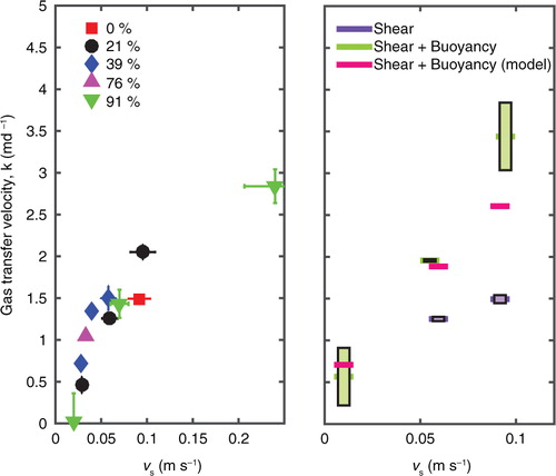
If we select the experiments where v _s was the only significant source of boundary layer turbulence near the ice–water interface (i.e. no convection and minimal wind), a clear increasing trend emerges between v _s and k (Fig. 4, left panel). The values have been symbol coded to distinguish the different percent ice covers during each experiment. It is apparent, from this coding that there is no discernible relationship between k and the amount of ice cover. This is as expected, based on eq. (2), we know that k is an intensive property that reflects only the kinetics regulating gas transport, and unlike k _eff, does not contain an explicit dependence on the area of open water. During these experiments, a maximum of v _s=0.25 m s⁻¹ produced a k of 2.8 m d⁻¹. In comparison, the quadratic wind speed relationship for the open ocean (Wanninkhof, 2014) produces approximately the same value of k for a wind speed of 7 m s⁻¹. It is important to note that significant gas exchange occurred during Experiment 11 (Table 1), when no ice cover was present (red square in Fig. 4). In this circumstance a boundary current shear can still exist at the air–water interface (Edson et al., 2007). The resulting gas exchange cannot be interpreted as driven by ice–water current shear, but the results show that the scaling between k and shear velocity remains consistent at all fractions of ice cover, including zero.

Fig. 4 (Left) Relationship between the water–ice relative velocity (v _s) and k for all of the experiments, where v _s was the only significant source of turbulence at the air–sea interface. (Right) The gas transfer velocity produced shear + convection (green lines), as compared with the model for gas transfer as a function of TKE dissipation (Zappa et al. 2007) (pink bars). For reference, the k by shear alone (purple bars) has been included at v _s=0.06 and 0.09 m s⁻¹ to illustrate the enhancement that results from convection. The shaded black boxes represent the standard error in the estimates of k.

4. Gas exchange driven by convection in the IOBL

During the three experiments, we measured the air–sea gas transfer velocity while attempting to produce convection in the Test Basin by lowering the air temperature in the room. The tank surface was monitored closely for evidence of skim ice, because ice formation will alter the surface area for gas exchange and change the gas concentration as described in Section 2.2. The first experiment involved only convection, that is, the pumps were turned off to eliminate shear-driven mixing. This was possible because the water temperature was 2.6 °C, that is, the water was far from the freezing point, so freezing of the water surface was precluded by continual renewal of warmer water from below. This experiment took place before the first layer of ice was formed on the tank surface. The subsequent convection events took place at 21 and 0 % ice cover, while the water was close to the freezing point. To avoid skim ice formation at the edges and stagnation points, the pumps were used to circulate water in the tank.

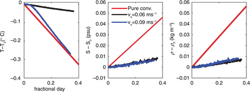
Convection can be inferred from the loss of buoyancy, which in turn can be observed from the decreases in temperature and increases in salinity during each experiment (Fig. 5). By comparing measured values of k from current shear alone with the values of k produced by current shear + convection, we can infer the increase in k caused by convection. Comparing Experiment 7 with Experiment 8, we observed an increase of 56 % from k=1.26 to k=1.96 m d⁻¹, as a result of convection. Comparing Experiment 11 with Experiment 12, we observed a 131 % increase in k beyond that produced by shear alone, from k=1.49 to k = 3.44 m d⁻¹ (Fig. 4, right panel).

Fig. 5 (Left, middle and right) Temperature, salinity and the resulting density changes during the three convection events where buoyancy losses from the Test Basin were used to induce air–sea gas exchange. The initial T, S conditions for the three events were as follows: Experiment 1, Pure convection: (2.7, 26.4), Experiment 8, v _s=0.06: (−1.1, 26.9), Experiment 12, v _s=0.09: (−1.44, 26.9).

We can further compare the laboratory measurements of k with predictions of k, produced by shear and convection using Monin–Obukhov similarity theory (MOST) and the empirical MOST relationships developed by Lombardo and Gregg (1989). The empirical MOST relationships from Lombardo and Gregg (1989) were developed from observations of night-time convection in the equatorial ocean, but the primary diagnostic variable is the intensity of the boundary layer current shear. Based on the principles of similarity theory, we expect these relationships to be applicable to the ice–ocean boundary layer in the absence of active freezing, as was the case in these experiments.

Using MOST, the effect of shear and convection on water surface turbulence can both be expressed in terms of the Turbulent Kinetic Energy Dissipation (ɛ), which has units of power per unit mass (Watts per kilogram, or alternately m² s⁻³). To estimate the total ɛ in the presence of convection and currents, we first computed the shear-driven dissipation (ɛ_s) using the values of v _s and z – the mean measurement depth – from Table 1 by

κ is the Von Karmann constant, and z ₀ is the roughness length (Lombardo and Gregg, 1989). The values of ɛ_s indicate that the second two convection experiments (Experiments 8 and 12, Table 1) fall into a regime dominated by shear. Thus, we used the following similarity scaling,5

The term J _b refers to buoyancy loss from convection, which was determined from the observations of temperature and salinity change in the Test Basin (Fig. 5) and the seawater equation of state. Finally, k was calculated from ɛ using (Lamont and Scott, 1970; Zappa et al., 2007),6 where ν is the kinematic viscosity of water, and Sc is the Schmidt number. The above equations describe bulk values of turbulent dissipation in the ice–water boundary layer, whereas sometimes varies vertically up to the ocean surface (Lombardo and Gregg, 1989).

In the convection-only event (Experiment 1), eq. (6) predicts a value of k=0.71±0.05 m d⁻¹. In comparison, the N₂O, SF₆ tracer budgets yielded an estimate of k=0.56±0.35 m d⁻¹ (a 21 % difference). The N₂O, SF₆ tracer budget estimates of k during convection + shear (Experiment 8 and 12, Table 1) were 1.96±0.02 and 3.4±0.4 m d⁻¹. Collectively, these three measured estimates of k fall within a range of 6–27 % of eq. (6) predictions (pink bars in Fig. 4, right panel), indicating agreement between the predicted and measured estimates of k from convection and current shear. These observations of enhanced k from convection are consistent with the observations of gas transfer driven by night-time convection in the equatorial Pacific by McGillis et al. (2004). The diel heating and cooling of the equatorial surface ocean lead to convective velocities that would exceed the shear-driven velocity at night. The measurements of enhanced k from night-time convection occurred at wind speeds less than 6 m s⁻¹ (McGillis et al., 2004). This study estimated that the net annual contribution of night-time convection to the CO₂ flux was on the order of 40 % of the total annual flux.

5. Gas exchange by wind + currents

The experiments involving wind + currents (Experiments 15–19) produced the widest range of scatter in k that we observed; these are the red circles in Fig. 6. The maximum was 7.65 m d⁻¹ and the minimum was 0.03 m d⁻¹. Using the tracer mass balance for the entire tank to estimate gas transfer driven by wind was the most challenging aspect of these experiments, because the air–sea gas fluxes are restricted to a small area of open water inside the wind tunnel (9 and 4 % of the tank surface). At the same time, stronger winds and weaker currents in the tank tended to produce freezing at the ice edge, which complicated the tracer budget and reduced the surface area for gas exchange. Consequently, gas-exchange forcing by the wind is the least well constrained of the forcing in the GAPS experiments.

Fig. 6 The gas transfer velocity, k, compared with the average 10 m wind speed in the wind tunnel during the given experiment. The ‘square’ symbols denote estimates during the floe experiments, where open water existed outside the wind tunnel.

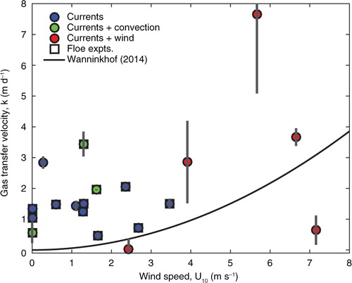
Despite these shortcomings, we have opted to include these data in the interpretation, because they can provide some preliminary insights and because there are no other laboratory measurements of this type for ice-covered water. Three of the five wind + currents experiments (Experiments 15, 17 and 19) produced values of k that exceed the wind speed scaling of Wanninkhof (2014) (Fig. 6). Not surprisingly, the measurements of k from current shear and convection also exceeded the wind speed scaling.

In contrast, experiments 16 and 18 yielded values of k that were significantly smaller than what would be predicted from the wind speed parameterisation of Wanninkhof (2014) (Fig. 6). These two experiments were distinct from the others in that we attempted to measure gas exchange forced by wind alone, without currents. However, it proved necessary to retain a minimal circulation of the water to avoid freezing. The mean value of v _s was 0.02 m s⁻¹, measured directly beneath the lead. During these experiments, k was 0.02±0.34 m d⁻¹ at U₁₀=2.4 m s⁻¹ and 0.65±0.48 m d⁻¹ at U₁₀=7.1 m s⁻¹ wind. At this wind speed, the quadratic wind speed parameterisation (Wanninkhof, 2014) predicts 0.3 and 3.0 m d⁻¹, respectively. One explanation for these unexpectedly low estimates is inadequate surface renewal of water directly beneath the lead opening in the ice. Because the circulation in the Test Basin was very low, the water trapped in the lead opening may have been stagnated and depleted of gas. Without replenishment, the gas partial pressure differential would become diminished, leading to a decreased gas flux and corresponding decrease in the estimate of k. Under some circumstances, the same phenomenon might occur in the real ice–ocean boundary layer; however, Ekman turning is a persistent feature of the IOBL, leading to continual relative motion between the ice and the water beneath it (McPhee, 1992). Additionally, lead openings produce their own local circulation (Morison et al., 1992), which would also lead to surface gas renewal. The low surface renewal might explain the low values of k during experiments 16 and 18; however, the current speed was nearly as low during experiment 15 when the tracers predicted a much greater value of k. Aside from the uncertainty in the tracer mass balance when the open water area is low and fluxes are small, we have no adequate explanation for these apparently contradictory results. Consequently, the scaling of air–sea gas transfer when fetch is reduced by high ice cover persists as an unanswered question. During all other experiments, the pumps were operated to produce current shear beneath the ice, and Lovely et al. (2015) have shown that the mixing time is much faster (ca. 20 minutes) than the gas transfer response time (ca. 1–3 d) when the water is being circulated.

6. Scaling between k and ɛ

Because the quadratic wind speed parameterisation does not reflect sources of turbulence, such as those that occur in the IOBL, it is helpful to examine the gas transfer velocity using a forcing metric that is common across each process; ɛ is presently the best available metric. Here, we have estimated ɛ using the parameter model described by Loose et al. (2014). The parameter model uses boundary layer scaling for the ice–ocean boundary layer (McPhee, 2008) and MOST (Lombardo and Gregg, 1989) to estimate ɛ from buoyancy changes and current shear, as described in Section 4. At a minimum, the parameter model requires the following inputs: v _s, f, water temperature and air temperature. It should be noted that this parameter model provides bulk values of ɛ in the IOBL, while it is known that ɛ can vary vertically up to the air–sea interface (Lombardo and Gregg, 1989).

The values of v _s were computed as described in Section 3.2 using the velocity profiles collected by the Nortek ADPs (as in Fig. 2) and model-derived flow field to produce a tank-wide average of v _s. The values of f were calculated from the fraction of ice cover described in Section 3.1, the water temperature was measured by Conductivity-Temperature-Depth sensor (CTD) in the tank (Lovely et al., 2015) and the air temperature was measured in the wind tunnel. Finally, the parameterised estimates of k are computed using eq. (6) and related to the tracer mass balance estimates.

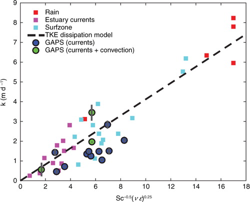
The comparison of Turbulent kinetic energy (TKE) dissipation scaling with tracer-based estimates of k is found in Fig. 7. As an aggregate, the measurements of k and estimates of ɛ during the GAPS experiment cluster around the slope of 0.419 that was proposed by Zappa et al. (2007), yet many of the ‘current only’ experiments fall below the 0.419 slope (Fig. 7). A linear fit to the ‘current only’ experiments result in a slope of 0.27, indicating a smaller proportionality between ɛ and k. However, it is not possible to conclusively substantiate a different relationship between ɛ and k, because our estimates of ɛ are based upon bulk ice–ocean boundary layer parameters instead of more direct estimates of ɛ near the water surface. While it is not possible to definitively evaluate the proportionality between k and ɛ, it is interesting to compare the dynamic range in k produced by shear and convection in the IOBL, in comparison to estimates in other environments. The comparison indicates that gas exchange in the IOBL shows similar energetics as weak surf zone and estuarine turbulence, but is less vigorous than gas exchange driven by rain.

Fig. 7 Scaling between gas transfer velocity (k) and TKE dissipation (ɛ), from Lamont and Scott (1970). The coloured squares originate from Zappa et al. (2007), indicating estimates of gas transfer driven by rain, estuarine tidal processes and surf zone turbulence.

The estimates of k during wind + current forcing were not included in Fig. 7, because we lack the information from literature or observations to convert measurements of the wind speed to estimates of ɛ at the ocean surface, which is a significant gap in our understanding of air–sea gas exchange in the IOBL. In another study of turbulence in an estuary (Zappa et al., 2007), the contribution of currents to the total turbulence budget became minimal as the wind speed exceeded 5 m s⁻¹. In these experiments, we found some evidence for enhanced gas exchange, at similar wind speeds, when wind and currents are both present. This mechanism of enhancement may be unique to the sea ice zone, where currents beneath the ice act to replenish the openings with gas-rich water that helps to maintain the air–sea concentration gradient and avoid having degassed water stagnate within the openings. Divergent flow between ice and water due to Ekman and buoyancy forcing is characteristic of the sea ice zone (Geiger and Drinkwater, 2005; Cole et al., 2014).

7. Summary and conclusions

During design of the GAPS experiment, considerable effort was made to hew close to the proven experimental techniques used in earlier gas exchange experiments [e.g. Jahne et al., (1979)] while coping with the limitations imposed by growing and maintaining ice cover in a laboratory setting. These trade-offs resulted in several acknowledged shortcomings, most importantly that the flow field is not uniform throughout the tank as it would be in an annular wind-wave tank, and it was not possible to measure water velocity everywhere in the tank. Despite these shortcomings, the rectangular geometry of the tank and the steady-state circulation leads to a stationary flow that is straight forward to model using computational fluid dynamics. This is demonstrated by the agreement between modelled velocity and the velocity measured by the tank ADP (Fig. 3, right panel).

Another shortcoming of such a tank experiment is the drag produced by the bottom and sides of the tank, which would not be present in the real IOBL. While the bottom boundary may have impacted the overall drag on the water column, there is not much evidence of curvature in the velocity profiles near 1 m in Fig. 2, as might be expected if a bottom boundary layer was strongly impacting the velocity profile. In contrast, both ice and wind had a demonstrable impact on the shape of the velocity profiles. It is also worth pointing out that enhancement of gas exchange is thought to occur by eddies that impinge on the viscous mass boundary layer at the air–sea interface. The viscous boundary layer is ca. 100 µm in thickness and directly adjacent to the air–sea interface, implying that eddies generated in the far field (sides and bottom) have much less impact than processes acting at the air–sea interface (i.e. sea ice drag, convection, and wind). The flow characteristics, including flow rate, position and location of the submersible pumps were designed to capture the range of current speeds that have been measured in the IOBL, and this can be observed by comparing with ITP-V data from the Arctic presented by Cole et al. (2014). The ice is stationary or drifting does not matter, as the important factor for generating shear is the relative difference between ice and water velocity.

Keeping in mind the inherent shortcomings of such a laboratory experiment, there are significant advantages to such studies, as they permit us to isolate, combine and control processes in order to compare and contrast the impact of each process.

The GAPS experiments have demonstrated that the rate of air–water gas transfer positively co-varies with current shear and buoyancy losses in the IOBL. These processes produced first-order gas transfer velocities in a laboratory setting and we can infer that they significantly altered boundary layer turbulence and the buoyancy budget within Test Basin. The impact of ice drift and buoyancy forcing may be even more important in the IOBL where fetch is reduced, and ice cover all but eliminates the impact that ocean swell, breaking waves and air-bubble injection have on the transfer velocity.

Although these experiments demonstrate the significant influence of current shear and buoyancy on the rate of air–sea gas transfer, the experiments yielded less conclusive results regarding the effect of wind and wind + current shear in the IOBL. When wind and currents acted in combination to produce aqueous turbulence, the resulting estimates of k were enhanced if compared with the quadratic wind speed parameterisation that is most frequently used to estimate k. However, shortcomings in the experimental configuration precluded making reliable measurements from k alone in reduced fetch conditions. We still know very little about how turbulence from wind is modulated by the presence of sea ice. High wind speeds are known to transfer momentum through the ice to the water column; however, it is unclear whether gas transfer velocity experiences a rapid non-linear increase as wind builds above 10 m s⁻¹. This study demonstrates that wind speed alone is not sufficient to predict the rate of air–sea gas exchange in the sea ice zone.

8. Acknowledgements

The authors would like to thank Leonard Zabilansky, Thomas Tantillo, Gordon Gooch and the rest of the engineering staff at CRREL. Brent Else and one anonymous reviewer provided feedback that was exceedingly valuable in revising the manuscript. Funding support for GAPS and for B. Loose, P. Schlosser, C.J. Zappa, W.R. McGillis and D. Perovich was provided by NSF ANT 09-44643. Given the nature of this data as laboratory based, we have opted not to submit to an oceanographic repository but all the data have been archived and are available by contacting Brice Loose ([email protected]).

Notes

To access the supplementary material to this article, please see Supplementary files under ‘Article Tools’.

References

- Butterworth B. J., Miller S. D. Air-sea exchange of carbon dioxide in the Southern Ocean and Antarctic marginal ice zone. Geophys. Res. Lett. 2016; 43(13): 7223–7230. DOI: http://dx.doi.org/10.1002/2016GL069581.
- Cole S. T., Timmermans M.-L., Toole J. M., Krishfield R. A., Thwaites F. T. Ekman veering, internal waves, and turbulence observed under Arctic Sea ice. J. Phys. Oceanogr. 2014; 44(5): 1306–1328. DOI: http://dx.doi.org/10.1175/JPO-D-12-0191.1.
- de Lavergne C. , Palter J. B. , Galbraith E. D. , Bernardello R. , Marinov I . Cessation of deep convection in the open Southern Ocean under anthropogenic climate change. Nat. Clim. Change. 2014; 4(4): 278–282.
- Delille B., Vancoppenolle M., Geilfus N.-X., Tilbrook T., Lannuzel D., co-authors. Southern Ocean CO2 sink: the contribution of the sea ice. J. Geophys. Res. Oceans. 2014; 119(9): 6340–6355. DOI: http://dx.doi.org/10.1002/2014JC009941.
- Edson J., Crawford T., Crescenti J., Farrar T., Frew N., co-authors. The coupled boundary layers and air–sea transfer experiment in low winds. Bull. Am. Meteorol. Soc. 2007; 88(3): 341–356. DOI: http://dx.doi.org/10.1175/BAMS-88-3-341.
- Else B., Papakyriakou T., Galley R. J., Drennan W. M., Miller L. A., co-authors. Eddy covariance measurements of wintertime CO2 fluxes in an arctic polynya: evidence for enhanced gas transfer during ice formation. J. Geophys. Res. 2011; 116: C00G03. DOI: http://dx.doi.org/10.1029/2010JC006760.
- Fanning K. A. , Torres L. M . 222Rn and 226Ra: indicators of sea-ice effects on air-sea gas exchange. Polar. Res. 1991; 10: 51–58.
- Geiger C. A., Drinkwater M. R. Coincident buoy – and SAR-derived surface fluxes in the western Weddell Sea during Ice Station Weddell 1992. J. Geophys. Res. 2005; 110: 1–16. DOI: http://dx.doi.org/10.1029/2003JC002112.
- Ho D. T., Zappa C. J., McGillis W. R., Bliven L. F., Ward B., co-authors. Influence of rain on air-sea gas exchange: lessons from a model ocean. J. Geophys. Res. Oceans. 2004; 109: 1–15. DOI: http://dx.doi.org/10.1029/2003JC001806.
- Jahne B., Münnich K. O., Siegenthaler U. Measurements of gas exchange and momentum transfer in a circular wind-water tunnel. Tellus. 1979; 31(4): 321–329. DOI: http://dx.doi.org/10.1111/j.2153-3490.1979.tb00911.x.
- Killawee J. A. , Fairchild I. J. , Tison J.-L. , Janssens L. , Lorrain R . Segregation of solutes and gases in experimental freezing of dilute solutions: implications for natural glacial systems. Geochim. Cosmochim. Acta. 1998; 62: 3637–3655.
- Kitidis V., Upstill-Goddard R. C., Anderson L. G. Methane and nitrous oxide in surface water along the North-West Passage, Arctic Ocean. Mar. Chem. 2010; 121: 80–86. DOI: http://dx.doi.org/10.1016/j.marchem.2010.03.006.
- Lamont J. C. , Scott D. S . An eddy cell model of mass transfer into the surface of a turbulent liquid. AIChE J. 1970; 16: 512–519.
- Lombardo C. P. , Gregg M. C . Similarity scaling of viscous and thermal dissipation in a convecting surface boundary layer. J. Geophys. Res. 1989; 94: 6273–6284.
- Loose B., McGillis W. R., Perovich D., Zappa C. J., Schlosser P. A parameter model of gas exchange for the seasonal sea ice zone. Ocean. Sci. 2014; 10: 17–28. DOI: http://dx.doi.org/10.5194/os-10-17-2014.
- Loose B. , Nino Y. , Escauriaza-Mesa C . Finite volume modeling of variable density shallow-water flow equations for a well-mixed estuary: application to the Rio Maipo estuary in central Chile. J. Hydraul. Res. 2005; 43(4): 339–350.
- Loose B., Schlosser P. Sea ice and its effect on CO2 flux between the atmosphere and the Southern Ocean interior. J. Geophys. Res. Oceans. 2011; 116 DOI: http://dx.doi.org/10.1029/2010JC006509.
- Lovely A., Loose B., Schlosser P., McGillis W., Zappa C., co-authors. The gas transfer through Polar Sea ice experiment: insights into the rates and pathways that determine geochemical fluxes. J. Geophys. Res. Oceans. 2015; 120(12): 8177–8194. DOI: http://dx.doi.org/10.1002/2014JC010607.
- Mathis J. T., Cross J. N., Monacci N., Feely R. A., Stabeno P. Evidence of prolonged aragonite undersaturations in the bottom waters of the southern Bering Sea shelf from autonomous sensors. Underst. Ecosyst. Process. East. Bering. Sea. III. 2014; 109: 125–133. DOI: http://dx.doi.org/10.1016/j.dsr2.2013.07.019.
- McGillis W. R., Edson J. B., Zappa C. J., Ware J. D., McKenna S. P., co-authors. Air-sea CO2 exchange in the equatorial Pacific. J. Geophys. Res. 2004; 109: C08S02. DOI: http://dx.doi.org/10.1029/2003JC002256.
- McPhee M. G . Turbulent heat flux in the upper ocean under sea ice. J. Geophys. Res. 1992; 97: 5365–5379.
- McPhee M. G . Air-Ice-Ocean Interaction: Turbulent Ocean Boundary Layer Exchange. 2008; Springer, New York.
- Mesarchaki E., Kräuter C., Krall K. E., Bopp M., Helleis F., co-authors. Measuring air–sea gas-exchange velocities in a large-scale annular wind–wave tank. Ocean. Sci. 2015; 11(1): 121–138. DOI: http://dx.doi.org/10.5194/os-11-121-2015.
- Miller L., Papakyriakou T., Collins R. E., Deming J. W., Ehn J. K., co-authors. Carbon dynamics in sea ice: a winter flux time series. J. Geophys. Res. 2011; 116 DOI: http://dx.doi.org/10.1029/2009JC006058.
- Morison J. H. , McPhee M. , Curtin T. B. , Paulson T. B . The oceanography of winter leads. J. Geophys. Res. 1992; 97: 11199–11218.
- Rusello P . A Practical Primer for Pulse Coherent Instruments. 2009; Technical Note, Nortek AS, Bergen, Norway.
- Rutgers Van Der Loeff M., Cassar N., Nicolaus M., Rabe B., Stimac I. The influence of sea ice cover on air-sea gas exchange estimated with radon-222 profiles. J. Geophys. Res. Oceans. 2014; 119: 2735–2751. DOI: http://dx.doi.org/10.1002/2013JC009321.
- Shakhova N., Semiletov I., Leifer I., Salyuk A., Rekant P., co-authors. Geochemical and geophysical evidence of methane release over the East Siberian Arctic Shelf. J. Geophys. Res. Oceans. 2010; 115: C08007. DOI: http://dx.doi.org/10.1029/2009jc005602.
- Wanninkhof R. Relationship between wind speed and gas exchange over the ocean revisited. Limnol. Oceanogr. Methods. 2014; 12(6): 351–362. DOI: http://dx.doi.org/10.4319/lom.2014.12.351.
- Wanninkhof R., Ledwell J. R., Broecker W. S., Hamilton M. Gas exchange on Mono Lake and Crowley Lake, California. J. Geophys. Res. Oceans. 1987; 92(C13): 14567–14580. DOI: http://dx.doi.org/10.1029/JC092iC13p14567.
- Zappa C. J. , Raymond P. , Terray E. , McGillis W. R . Variation in surface turbulence and the gas transfer velocity over a tidal cycle in a micro-tidal estuary. Estuaries. 2003; 26: 1401–1415.
- Zappa C. J., McGillis W. R., Raymond P. A., Edson J. B., Hintsa E. J., co-authors. Environmental turbulent mixing controls on air–water gas exchange in marine and aquatic systems. Geophys. Res. Lett. 2007; 34 DOI: http://dx.doi.org/10.1029/2006GL028790.