The Effectiveness of Rotating Tank Experiments in Teaching Undergraduate Courses in Atmospheres, Oceans, and Climate Sciences

ABSTRACT

While it is commonly recognized that laboratory experiments and demonstrations have made a considerable contribution to our understanding of fluid dynamics, few U.S. universities that offer courses in meteorology and/or oceanography provide opportunities for students to observe fluid experiments in the classroom. This article explores the evaluation results of a three-year, NSF-funded project in partnership with the Massachusetts Institute of Technology (MIT) and five universities nationally, to provide laboratory demonstrations, equipment, and curriculum materials for use in the teaching of atmospheres, oceans, and climate. The aim of the project was to offer instructors a repertoire of rotating tank experiments and a curriculum in fluid dynamics to better assist students in learning how to move between phenomena in the real world and basic principles of rotating fluid dynamics, which play a central role in determining the climate of the planet. The evaluation highlights the overwhelmingly positive responses from instructors and students who used the experiments, citing that the Weather in a Tank curriculum offered a less passive and more engaged and interactive teaching and learning environment. Results of three years of pre- and posttesting on measures of content related to atmospheres, oceans, and climate sciences with over 900 students in treatment and comparison conditions, revealed that the treatment groups consistently made greater gains at the posttest than the comparison groups, especially those students in introductory level courses and lab courses.

Key words::

• education testing and evaluation
• education science experiments
• education undergraduate
• atmospheric and oceanic sciences
• teaching and curriculum
• climate
• fluids
• rotating fluids
• geophysical fluid dynamics

Acknowledgments

We would like to thank the students and professors of the collaborating universities for their interest in and support of the Weather in a Tank project, and the National Science Foundation (NSF), whose support made this project possible.

FIGURE 1: (Left) A laboratory analogue of weather systems in which an ice can placed in the middle of a rotating tank of water induces a radial temperature gradient. The presence of eddies in the tank, analogous to the atmospheric weather systems shown on the right, can be seen through the swirling dye patterns. (Right) A view of temperature variations at a height of 2 km showing swirling regions of warm (red) and cold (blue) air associated with synoptic-scale weather systems. The North Pole is indicated by the white dot at the upper left of the figure. See http://paoc.mit.edu/labguide. See online article to view color version of figure.

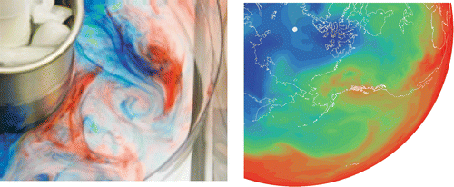
FIGURE 2: (Top left) The plastic bucket on the dial of a rotating turntable in which a laboratory vortex is formed. (Top right) The trajectory of a paper dot floating on the free surface of the vortex formed from water spiraling inward toward the drain hole. (Bottom left) Spiral cloud formations associated with Hurricane Bertha on September 7, 2008. (Bottom right) Streamlines of surface flow around the eye of Hurricane Bertha on September 7, as revealed by QuikScat wind data.

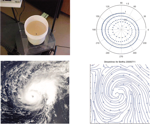
FIGURE 3: Significance of the Rossby number as it relates to balance of forces, F. Planetary-scale flows on the earth have small Rossby numbers, indicating a balance between pressure gradient and Coriolis forces. Smaller-scale weather systems and fronts have Rossby numbers of order unity, indicating that centrifugal forces also play a role. In hurricanes and tornadoes indicated on the right, Rossby numbers become very large (exceeding 10) and Coriolis plays a negligible role in the force balance. The balanced vortex laboratory experiment illustrates the balance of forces across this whole range of Rossby number.

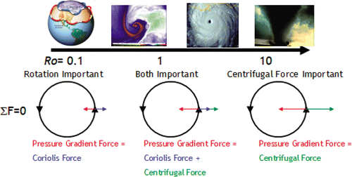
FIGURE 4: (Left) Rossby number (Ro) plotted as a function of the particle's radius (in cm). (Right) The Rossby number plotted as a function of radius (km) for Hurricane Bertha, using near-surface winds from QuikScat data.

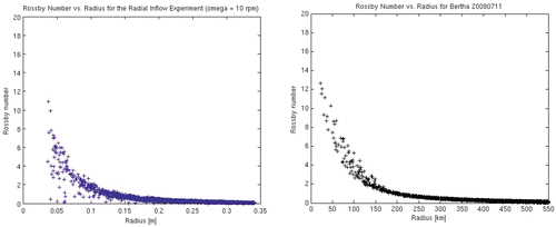
FIGURE 5: Collaborating universities and professors.

FIGURE 6: Two sample questions from the pre- and posttest. The full test is a 27-item, multiple-choice test covering general content related to atmospheres, oceans, and climate sciences, such as the importance of the earth's rotation on atmospheric circulation, the underlying cause of seasons, and reasons for typical wind speeds. This test was designed specifically for the Weather in a Tank project, but with an eye for wider, more general use. It is available on request from Lodovica Illari.

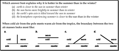
FIGURE 7: Frequency of experiment use by instructors, spring 2007–Spring 2009. “A” indicates experiments used in atmosphere classes; “O” represents classes in oceanography, and “AO” indicates atmosphere and/or oceanography courses. A full description of these and other experiments can be found on the project website.

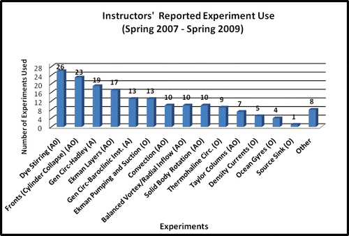
FIGURE 8: Item difficulty vs. discrimination for the combined data set. Note that the item numbers (running from 9 to 35) correspond to the placement of items after the demographic items. The test displays a range of difficulties and corresponding discriminations.

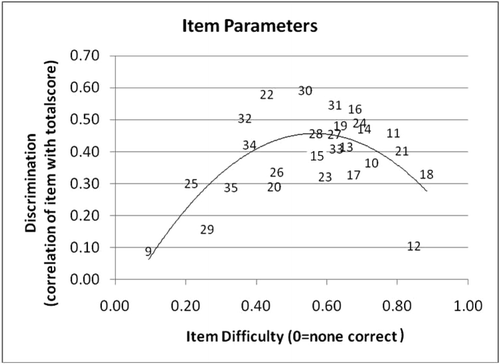
FIGURE 9: Gains for introductory and intermediate/advanced groups. Significant effect sizes are seen for all groups since each is more than 2 SE from 0.00. Treatment groups in the introductory and intermediate/advanced courses gain more than students in the Comparison groups: gains are significant for introductory groups and intermediate lab groups.

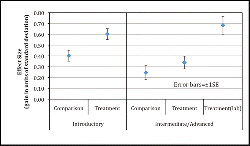
TABLE I: Number of courses and students (with matched pre- and posttests) involved in the Weather in a Tank project over 3 y.

TABLE II: Subgroups represented in the Treatment and Comparison groups (2007–2009).

TABLE III: Raw score pre- and posttest performance of study groups. For each group a standard deviation and standard error of the mean is calculated for the 27-item test. Gain is the difference between post- and pretest scores.

TABLE IV: Results from the general linear model for different groups. These two models predict student posttest scores for each of the five groups while controlling for initial pretest score, different student majors, gender, math and verbal SAT or ACT scores, and student year in college.

TABLE V: Modeled gains for each group. The expected gains for each group at each level are calculated from the general linear model, which controls for differences in student characteristics. These modeled values are somewhat different from those in Table III. Effect sizes, gain in units of standard deviation, are also reported.

TABLE VI: Sheffe tests for significant differences in gains. These tests support interpretation of significance from the overlap of error bars in Figure 9.

Notes

¹ In 2006, Marshall and Sadler sent out a questionnaire to approximately 1,000 U.S. Professors teaching Atmospheric Science to gauge their interest in the use of laboratory experiments in teaching. Of the 5% who replied, over 75% were very positive. A more detailed analysis showed that 91% are in favor of using simple laboratory experiments in class demonstrations, 55% are in favor of setting up a laboratory course, and 88% are interested in trying out some of the experiments. These findings were very encouraging, especially if interpreted in the context of the type and size of the classes taught by our targeted professors: 13% were teaching large classes (>50), 24% small classes (<20) and 63% medium classes (20–50). The survey suggests that in classes that are sufficiently large, experiments are best carried out in a demonstration mode. However, many also expressed interest in setting up hands-on laboratory courses. These broad conclusions are borne out by the Weather in a Tank project results presented here.

² See Web site http://paoc.mit.edu/labguide/projects.html for list and descriptions.

³ Students record video footage of the path of a paper dot swirling in the vortex using an overhead camera corotating with the turntable. They then track the vortex using a particle tracker that can be downloaded from the Web at http://ravela.net/particletracker.html.

⁴ In some projects we have found it useful to make use of, and encourage students to discuss, their results in the context of a 2 × 2 matrix of experiments, as discussed on the project Web site. This allows a sequence of experiments to be discussed together, in which two parameters take on two values (e.g., high and low rotation, high and low temperature gradient), yielding four experiments in all.

⁵ See, for example, the MIT Synoptic Laboratory, http://paoc.mit.edu/synoptic/ (Illari, 2001) for real time data; the NASA Earth Observatory, http://earthobservatory.nasa.gov/NaturalHazards/ for beautiful satellite images; and the COMET (UCAR), http://www.comet.ucar.edu for interesting case studies.

⁶ There were an estimated 200 unmatched test results from both the Treatment and Comparison groups that could not be identified over the 3-year period (e.g. missing date of birth [used in matching] or dates of birth that could not be matched; pretests, but no posttests, etc.).

⁷ The relationship of difficulty and discrimination is simply a product of the mathematical computation of each. To be a “perfect” discriminator, the top half of students answer correctly and the bottom half of students answer incorrectly.

⁸ Item difficulty in this figure is more accurately defined as proportion of students answering correctly.