Figures & data
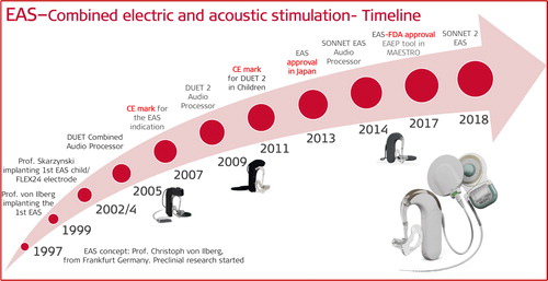
Figure 1. Morphology of inner-hair cells in three different conditions (A) [Citation2]. Typical audiogram of a partially deaf patient with severe to profound HL in the HF region: indication from the earlier times when the functional LF residual hearing cut-off was kept at 500 Hz which was extended to 1,500Hz under expanded indication criteria (indication 2) (B). Image (A) reproduced by permission of www.davidsonhearingaids.com.
![Figure 1. Morphology of inner-hair cells in three different conditions (A) [Citation2]. Typical audiogram of a partially deaf patient with severe to profound HL in the HF region: indication from the earlier times when the functional LF residual hearing cut-off was kept at 500 Hz which was extended to 1,500Hz under expanded indication criteria (indication 2) (B). Image (A) reproduced by permission of www.davidsonhearingaids.com.](/cms/asset/a31ad5fa-2c11-4ed2-9def-3fc0847e1ced/ioto_a_1888477_f0001_c.jpg)
Figure 2. Schematic representation of electric stimulation in the HF region and acoustic amplification in the LF region in an average-sized cochlea (image courtesy of MED-EL).
Figure 3. Prof. Christoph von Ilberg, Head of the ENT department, from Johann Wolfgang Goethe University Hospital Frankfurt, Germany, the inventor of the EAS concept. US patent number: 6231604B1.
Figure 4. Responses of an HF single fibre (18.1 kHz) in a normal-hearing subject during different stimulation conditions. (a) Response areas evoked by acoustic stimulation, recorded before EAS (ASb): 0 dB equals to approximately 110 dB sound pressure level (SPL). (b) Same stimulation after combined EAS (Asa). (C) Subtraction plot of acoustically evoked response areas (ASb–Asa): no differences appear. (d) Response area evoked under EAS. (e) Subtraction plot of response areas (AS–EAS). (f) Subtraction plot of response areas (EAS–AS) [Citation4]. Reproduced by permission of Karger AG, Basel.
![Figure 4. Responses of an HF single fibre (18.1 kHz) in a normal-hearing subject during different stimulation conditions. (a) Response areas evoked by acoustic stimulation, recorded before EAS (ASb): 0 dB equals to approximately 110 dB sound pressure level (SPL). (b) Same stimulation after combined EAS (Asa). (C) Subtraction plot of acoustically evoked response areas (ASb–Asa): no differences appear. (d) Response area evoked under EAS. (e) Subtraction plot of response areas (AS–EAS). (f) Subtraction plot of response areas (EAS–AS) [Citation4]. Reproduced by permission of Karger AG, Basel.](/cms/asset/7f7d56e2-140e-4651-bda4-bca1224d250e/ioto_a_1888477_f0004_c.jpg)
Figure 5. CAP audiograms in normal-hearing non-human subjects before and after chronic electric stimulation: square points refer to the time before stimulation, triangle points refer to the time shortly after the onset of stimulation, and circle points refer to 85 days after stimulation, for both stimulated and the control ear. No major differences were identified between the two ears [Citation4]. Reproduced by permission of Karger AG, Basel.
![Figure 5. CAP audiograms in normal-hearing non-human subjects before and after chronic electric stimulation: square points refer to the time before stimulation, triangle points refer to the time shortly after the onset of stimulation, and circle points refer to 85 days after stimulation, for both stimulated and the control ear. No major differences were identified between the two ears [Citation4]. Reproduced by permission of Karger AG, Basel.](/cms/asset/ab45382f-7e63-4b34-be1a-f8713c0b08be/ioto_a_1888477_f0005_b.jpg)
Table 1. Acute results of the speech understanding (Göttingen sentence test) in a single patient with LF residual hearing after CI implantation [Citation4].
Figure 6. Preoperative Freiburg monosyllabic word scores, tested with the ipsilateral HA and in the best-aided condition at optimal loudness. Postoperative monosyllabic word score with CI alone at 70 dB presentation level, and with CI + HA in the ipsilateral ear (n = 4), as well as CI + HA in the optimal condition—either ipsi-, contra-, or bi-lateral at 70 dB. Histogram created from the data given in Kiefer et al. [Citation5].
![Figure 6. Preoperative Freiburg monosyllabic word scores, tested with the ipsilateral HA and in the best-aided condition at optimal loudness. Postoperative monosyllabic word score with CI alone at 70 dB presentation level, and with CI + HA in the ipsilateral ear (n = 4), as well as CI + HA in the optimal condition—either ipsi-, contra-, or bi-lateral at 70 dB. Histogram created from the data given in Kiefer et al. [Citation5].](/cms/asset/e2f263a8-6076-4997-85f6-9fbc52d44198/ioto_a_1888477_f0006_b.jpg)
Figure 7. Clinicians from the Warsaw Institute of Physiology and Pathology of Hearing, Poland, treated the first Polish EAS-indicated patient with MED-EL device. Results of monosyllabic speech understanding after CI in quiet surroundings and noise [Citation6].
![Figure 7. Clinicians from the Warsaw Institute of Physiology and Pathology of Hearing, Poland, treated the first Polish EAS-indicated patient with MED-EL device. Results of monosyllabic speech understanding after CI in quiet surroundings and noise [Citation6].](/cms/asset/127cdc5d-fc27-48d7-914c-b5b44cd89cc2/ioto_a_1888477_f0007_c.jpg)
Figure 8. Illustration of STANDARD electrode array with apical double-lined channels and FLEX24™ electrode array with apical single-lined channels (image courtesy of MED-EL).
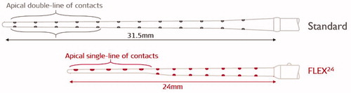
Figure 9. CI surgeons from 1 Johann Wolfgang Goethe University Hospital Frankfurt, Germany, and 2 Medical University of Vienna, Austria, who implanted MED-EL EAS™ device in patients with measurable LF residual hearing.

Figure 10. Individual audiograms and mean values (bold black line) with pre-op and three months post-op pure-tone thresholds in the ear chosen for implantation [Citation8]. Reproduced by permission of Taylor and Francis Group.
![Figure 10. Individual audiograms and mean values (bold black line) with pre-op and three months post-op pure-tone thresholds in the ear chosen for implantation [Citation8]. Reproduced by permission of Taylor and Francis Group.](/cms/asset/1f3e6cee-ce2d-4ae3-9c93-20433568d3d6/ioto_a_1888477_f0010_c.jpg)
Figure 11. Prof. Oliver Adunka from Johann Wolfgang Goethe University Hospital Frankfurt, Germany, performed an in-vitro evaluation of FLEX24™ electrode array in the year 2004.
Figure 12. Force measurement data is showing 40% lower values for FLEX24™ electrode array in comparison with the STANDARD electrode array (A) (Courtesy of MED-EL). Mean ST volume compared against STANDARD and FLEX24™ electrode arrays—a later finding from the year 2020 (B) [Citation11]. Histological evaluation of FLEX24™ in human cochlea, showing complete ST placement (C) [Citation9]. Histological image—Courtesy of Freiburg Medical University, Germany, Study sponsored by MED-EL.
![Figure 12. Force measurement data is showing 40% lower values for FLEX24™ electrode array in comparison with the STANDARD electrode array (A) (Courtesy of MED-EL). Mean ST volume compared against STANDARD and FLEX24™ electrode arrays—a later finding from the year 2020 (B) [Citation11]. Histological evaluation of FLEX24™ in human cochlea, showing complete ST placement (C) [Citation9]. Histological image—Courtesy of Freiburg Medical University, Germany, Study sponsored by MED-EL.](/cms/asset/126dbee4-1da5-42f6-9ceb-57f0d63d4d5a/ioto_a_1888477_f0012_c.jpg)
Figure 13. Engineers from MED-EL who were part of the development of DUET™ unified audio processor.
Figure 14. DUET™ unified audio processor (image courtesy of MED-EL).
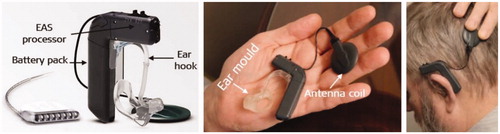
Figure 15. Mean audiograms for the implanted ear in three different listening conditions (unaided, HA alone from DUET™, and CI + HA) (A). Pruszewicz monosyllable test results in quiet at 10- and 0-dB SNR and Polish HSM sentence test results at 10 dB SNR for the group of partially deaf patients (n = 11). Mean values for the conditions DUET™ only (CI + HA), DUET™ HA only, CI only, and best-aided (plus contralateral ear) are shown with W (word test) and S (sentence test) (B). Comparison of Pruszewich monosyllable test results for three groups of patients: (1) CI patients (n = 22) tested with their CI (contralateral ear was unplugged), (2) partially deaf patients using the EAS™ (n = 11) (tested in three conditions: CI only (contralateral ear plugged), DUET™ only (contralateral ear plugged), and best-aided (plus contralateral ear)), and (3) NH group (n = 20) tested in both ears. The red shaded area shows the hearing performance gap between EAS™ and normal hearing, and the grey shaded area shows the hearing performance gap between the CI and EAS™ (C) [Citation12]. Statistical analysis: ANOVA single-factor test was used to compare speech data between three groups (p < .05). Graphs and histogram created from raw data provided by Dr Polak (MED-EL) one of the authors of Lorens et al. [Citation12].
![Figure 15. Mean audiograms for the implanted ear in three different listening conditions (unaided, HA alone from DUET™, and CI + HA) (A). Pruszewicz monosyllable test results in quiet at 10- and 0-dB SNR and Polish HSM sentence test results at 10 dB SNR for the group of partially deaf patients (n = 11). Mean values for the conditions DUET™ only (CI + HA), DUET™ HA only, CI only, and best-aided (plus contralateral ear) are shown with W (word test) and S (sentence test) (B). Comparison of Pruszewich monosyllable test results for three groups of patients: (1) CI patients (n = 22) tested with their CI (contralateral ear was unplugged), (2) partially deaf patients using the EAS™ (n = 11) (tested in three conditions: CI only (contralateral ear plugged), DUET™ only (contralateral ear plugged), and best-aided (plus contralateral ear)), and (3) NH group (n = 20) tested in both ears. The red shaded area shows the hearing performance gap between EAS™ and normal hearing, and the grey shaded area shows the hearing performance gap between the CI and EAS™ (C) [Citation12]. Statistical analysis: ANOVA single-factor test was used to compare speech data between three groups (p < .05). Graphs and histogram created from raw data provided by Dr Polak (MED-EL) one of the authors of Lorens et al. [Citation12].](/cms/asset/a2b117a3-e035-4b10-8300-61cc9971a99b/ioto_a_1888477_f0015_c.jpg)
Figure 16. A team of ENT surgeons and audiologist from Johann Wolfgang Goethe University Hospital Frankfurt, Germany, evaluated the effectiveness of DUET™ audio processor.
Figure 17. Mean results of Freiburg monosyllables in quiet at 70 dB (A), HSM sentences at 70 dB with + 10 dB SNR (B), HSM sentences at 70 dB with +5dB SNR (C), and HSM sentences at 70 dB with 0 dB SNR (D). Statistical analysis: Parametric Student’s t-test was used to detect discrepancies between the test intervals (p < .05). Histogram created from data given in Helbig et al. [Citation13].
![Figure 17. Mean results of Freiburg monosyllables in quiet at 70 dB (A), HSM sentences at 70 dB with + 10 dB SNR (B), HSM sentences at 70 dB with +5dB SNR (C), and HSM sentences at 70 dB with 0 dB SNR (D). Statistical analysis: Parametric Student’s t-test was used to detect discrepancies between the test intervals (p < .05). Histogram created from data given in Helbig et al. [Citation13].](/cms/asset/1cd23310-a2a1-4d0e-b74b-2ab170cf1517/ioto_a_1888477_f0017_c.jpg)
Figure 18. Mean pure-tone audiometric results of DUET™ users (n = 11) and DUET™ nonusers (n = 4) (A). Speech audiometry results of the four patients who rejected DUET™ and used the CI processor: the Freiburg monosyllable word test correct answers with 66% (mean) (B) and HSM sentence correct answers with 62% at 10 dB SNR (mean) (C). Graph and histograms created from data given in Helbig et al. [Citation14].
![Figure 18. Mean pure-tone audiometric results of DUET™ users (n = 11) and DUET™ nonusers (n = 4) (A). Speech audiometry results of the four patients who rejected DUET™ and used the CI processor: the Freiburg monosyllable word test correct answers with 66% (mean) (B) and HSM sentence correct answers with 62% at 10 dB SNR (mean) (C). Graph and histograms created from data given in Helbig et al. [Citation14].](/cms/asset/0e408f10-2f9d-45aa-880a-e91d921ebbe0/ioto_a_1888477_f0018_c.jpg)
Figure 19. DUET-2™ EAS™ audio processor with its remote control FineTuner™ (image courtesy of MED-EL).
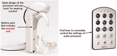
Figure 20. Mean Pruszewicz monosyllabic word recognition in background noise with an SNR of +10dB (A) and mean subjective report on sound quality satisfaction of music stimuli (B) [Citation15]. Statistical tests: One-way repeated measures (RM) ANOVAs were used to assess the improvement of DUET™ and DUET-2™ and the level of user satisfaction across three-time intervals. Reproduced by permission of Taylor and Francis Group.
![Figure 20. Mean Pruszewicz monosyllabic word recognition in background noise with an SNR of +10dB (A) and mean subjective report on sound quality satisfaction of music stimuli (B) [Citation15]. Statistical tests: One-way repeated measures (RM) ANOVAs were used to assess the improvement of DUET™ and DUET-2™ and the level of user satisfaction across three-time intervals. Reproduced by permission of Taylor and Francis Group.](/cms/asset/e414bc7b-18b3-44f9-89ee-17a56d2c1866/ioto_a_1888477_f0020_b.jpg)
Figure 21. Instrument identification. Scores on instrument identification according to instruments for all three groups. Histogram created from data given in Brockmeier et al. [Citation16].
![Figure 21. Instrument identification. Scores on instrument identification according to instruments for all three groups. Histogram created from data given in Brockmeier et al. [Citation16].](/cms/asset/b4fdb34c-ea90-44ea-89f2-68dc8f4939fa/ioto_a_1888477_f0021_c.jpg)
Figure 22. Preoperative and postoperative audiograms showing the mean hearing level for each frequency for the CI implanted group (A). Monosyllable scores overtime under the noisy condition for patients with PD. Graph and histogram created from data given in Skarzynski et al. [Citation18].
![Figure 22. Preoperative and postoperative audiograms showing the mean hearing level for each frequency for the CI implanted group (A). Monosyllable scores overtime under the noisy condition for patients with PD. Graph and histogram created from data given in Skarzynski et al. [Citation18].](/cms/asset/3f3d7b3f-5b82-4fc8-a5d7-b40b40702a9e/ioto_a_1888477_f0022_c.jpg)
Figure 23. FLEX28™ electrode array with an implantable array length of 28 mm, along with five apical channels in a single line and extra slim configuration (Image courtesy of MED-EL).
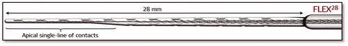
Figure 24. First report on hearing preservation after reimplantation by Dr Ronald Hoffman from New York Eye and Ear Infirmary, New York, USA.
Figure 25. CI surgeons from the University of Western Australia (in 2012) reported on hearing preservation after CI reimplantation surgery.

Figure 26. Pure-tone audiometry results of case 1 (child) and case 2 (adult) with pre-op (grey line), post-1-year CI (black line) and post-re-implantation (red line) audiogram results [Citation21]. Reproduced by permission of Wolters Kluwer Health, Inc.
![Figure 26. Pure-tone audiometry results of case 1 (child) and case 2 (adult) with pre-op (grey line), post-1-year CI (black line) and post-re-implantation (red line) audiogram results [Citation21]. Reproduced by permission of Wolters Kluwer Health, Inc.](/cms/asset/671f4d44-1428-4dff-b6e8-6be183060cdf/ioto_a_1888477_f0026_c.jpg)
Table 2. Demographic data of the three patients with preserved residual hearing after undergoing reimplantation [Citation22].
Figure 27. Pure-tone audiometric thresholds determined preoperatively and postoperatively in three patients, implanted with EAS™ [Citation22]. Reproduced by permission of Wolters Kluwer Health, Inc.
![Figure 27. Pure-tone audiometric thresholds determined preoperatively and postoperatively in three patients, implanted with EAS™ [Citation22]. Reproduced by permission of Wolters Kluwer Health, Inc.](/cms/asset/d37763ef-c634-4474-970c-55bb40c1266b/ioto_a_1888477_f0027_c.jpg)
Figure 28. Unaided pure-tone audiometric hearing thresholds at various time points, including at the device failure time point, and three months post-reimplantation (A). Speech perception test results at various time points (B). Graph and histogram created from data given in Thompson et al. [Citation23].
![Figure 28. Unaided pure-tone audiometric hearing thresholds at various time points, including at the device failure time point, and three months post-reimplantation (A). Speech perception test results at various time points (B). Graph and histogram created from data given in Thompson et al. [Citation23].](/cms/asset/520186fd-9709-45ca-b199-f610d21d7fae/ioto_a_1888477_f0028_b.jpg)
Table 3. Scale for the proposed hearing preservation classification system [Citation24].
Table 4. Clinicians from the HEARRING group who were involved in establishing the method of HP classification.
Figure 29. Team of clinicians from USA (1Vanderbilt University, 2Arizona State University, 3Mayo Clinic, Rochester, 4University of Texas Southwestern, 5University of North Carolina), Poland (6International Center for Hearing and Speech) and 7MED-EL demonstrated the benefits of binaural hearing by preserving the LF residual hearing during CI procedure in the ipsilateral ear.
Figure 30. Individual and mean speech recognition scores (% correct) for fixed level SNR of +6dB and +2dB for both groups under two different listening conditions and the participant numbers inside the red boxes correspond to MED-EL implanted devices (A). The Polish group given under +2dB SNR was actually tested at 0 dB SNR as per the personal communication from the authors. Normalised EAS benefit for speech recognition at +6dB and +2dB SNR as a function of low-frequency pure-tone average in dB HL (note: Polish group was tested at 0 dB SNR and not at +2dB SNR as mentioned in this study, according to the personal communication from the authors) (B) [Citation25]. Reproduced by permission of Wolters Kluwer, Inc.
![Figure 30. Individual and mean speech recognition scores (% correct) for fixed level SNR of +6dB and +2dB for both groups under two different listening conditions and the participant numbers inside the red boxes correspond to MED-EL implanted devices (A). The Polish group given under +2dB SNR was actually tested at 0 dB SNR as per the personal communication from the authors. Normalised EAS benefit for speech recognition at +6dB and +2dB SNR as a function of low-frequency pure-tone average in dB HL (note: Polish group was tested at 0 dB SNR and not at +2dB SNR as mentioned in this study, according to the personal communication from the authors) (B) [Citation25]. Reproduced by permission of Wolters Kluwer, Inc.](/cms/asset/712eb44e-3517-48d7-aa86-8af68a36a480/ioto_a_1888477_f0030_c.jpg)
Figure 31. SONNET® EAS™ audio processor (image courtesy of MED-EL).
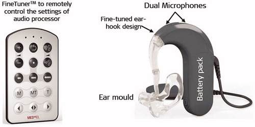
Figure 32. Team of CI surgeons from Japan: 1Shinshu University School of Medicine, 2Toranomon Hospital, Tokyo, 3Kobe City Medical Center General Hospital, 4Nagasaki University Graduate School of Biomedical Sciences, and 5Miyazaki University School of Medicine were involved in the clinical evaluation of EAS™ hearing system.
Figure 33. Pure-tone audiograms of each of the twenty-nine operated ears measured at various time points. Black continuous lines correspond to the preoperative time points and the red continuous lines correspond to the twelfth month post-surgery. Shadow indicates the audiological criteria for EAS clinical trial. The average audiogram of all ears is shown within the red outlined section [Citation27]. Reproduced by permission of Taylor and Francis Group.
![Figure 33. Pure-tone audiograms of each of the twenty-nine operated ears measured at various time points. Black continuous lines correspond to the preoperative time points and the red continuous lines correspond to the twelfth month post-surgery. Shadow indicates the audiological criteria for EAS clinical trial. The average audiogram of all ears is shown within the red outlined section [Citation27]. Reproduced by permission of Taylor and Francis Group.](/cms/asset/c2b3cd84-2702-4a37-8db9-92621b44d87b/ioto_a_1888477_f0033_c.jpg)
Figure 34. Mean values for speech discrimination and perception scores at different time points and under different listening conditions [Citation27]. Monosyllable word test in quiet (A), in noise (+10dB SNR) (B), word test in noise (+10dB SNR) (C), and sentence test in noise (+10dB SNR) (D). Statistical analysis: paired t-test. Reproduced by permission of Taylor and Francis Group.
![Figure 34. Mean values for speech discrimination and perception scores at different time points and under different listening conditions [Citation27]. Monosyllable word test in quiet (A), in noise (+10dB SNR) (B), word test in noise (+10dB SNR) (C), and sentence test in noise (+10dB SNR) (D). Statistical analysis: paired t-test. Reproduced by permission of Taylor and Francis Group.](/cms/asset/6794efe7-de8e-4fcf-ab8c-aa52a996967f/ioto_a_1888477_f0034_b.jpg)
Figure 35. Clinicians from CI clinics across the USA who were involved in the FDA clinical trial study evaluating the safety and effectiveness of MED-EL EAS™ system. 1University of North Carolina, 2Kansas University Medical Center, 3Hospital of the University of Pennsylvania, 4Miller School of Medicine of the University of Miami, 5Medical College of Wisconsin, 6Stanford University, 7New York Eye and Ear Infirmary, 8Duke University, 9University of Texas Southwestern Medical Center, 10Indiana University, 11Swedish Neuroscience Institute, 12Oregon Health Sciences University, 13Michigan University, 14Boys Town National Research Hospital, Nebraska and 15MED-EL.
Figure 36. Average pure-tone unaided thresholds. Lines show mean audiograms obtained preoperatively (grey, solid line, diamonds), at three months (grey, long-dashed line, circles), at six months (grey, short-dash line, stars) and twelve months post-activation (black line, triangles). Error bars indicating standard deviation from the mean are shown for pre-op and twelve months interval (A). Speech recognition scores for all patients followed-up until the twelfth-month post-activation interval. Scores for CUNY sentences in noise (B) and CNC words in quiet (C) are represented by filled circles for patients using EAS and open triangles for those tested in CI alone condition. A solid reference line is shown on both figures, indicating no change in score from the preoperative to the twelfth-month post-activation interval. Dashed lines are shown at ±10% of the solid reference line to indicate scores that may fall within test-retest variability [Citation28]. Statistical analysis: paired t-tests and Wilcoxon signed-rank test, with least-square means used to estimate change from the preoperative interval. Reproduced by permission of Wolter Kluwer Health, Inc.
![Figure 36. Average pure-tone unaided thresholds. Lines show mean audiograms obtained preoperatively (grey, solid line, diamonds), at three months (grey, long-dashed line, circles), at six months (grey, short-dash line, stars) and twelve months post-activation (black line, triangles). Error bars indicating standard deviation from the mean are shown for pre-op and twelve months interval (A). Speech recognition scores for all patients followed-up until the twelfth-month post-activation interval. Scores for CUNY sentences in noise (B) and CNC words in quiet (C) are represented by filled circles for patients using EAS and open triangles for those tested in CI alone condition. A solid reference line is shown on both figures, indicating no change in score from the preoperative to the twelfth-month post-activation interval. Dashed lines are shown at ±10% of the solid reference line to indicate scores that may fall within test-retest variability [Citation28]. Statistical analysis: paired t-tests and Wilcoxon signed-rank test, with least-square means used to estimate change from the preoperative interval. Reproduced by permission of Wolter Kluwer Health, Inc.](/cms/asset/abf850ee-ee71-4907-ab2e-08742d5309e7/ioto_a_1888477_f0036_b.jpg)
Table 5. Summary of primary and secondary effectiveness endpoints.
Table 6. Summary of primary outcomes (CNC word scores) comparing MED-EL EAS and Cochlear Hybrid hearing system.
Figure 37. FLEXSOFT™ electrode array with its dimensions in millimetres (image courtesy of MED-EL). Mean pure-tone audiograms measured at three different time points [Citation31]. Statistical analysis: Nonparametric Wilcoxon signed-rank test to look for the difference between test intervals (p < .05). Reproduced by permission of Wolters Kluwer Health, Inc.
![Figure 37. FLEXSOFT™ electrode array with its dimensions in millimetres (image courtesy of MED-EL). Mean pure-tone audiograms measured at three different time points [Citation31]. Statistical analysis: Nonparametric Wilcoxon signed-rank test to look for the difference between test intervals (p < .05). Reproduced by permission of Wolters Kluwer Health, Inc.](/cms/asset/dd295262-a5ea-46f5-881c-6b14981b726a/ioto_a_1888477_f0037_b.jpg)
Figure 38. Prof. Marcus Atlas studied the long-term HP results from his patient population implanted with MED-EL EAS™ system. Results are summarised in the above graph: hearing preservation over time and the linear trendline summarises changes over time—statistical analysis: 1-way ANOVA test. Histogram created from the data given in Santa-Maria et al. [Citation31].
![Figure 38. Prof. Marcus Atlas studied the long-term HP results from his patient population implanted with MED-EL EAS™ system. Results are summarised in the above graph: hearing preservation over time and the linear trendline summarises changes over time—statistical analysis: 1-way ANOVA test. Histogram created from the data given in Santa-Maria et al. [Citation31].](/cms/asset/f865d187-ca89-466a-a436-9732364aecc9/ioto_a_1888477_f0038_c.jpg)
Figure 39. Hearing preservation for each patient using the HP numerical scale [Citation33]. Reproduced by permission of Wolters Kluwer Health, Inc.
![Figure 39. Hearing preservation for each patient using the HP numerical scale [Citation33]. Reproduced by permission of Wolters Kluwer Health, Inc.](/cms/asset/27fc0f33-ef86-452c-aa28-82793ba1819a/ioto_a_1888477_f0039_b.jpg)
Figure 40. The linear regression coefficient for the decline in HP score of the stable hearing group, as categorised from the average linear regression coefficient of the decrease in hearing preservation score (A). The linear regression coefficient for the decline in HP score of the progressive HL group (B) [Citation34]. The dotted line in black in both graphs, indicates the average for the contralateral ear. Reproduced by permission of Taylor and Francis Group.
![Figure 40. The linear regression coefficient for the decline in HP score of the stable hearing group, as categorised from the average linear regression coefficient of the decrease in hearing preservation score (A). The linear regression coefficient for the decline in HP score of the progressive HL group (B) [Citation34]. The dotted line in black in both graphs, indicates the average for the contralateral ear. Reproduced by permission of Taylor and Francis Group.](/cms/asset/3d593568-5692-41c3-86a4-8020a7f3462c/ioto_a_1888477_f0040_c.jpg)
Figure 41. HP with regards to shifts of pure-tone averages in low frequencies (125-, 250- and 500-Hz). Results are shown for postoperative, 12 months, and long-term shifts (>24 months) from pre-operative measurement. Histogram created from data given in Helbig et al. [Citation35].
![Figure 41. HP with regards to shifts of pure-tone averages in low frequencies (125-, 250- and 500-Hz). Results are shown for postoperative, 12 months, and long-term shifts (>24 months) from pre-operative measurement. Histogram created from data given in Helbig et al. [Citation35].](/cms/asset/0ec195a4-5c3d-4fd3-95af-ce91c283c47a/ioto_a_1888477_f0041_c.jpg)
Figure 42. Clinicians from University Clinic St. Pölten, Austria, who investigated the long-term HP in EAS™ CI users.
Table 7. Eight patients (ten ears) with long-term follow-up data [Citation36].
Figure 43. Speech results of all patients with the DUET™ fitting parameters [Citation40]. CI = electric only; HA = acoustic only; DUET = EAS; (image courtesy of Dr Polak from MED-EL).
![Figure 43. Speech results of all patients with the DUET™ fitting parameters [Citation40]. CI = electric only; HA = acoustic only; DUET = EAS; (image courtesy of Dr Polak from MED-EL).](/cms/asset/1d7ff2a3-f5a4-4823-b6eb-fca26f919d69/ioto_a_1888477_f0043_c.jpg)
Table 8. Recommended age-specific assessment tools. [Citation44].
Figure 44. ENT surgeon from New York, USA, and engineers from MED-EL established the mathematical function in the estimation of patient-specific CDL.
Figure 45. Mathematical equations to estimate the CDL along the organ of Corti (Image courtesy of MED-EL).
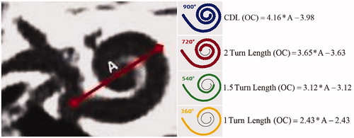
Figure 46. Applying the CDL value in Greenwood’s frequency function would result in patient-individual frequency map. From this map, the starting point of LF residual hearing is possible to identify (image courtesy of MED-EL) [Citation49].
![Figure 46. Applying the CDL value in Greenwood’s frequency function would result in patient-individual frequency map. From this map, the starting point of LF residual hearing is possible to identify (image courtesy of MED-EL) [Citation49].](/cms/asset/99e3109e-b0b0-49ff-b5b0-23aa22ff5979/ioto_a_1888477_f0046_c.jpg)
Figure 47. Illustration of Greenwood’s frequency map for an average CDL of 35 mm with an assumption of low frequency functional residual hearing, starting at 1,000Hz. Visualisation of different electrode array lengths shows how many channels would be in the acoustic amplification zone (image courtesy of MED-EL).
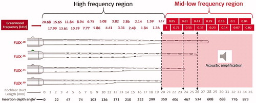
Figure 48. Example audiogram of pre-op (open-circle) and post-op (crossed circle) with the MEDIUM performed with a MED-EL STANDARD electrode array. The HP remained stable over eighteen months (A). Effect of electrode insertion depth on postoperative change in hearing (B). Using the RW approach, there was no clear relationship between implant insertion depth and post-operative PTA [Citation50]. Reproduced by permission of Journal of American Academy of Audiology.
![Figure 48. Example audiogram of pre-op (open-circle) and post-op (crossed circle) with the MEDIUM performed with a MED-EL STANDARD electrode array. The HP remained stable over eighteen months (A). Effect of electrode insertion depth on postoperative change in hearing (B). Using the RW approach, there was no clear relationship between implant insertion depth and post-operative PTA [Citation50]. Reproduced by permission of Journal of American Academy of Audiology.](/cms/asset/e3fbd54e-79b2-4e21-a8ef-32c35153ffcb/ioto_a_1888477_f0048_b.jpg)
Figure 49. Mean audiograms of the implanted ear at four testing time points (pre-op and post-op at 3, 6, and 13 months). Error bars depict standard deviations [Citation51]. Statistical test: ANOVA two-factor-without-replication test was used for comparison of hearing thresholds at various time points (p < .05). Reproduced by permission of Taylor and Francis Group.
![Figure 49. Mean audiograms of the implanted ear at four testing time points (pre-op and post-op at 3, 6, and 13 months). Error bars depict standard deviations [Citation51]. Statistical test: ANOVA two-factor-without-replication test was used for comparison of hearing thresholds at various time points (p < .05). Reproduced by permission of Taylor and Francis Group.](/cms/asset/a1ef7f0e-7814-4398-b9a9-5da2b4a65c34/ioto_a_1888477_f0049_c.jpg)
Figure 50. Air-conducted hearing thresholds at 6 months postactivation for 16 mm insertion (n = 3) and 20 mm insertion (n = 3) [Citation54]. Reproduced by permission of Wolters Kluwer Health, Inc.
![Figure 50. Air-conducted hearing thresholds at 6 months postactivation for 16 mm insertion (n = 3) and 20 mm insertion (n = 3) [Citation54]. Reproduced by permission of Wolters Kluwer Health, Inc.](/cms/asset/1136194e-8246-4426-9197-c9f1bef34a58/ioto_a_1888477_f0050_b.jpg)
Figure 51. Average air-conduction hearing thresholds. The dashed and solid lines indicate pre-op and six months post-op, respectively. Grey and black lines show the individual and mean results [Citation43]. Reproduced by permission of Taylor and Francis Group.
![Figure 51. Average air-conduction hearing thresholds. The dashed and solid lines indicate pre-op and six months post-op, respectively. Grey and black lines show the individual and mean results [Citation43]. Reproduced by permission of Taylor and Francis Group.](/cms/asset/cecaf72b-2d90-4ba5-b8d7-85c89f9d7d8d/ioto_a_1888477_f0051_c.jpg)
Figure 52. Prof. Oliver Adunka, who led the study in characterizing ECoghG signals. Example comparison of extracochlear (at the RW membrane) and intracochlear (just over the RW membrane) ECochG recordings [Citation57]. Reproduced by permission of Wolters Kluwer Health, Inc.
![Figure 52. Prof. Oliver Adunka, who led the study in characterizing ECoghG signals. Example comparison of extracochlear (at the RW membrane) and intracochlear (just over the RW membrane) ECochG recordings [Citation57]. Reproduced by permission of Wolters Kluwer Health, Inc.](/cms/asset/e39861f1-ff38-4c42-bf41-8bae31399e69/ioto_a_1888477_f0052_b.jpg)
Figure 53. Prof. Gunesh Rajan was the first one to measure CM during CI procedure. Post-op CM measurements (from the top) at intra-op, and ten days, three weeks, three months, and six months post-op [Citation59]. Reproduced by permission of Wolters Kluwer Health, Inc.
![Figure 53. Prof. Gunesh Rajan was the first one to measure CM during CI procedure. Post-op CM measurements (from the top) at intra-op, and ten days, three weeks, three months, and six months post-op [Citation59]. Reproduced by permission of Wolters Kluwer Health, Inc.](/cms/asset/10abbe53-6fc4-45df-8bea-4671efd9e10f/ioto_a_1888477_f0053_c.jpg)
Figure 54. Prof. Artur Lorens led the study in measuring CM directly from the CI during CI surgery. Example of intracochlear ECochG recordings for tone pips and clicks from electrode channels 1, 3, and 5 [Citation56].
![Figure 54. Prof. Artur Lorens led the study in measuring CM directly from the CI during CI surgery. Example of intracochlear ECochG recordings for tone pips and clicks from electrode channels 1, 3, and 5 [Citation56].](/cms/asset/c5fc8559-7377-4b08-b0bf-8653518cc031/ioto_a_1888477_f0054_c.jpg)
Figure 55. Clinicians from Hannover Medical School. Example of an intraoperative ECochG recording just after the electrode insertion process. Data is shown for 1,000Hz tone burst [Citation59]. Image courtesy of Dr Sabine Haumann, Hannover, Germany.
![Figure 55. Clinicians from Hannover Medical School. Example of an intraoperative ECochG recording just after the electrode insertion process. Data is shown for 1,000Hz tone burst [Citation59]. Image courtesy of Dr Sabine Haumann, Hannover, Germany.](/cms/asset/eb37a7b1-4738-4943-88b9-dd0d4c8848a8/ioto_a_1888477_f0055_c.jpg)
Figure 56. Aetiology of patients with residual acoustic hearing. (A) (n = 41): orange indicates genetic causes of HL; yellow indicates other causes; grey indicates unknown. (B): comparison of HP scores in each group [Citation19]. Reproduced by permission of Taylor and Francis Group.
![Figure 56. Aetiology of patients with residual acoustic hearing. (A) (n = 41): orange indicates genetic causes of HL; yellow indicates other causes; grey indicates unknown. (B): comparison of HP scores in each group [Citation19]. Reproduced by permission of Taylor and Francis Group.](/cms/asset/11c97bec-27c9-4a00-a6b5-1e557965cea6/ioto_a_1888477_f0056_c.jpg)
Figure 57. Clinicians from two biggest Hospital in Beijing, China, who undertook the concurrent hearing and genetic screening of 180,469 neonates with follow-up.

Figure 58. Clinicians from the Institute of Physiology and Pathology of Hearing, Warsaw who introduced the Electro-Natural Stimulation in partial deafness treatment of adults CI users.
Figure 59. Average pre-op and post-op air conduction hearing thresholds for operated and non-operated ear [Citation62]. Reproduced by permission of Karger AG, Basel.
![Figure 59. Average pre-op and post-op air conduction hearing thresholds for operated and non-operated ear [Citation62]. Reproduced by permission of Karger AG, Basel.](/cms/asset/8a7cb27e-7647-4da5-9eea-756f26feab65/ioto_a_1888477_f0059_c.jpg)
Figure 60. Clinicians from around the world who have hosted the HSP meeting between 2002–19. 1Indiana University, USA; 2Johann Wolfgang Goethe University Hospital Frankfurt, Germany; 3UT Southwestern Medical Center, USA; 4Institute of Physiology and Pathology of Hearing, Poland; 5University of North Carolina, USA; 6Antwerp Medical University, Belgium; 7Kansas University Medical Center, USA; 8Medical University of Vienna, Austria; 9University of Miami Ear Institute, USA; 10 St. Thomas Hospital, UK; 11Sunnybrook Health Sciences Centre, Canada; 12Heidelberg Medical University, Germany; 13Shinshu University, Japan; 14Vanderbilt University, USA; 15University Hospital of North Paris, France; 16University of Western Australia, Australia; 17Uppsala University, Sweden; 18New York Eye and Ear Infirmary, USA.
Figure 61. Experts from MED-EL, who are responsible for the HSP workshop, logistically supported by MED-EL.