Figures & data
Figure 1. Diagrams of in situ hydrolysis reaction and injection protocol. Upon injection, the DCA-Cl undergoes hydrolysis in the kidney (a). The exothermic reaction produces dichloroacetic acid and HCl and releases -93 kJ/mol of energy. Additionally, a diagram shows the injection sequence (b). The dose of the reactive aliquot, in red, is varied with nonselective or selective injection. DCA-Cl: dichloroacetyl chloride; HCl: hydrochloric acid; kJ: kilojoule; l: liter; mol: mole.
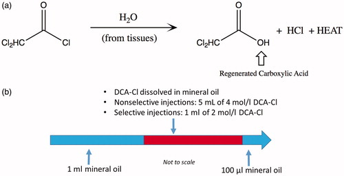
Table 1. Summary of experiments and corresponding Figures.
Figure 2. Experimental setup and gross pathology at 24 h. The experimental setup of the kidney and reference vials is shown before a thermoembolization experiment (a). The renal artery is cannulated with a catheter (a). The gross pathology of a nonselective injection experiment is demonstrated in (b), 24 h post-injection. 24 h after injection, gross pathology images for the two selective injection experiments are shown in (c) and (d). (c) shows a bivalve kidney whereas surface damage is visible in (d).
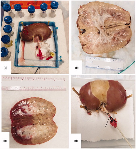
Figure 3. MRTI vs. thermal probe. Left (a) is a coronal T1-weighted image of the kidney before injection, surrounded by the reference vials. The blue arrow indicates the location of the thermal probe in the renal cortex. Right (b) compares the temperature probe data (black line) with a spatially-matched 2 × 2 voxel region of interest (ROI) from the MRTI (green). The plotted ROI temperature (b) data in has ±2σ error bars where σ is the standard deviation of temperature of a 10 × 10 voxel region of a reference vial, at each time point. The location of the noise ROI is at the red square (a). MRTI: magnetic resonance thermal imaging; ROI: region-of-interest; and σ: standard deviation.
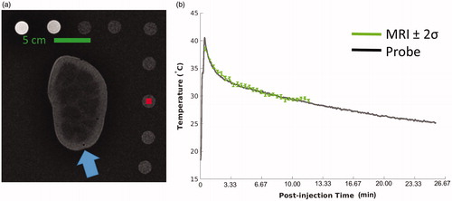
Table 2. Comparison of MRTI and fiber optic temperature probe data.
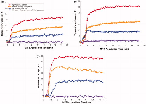
Figure 4. Selected ROI locations. MRTI data are shown from the three experiments with homogeneous baseline temperatures. Each image is a coronal temperature map of the kidney after injection, at a late time point and has three colored circles (indicated by white arrows) denoting the locations of three 2 × 2 voxel ROIs. The ROI temperature histories are plotted in , and ROI points are color-matched to the data points of . The surrounding reference vials are cropped. MRTI: magnetic resonance temperature imaging; ROI: region-of-interest.
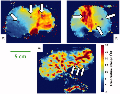
Figure 5. Time elapsed MRTI. From an experiment with a homogeneous baseline temperature, a single coronal slice demonstrates the time evolution of temperature. Every other time frame image is displayed to simplify presentation. The heating is diffuse initially at 1.5 min. Heating intensifies in the small vessels of the renal cortex, during the interval of 2.2–4.5 min. Finally, heating appears in the larger upstream vessels extending proximally back toward the main renal artery, at 5.2 min and later. MRTI: magnetic resonance thermal imaging.
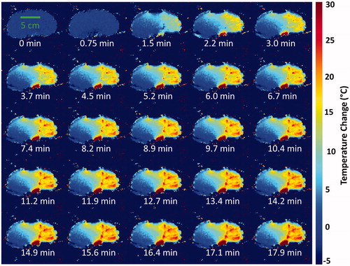
Figure 6. Comparison of CT and MRTI. The pre- (a) and 45-min post-injection (b) CT images of a selective injection experiment are juxtaposed. Both coronal reformatted CT images are inverted grayscale minimum intensity projections that are 5 mm thick. Window/level settings are 168/33. The CT minimum intensity projection and intensity inversion depict the post-injection presence of the mineral oil associated with the heating indicated on MRTI. CT: Computed tomography; MRTI: magnetic resonance thermal imaging.
Figure 7. Selected ROI plots. These three plots show temperature data at the locations indicated by the color-matched ROI locations in ; an ROI is a 2 × 2 voxel region. The ROI locations of correspond with (a), etc. The purple data points are from unheated reference vials, which are cropped out of the images in . The rapid and large temperature rise is clearly shown, along with the unexpected result that cooling had not occurred at termination of data collection in each case. MRTI: magnetic resonance temperature imaging; ROI: region-of-interest.