Figures & data
Table I. Guidelines for TBI diagnosis.
Figure 1. Structural brain imaging refers to a set of procedures for measuring a variety of morphometric properties of the brain. Alterations in brain structure in individuals or groups of individuals may be linked to pathologic processes. Different types of imaging contrasts measure various aspects of brain structure including (A) T1-weighted (typically used for differentiation of gray and white matter and cortical surface modeling), (B) T2-weighted (typically used to detect tissue pathology with increased fluid content), and (C) Fluid attenuated inversion recovery (FLAIR; typically used to measure pathology including stroke). The pial and white matter surfaces are outlined in yellow and green, respectively, capturing the thickness of the cortex. Aberrations in each scan can represent neural abnormalities such as white matter lesions (red arrow) or hemosiderins (orange arrow).
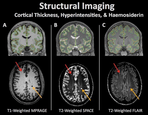
Figure 2. Cortical thickness in structural imaging is a measurement of the distance from the grey-white matter boundary (green outline) to the edge of the cortex, or pial surface (yellow outline). Cortical thickness can change with normal aging as well as pathology. An example of a single subject is shown on the right with yellow regions demonstrating the areas with the highest cortical thickness and thinner regions of the cortex in red.
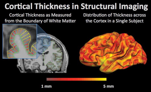
Figure 3. Computational procedures can be used to model the brain and to measure the structural properties of brain tissue within defined regions. The figure demonstrates the automated (A) parcellation of the cerebral cortex based on gyral anatomy and (B) segmentation of subcortical regions by the FreeSurfer software suite (freesurfer.net). The amount of tissue in the different regions is typically compared between groups to determine regional vulnerability to degenerative processes.
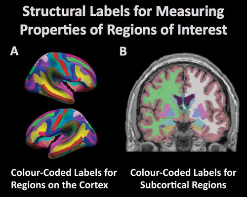
Figure 4. Diffusion weighted imaging refers to a set of magnetic resonance imaging procedures that exploit water diffusion in tissue as the basis of image contrast. Diffusion imaging measures various properties of the behavior of water in the brain such as fractional anisotropy (FA), radial diffusivity, etc. These measurements can be used to quantify various aspects of tissue microstructure, which can be compared between groups, as well as used in visualization of the anatomy of prominent white matter fascicles and other anatomical properties. (A) The white matter tracts of a single subject’s brain, reconstructed from the FA values where high FA represents regions of strict, directed water diffusion (along the borders of white matter bundles) and low FA indicates regions with isotropic water diffusion. (B) The white matter tracts from FA values are color-coded to indicate the direction of water diffusion in order to illustrate the arrangement and organization of bundles of white matter. (C) Visualization of diffusion tensor imaging (DTI) data in the axial (left), sagittal (top right), and coronal plane (bottom right). Fiber bundle directionality is indicated by color (red = right to left/left to right (e.g. corpus callosum), green = posterior to anterior/anterior to posterior (e.g. cingulum bundle), blue = inferior to superior/superior to inferior (e.g. corticospinal tracts)).
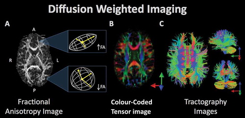
Figure 5. Task-related fMRI refers to the use of MRI to measure regional brain responses to cognitive and/or behavioral stimulation. (A) In the fMRI paradigm, an experimental task is performed at known times during imaging, and the resulting expected brain response (measured by MRI as the ‘hemodynamic response’ due to the phenomenon of neurovascular coupling) can be statistically analyzed to determine regions of the brain supporting the operations used to perform the task. (B) Activation patterns associated with behavioral fluctuations during a sustained attention task in 145 veterans from the TRACTS cohort (image courtesy of Dr. Michael Esterman, VA Boston Healthcare System).
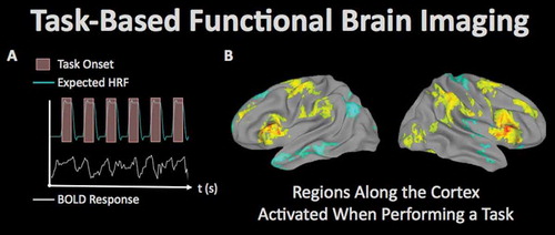
Figure 6. Functional connectivity refers to procedures used to examine covariance in regional brain activity. Correlated activity across brain regions is interpreted to indicate shared demands for a cognitive operation between regions, and potentially direct communication between regions. The image demonstrates a ‘seed’ region in the posterior cingulate (top) in which the fMRI signal (based on the blood oxygenation level-dependent mechanism of contrast) is quantified across time (blue waveform) and correlated with other regions throughout the brain. This analysis highlights functional connectivity among a set of regions referred to as the ‘default mode network,’ which has been demonstrated to be compromised across a range of conditions including blast exposure [Citation73]. The red-yellow regions demonstrate positive correlation to the seed in which the fMRI signal is quantified across time (green waveform) and plotted over the fMRI signal from the seed (middle). The positive correlation between these two time-series is plotted in yellow (middle right). The blue-light blue regions demonstrate anticorrelation to the seed in which the fMRI signal is quantified across time (red waveform) and plotted over the fMRI signal from the seed. The anticorrelation between these two time-series is plotted in light blue (bottom right).
![Figure 6. Functional connectivity refers to procedures used to examine covariance in regional brain activity. Correlated activity across brain regions is interpreted to indicate shared demands for a cognitive operation between regions, and potentially direct communication between regions. The image demonstrates a ‘seed’ region in the posterior cingulate (top) in which the fMRI signal (based on the blood oxygenation level-dependent mechanism of contrast) is quantified across time (blue waveform) and correlated with other regions throughout the brain. This analysis highlights functional connectivity among a set of regions referred to as the ‘default mode network,’ which has been demonstrated to be compromised across a range of conditions including blast exposure [Citation73]. The red-yellow regions demonstrate positive correlation to the seed in which the fMRI signal is quantified across time (green waveform) and plotted over the fMRI signal from the seed (middle). The positive correlation between these two time-series is plotted in yellow (middle right). The blue-light blue regions demonstrate anticorrelation to the seed in which the fMRI signal is quantified across time (red waveform) and plotted over the fMRI signal from the seed. The anticorrelation between these two time-series is plotted in light blue (bottom right).](/cms/asset/b148e5d3-6750-4a08-add5-abef6f4acd58/ibij_a_1327672_f0006_oc.jpg)
Figure 7. Electrophysiological activity in the brain can be evaluated using electroencephalography (EEG) and magnetoencephalography (MEG). These techniques measure changes in the electric and magnetic fields, respectively, which are presumed to originate in the brain sources and rapidly propagate toward the participants’ scalp, affording high temporal resolution of the recordings. Event-related data can elucidate neural processing during performance on a task, discerning differences typically lasting between 50 and 500 ms. Top-left shows time-courses of the average electrophysiological response evoked by stimuli from two conditions (40 trials per condition) at FC1 and P5 EEG sensors positioned on the scalp (by convention negative voltages are plotted up). The scalp topography at the time-points (indicated by white arrows), when the between-condition differences were maximal at each of these electrodes, is shown in top-right (the data from 64 EEG sensors, locations of FC1 and P5 sensors indicated by the black dot). The fronto-central effect shown in blue (the time-course displayed in blue is more negative) and the left-posterior effect shown in red (the time-course displayed in yellow is more negative) peaked approximately 50 ms apart and were likely generated by distinct neural sources. Models can be estimated that localize EEG and MEG data, recorded at the scalp, to the neural sources. Bottom-left shows time-courses of the average evoked electrophysiological activity (60 trials per condition) estimated at the cortical regions shown in bottom-right. The time-course in the experimental condition shown in yellow peaked a few dozens of ms earlier in the left temporal cortex (TC) than in the left prefrontal cortex (PFC).
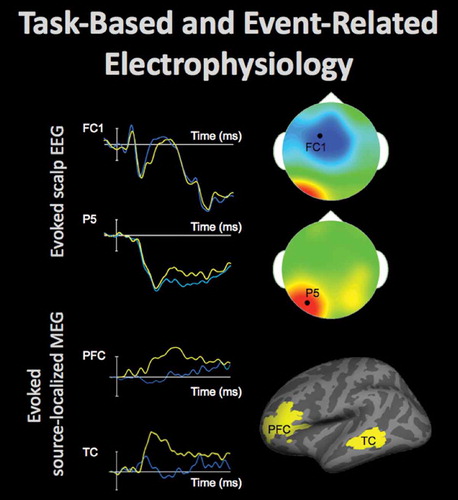
Figure 8. High temporal resolution of EEG/MEG, combined with an acceptable spatial resolution (on the order of 10 mm) of the source-localized activity estimates, afford dynamic information on connectivity in the large-scale functional neural networks, which is complementary to the fMRI data. Amplitude fluctuations in the band-limited electrophysiological oscillations (e.g. in the 15–30 Hz beta band) can be measured in regions of interest (ROIs), such as areas in the inferior-parietal cortex (IPC) and temporal cortex (TC) shown in top-left, by taking an absolute value of the Hilbert-transformed data, as shown in top-right (oscillating activity time-course is shown in blue, and the Hilbert-transformed amplitude-envelope is shown in red). Then, functional connectivity between the ROIs can be evaluated by computing a correlation between the amplitude-envelope time-courses, as shown for the TC and IPC envelopes in bottom-left (yellow dots show the corresponding time-point data). The functional connectivity between ROIs may be dynamic as is evident from the values of the correlation between the ROI envelope time-courses, which may vary over time, as shown in bottom-right for IPC (red) and TC (blue) time-courses: for approx. 10 seconds the correlation was close to zero, but for the next approx. 10 seconds-long time-interval the correlation increased to 0.61.
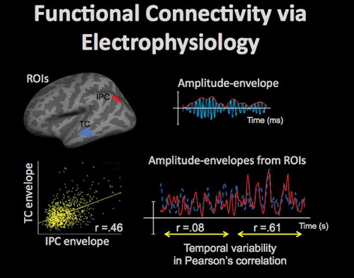
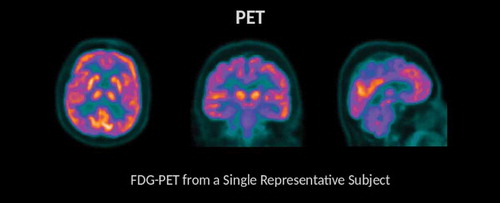
Figure 9. FDG-PET is a procedure that provides information about energy utilization in the brain. This is achieved through the use of an injected radiolabeled analog of glucose (FDG). Given that glucose is a primary energy substrate in the brain, FDG accumulation within brain areas is a marker of metabolic activity and this measure of energetics is regionally diminished in a variety of clinical conditions. Brighter colors are found in regions with greater tracer uptake (and therefore greater metabolic activity).