The formation and use of hierarchical cognitive maps in the brain: A neural network model

Figures & data

Figure 1. The figure shows the architecture of the proposed hierarchical neural network model. The current state of the agent is input by the state cells (State) and the goal of the agent is input by the goal cells (Goal). Actions that moves the agent towards its goal are produced by the co-operation of the state-action cells (State Action) and the sequence cells (Sequence). Finally, the planned action is read out by the gating cells (Gate) and propagated to the action cells (Action), which produce movement

Figure 2. The pattern of connectivity between SA Cells encoding a reverse causal model. All SA cells within a given column encode the same state, and each SA cell encodes a different state-action combination. We hypothesize that each SA cell should receive a set of afferent synapses from all of the SA cells encoding its predicted successor state, allowing cells in a successor state to activate the SA cell responsible for entering that successor state. Likewise, each SA cell sends an efferent synapse to any SA cells that will result in the SA cell’s own encoded state

Figure 3. Illustration of the problem of reading out the correct action for the current state. (a) shows the firing rates of a layer of SA cells partway through a planning task. Each compass plot in (a) represents the firing rate of all SA cells which encode a particular state as illustrated in (b). The golden state is the goal location and the boxed state is the agent’s current state. The planning wavefront has activated a large number of SA cells, most of which encode an action (NW, SW, W) that will not move the agent towards the goal. The model cannot therefore simply sum or average the activity in the SA layer but has to gate this activity by the current state of the agent before it is passed to the action output layer. Furthermore, this read-out must happen at a specific time

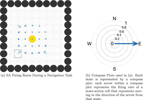
Figure 4. The Gating Problem. This figure shows compass plots of state-action activity during planning at three different times T = 3, 6 and 11. If the agent is occupying the state marked by the square, then the model should only read out activity from the SA cells marked by the square, and not (for example) those marked by crosses. Also, the agent should not read out activity from the marked SA cells at t = 3 (when the wave of activity has not yet reached the agent’s state) or at t = 11 (when the wave of activity has passed the agent’s state) but only at t = 6

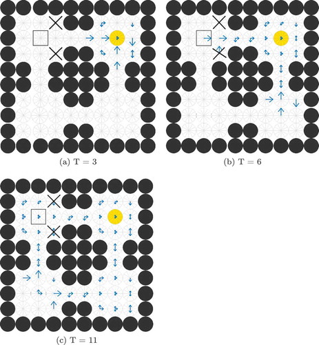
Figure 5. The 2-dimensional grid-world state space used to test the simulated network agents. The agent can move between blue squares, which are free states, and cannot move into yellow squares, which are walls. Each state has a unique index value which is used to fire a specific state cell

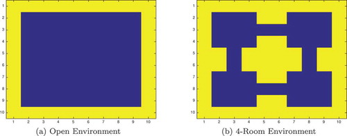
Table 1. Table of parameters for the hardwired model with sequence cells described in Section 3

Parameter	Value
Action Cell Threshold t^A$t^A$	0.2
Gating Cell Threshold t^G$t^G$	0.55

Figure 6. This figure shows the propagation of activity from the goal location through the SA layer during a simulated navigation task in the four-room environment shown in Figure 5(b). Results are shown for simulations with and without sequence cells. Each state is represented by a compass plot which depicts the activity of the SA cells representing that state (see Figure 3(b)). The golden state represents the goal, and the boxed state represents the agent’s current location. The agent moves once activity reaches its current state. We see that activity propagates considerably faster when sequence cells are available – compare (a) vs (b) – and that the propagating activity therefore reaches considerably more states after five timesteps

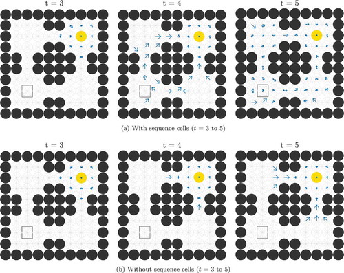
Figure 7. A figure showing how the total planning time varies with navigation tasks whose solutions are of different lengths. Results are shown for open environments as illustrated in Figure 5(a) (left column) and 4-room mazes illustrated in Figure 5(b) (right column). This demonstrates that use of sequences in planning produces low efficiency benefits during short tasks but increasingly large benefits as the required route length increases

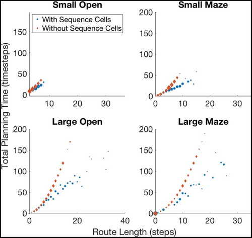
Figure 8. Fitting curves to the results of navigating within Large Open environments. The basic model, without using sequences, produces planning times that increase quadratically with the route length, while the augmented model, using sequences, plans linearly with the route length. Extrapolating these fits predicts that the gains should grow very large as the size and complexity of environments increase, although we cannot currently verify this claim as the discrete state-action representation we use does not scale well beyond 20 × 20 states (discussed further in Sec. 6.1). To check the accuracy of both fits, we have calculated the Adjusted-$R^2$ values for each fit. The Adjusted-$R^2$ is a statistical measure of how close the data are to the fitted lines, adjusted for the number of terms that describe the fitted line. These values are 1 for the model without sequence cells and 0.9243 for the model with sequence cells. The value of Adjusted-$R^2$ must be between 0 and 1, and so these values show that both lines fit the data extremely well

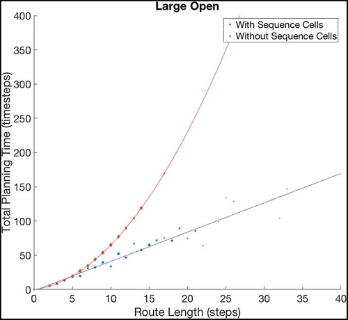
Figure 9. Two Gate Environment (8x8). As in Figure 5, the agent can move between blue squares, which are free states, and cannot move into yellow states, which are walls. The green square represents the goal, and the red square represents the agent’s starting state. The agent therefore starts equidistant from both gates, and can reach the goal from either gate in the same number of timesteps

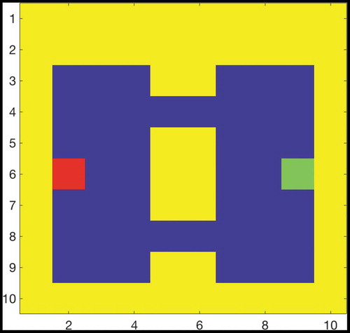
Figure 10. This figure compares the probability of an agent occupying various states in a two-gate environment (Figure 9) over the course of 100 planning trials. (a) shows these occupancy probabilities when the model has access to sequence cells that encode a route through the lower gate. (b) shows the same model without access to these cells. The agent is required to move from position (2,6) to (9,6), which can be achieved in the same number of actions by passing through either gate. We see that the existence of these sequences biases the agent to use the familiar lower gate rather than the higher gate in (a). By contrast, when the agent does not have access to these sequences it uses both gates with approximately equal probability (b)

Figure 11. Comparison of a simulated sequence cell to a recorded pre-SMA cell. In both the simulated and recorded data, we see that the cell has strong firing before but not during a specific sequence of actions (a dashed line marks the onset of this sequence). However, the simulated data displays periodicity, unlike the recorded data. This is discussed in the main text. The proposed model is rate-coded and so the raster plot (a) was generated from recorded firing rates using a Poisson distribution

Table 2. Table of parameters for the model described in Section 4.1

Parameter	Value
Action Cell to SA Cell Rescaling ($t^{A-SA}$)	0.25
State Cell to SA Cell Rescaling ($t^{S-SA}$)	1
SA Cell Upper Threshold $t_{max}^{SA}$	1.5
SA Cell Lower Threshold $t_{min}^{SA}$	0.5
Learning Rate ($k)$	100

Figure 12. Single cell information learned by SA cells in a task using overlapped distributed xy representations of the agent’s state. Maximum information is indicated by the horizontal dashed line, and the maximum number of SA cells that can form without redundancy is indicated by the vertical dashed line

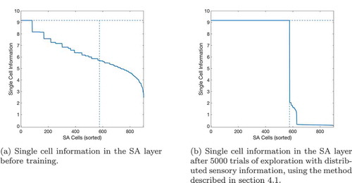
Figure 13. Firing of SA cells in a task using overlapped distributed xy representations of the agent’s state. The number of SA cells which fire for each state-action combination is recorded before and after training. (a) demonstrates that before training, a small number of SA cells will fire uniquely for one state-action combination (see also Figure 12(a)) due to the random initial synaptic connectivity between state cells, action cells and SA cells. A few state-action combinations are therefore uniquely represented by one SA cell before training. (b) then shows that after training, all state-action combinations are uniquely represented by one SA cell

Figure 14. This figure records how many states (Figure 14(a)) and SA combinations (Figure 14(b)) are encountered when the agent is allowed to explore for different numbers of timesteps. It shows that the agent has explored more than half of an open 10 by 10 state map after ^~100 timesteps and almost every possible state after ^~500 timesteps

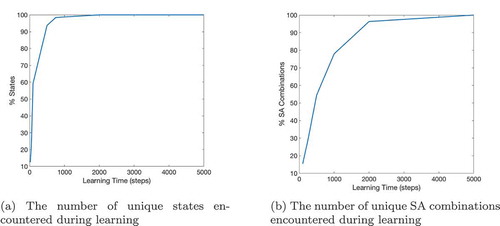
Figure 15. Network architecture for learning a cognitive map in the recurrent connections between self-organizing SA cells

Table 3. Table of parameters for self-organizing model incorporating layer of SA cells described in Section 4.2

Parameter	Value
Input Learning Rate ($k^{IN})$	100
Trace Learning Rate ($k^{RC}$)	10

Figure 16. This figure shows the precision and recall achieved by the self-organizing columnar SA model described in Section 4.2. This model was run for 5000 timesteps of exploration in an open 8 × 8 environment. Precision and recall can vary between 0 and 1, and are plotted here as percentages. We observe that both precision and recall are at 100%. The model is able to represent all of the true transitions existing in the environment, and represents them all correctly

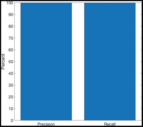
Figure 17. Architecture of the proposed model with self-organizing gating layer

Table 4. Table of model parameters for Section 4.3

Parameter	Value
Gating Cell Upper Threshold $t_{max}^G$	1.5
Gating Cell Lower Threshold $t_{min}^G$	0.5
Gate Learning Rate ($k^G)$	100

Figure 18. Single cell information analysis of gating cells after learning. A horizontal dashed line indicates the maximum possible information that a gating cell can encode. This is calculated as ${log}_2\left(N_{ST}{N}_{SA}\right)$, where $N_{ST}$ is the number of available states and $N_{SA}$ is the total number of SA cells. A vertical dashed line indicates the maximum number of gating cells that can self-organize; this is effectively equal to $N_{ST}{N}_A$ where $N_A$ is the number of available actions (9). This is because there are only $N_{ST}{N}_A$ legitimate combinations of state and SA in any environment that a simulated agent can experience, since the state represented by the state cells must always be the same state as represented by the SA cells during exploration. We see that in both experiments, the maximum number of gating cells that can self-organize have learned to encode the maximum possible single-cell information

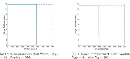
Figure 19. The number of gating cells that encode each state-SA combination before and after training. Figure 19(a) shows that no gating cell fires uniquely for any combination of state and SA cells before the exploration period. Figure 19(b) shows that after training, gating cells fire uniquely for certain combinations of state and SA cells. Unlike the equivalent figure (Figure 13) in Sec. 4.1, which shows that at least one SA cell responds uniquely to every state-action combination after training, there is not a unique gating cell for every state and SA combination. This is because an SA cell (which encodes a unique combination of state and action) will only fire in conjunction with its associated state during exploration. Most state and SA cell combinations are therefore invalid: the cells in the gating layer will never experience this combination of inputs. We have therefore sorted the x-axis so that the valid state and SA cell combinations, which the agent can actually experience, lie along a diagonal, and we see that one gating cell has learned to respond to each of these valid combinations. Figure 19(c) zooms in on this diagonal (from Figure 19(b)) and shows that there are in fact several valid state-SA combinations for each state cell. This is because a number of SA cells exist for each state, each representing a different action in that state. We see that a gating cell fires uniquely for all of the state-SA combinations available for each state

Figure 20. Efferent synaptic connectivity of gating cells after self-organization in an 8 × 8 open environment using the method described in Section 4.3. The x-axis shows the postsynaptic action cells, and the y-axis shows the presynaptic gating cells. For clarity, the y-axis has been sorted so that cells with a strong efferent connection to a particular action cell are grouped together. We see that the majority of gating cells (specifically $N_{ST}{N}_A$ = 576) form a strong synapse to one and only one action cell. This is what we expect: as in Figure 18(a) the maximum number of gating cells that can self-organize is 576, and these cells have also formed strong efferent connections to action cells, allowing them to pass on activity to the action cells and so produce action output as in Sec. 3

Figure 21. The percentage of successful trials if the model explores for a certain number of timesteps during training and is then used (instead of a hardwired model) to perform planning tasks identical to those in Section 3

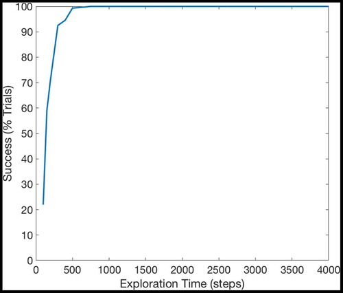
Figure 22. The percentage of SA combinations that the model has experienced after a certain number of timesteps. The model explores randomly, and so as its knowledge of the map grows more comprehensive, it becomes less likely to experience unknown SA combinations. The amount of environmental knowledge that the model contains therefore increases very quickly during early exploration but it takes many timesteps for the model’s knowledge of the environment to become comprehensive

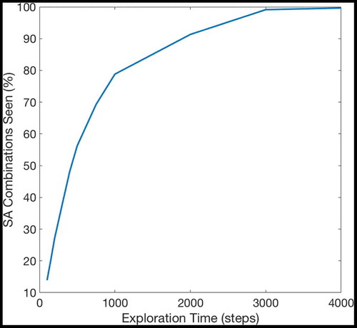
Figure 23. The probability that an agent will take the lower gate in the “normal” and “reduced” conditions, based on 100 trials in each condition. In the normal condition, the SA to SA weights encoding a transition through the lower gate (see Figure 9 for the structure of the two-gate environment) are kept at their original value of 0.44. The synaptic weights for both gates are therefore equal, and so the agent takes each path with approximately equal (50%) probability. In the reduced condition, the synaptic weights associated with the lower gate are reduced to 10% of their original value. Under the probabilistic planning paradigm described in Sec. 4.4, activation has a significantly lower probability of passing through the lower gate in any given timestep due to the reduced synaptic weights encoding this transition and therefore the agent is much less likely to pass through the lower gate. Note that the likelihood of taking either path depends on the ratio between the synapses encoding transitions through each gate and not on the absolute value of these synapses

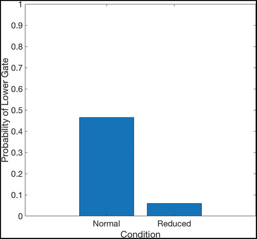
Figure 24. The maze used in the Tolman & Honzig detour task, in which rats navigate through a maze to a food box (Martinet et al. 2011). The maze consists of three pathways (Path 1, Path 2 and Path 3) with different lengths. A block can be introduced at point A (preventing the rat from navigating through Path 1), or point B (preventing the rat from navigating through Path 1 or 2). A gate near the second intersection prevents rats from going right to left. This figure is reproduced from Martinet et. al. 2011 (Martinet et al. 2011) in accordance with the Creative Commons Attribution (CC BY) licence

Figure 25. Occupancy grids for Tolman & Honzig detour task. The occupancy grids show the probability that a modelled agent will at some point pass through each section of the maze during the various trial types. The scale runs from 0 to 1. An occupancy of 1 means that every agent passed through that point during every trial of that type; an occupancy of zero shows that no agent ever passed through that point in any trial of that type. We see that in the majority of Open trials, the agent takes the shortest possible route to the goal: the direct Path 1. In the majority of trials where Path 1 is blocked at Point A, the agent takes the now-shortest Path 2. Finally, in the majority of trials where Paths 1 and 2 are blocked at Point B, the agent takes the now-shortest Path 3. The qualitiative performance of both the Martinet model and the proposed model is similar

Figure 26. Comparison of model output to previous experimental and modelling results. Each box plot shows the distribution of route choices over trials of a particular type (Open, Blocked A or Blocked B). (a) shows experimental results from rats. (b) shows the results of the proposed model. The chosen path in each trial is recorded by measuring the last section of maze that the agent moves through before it reaches the goal

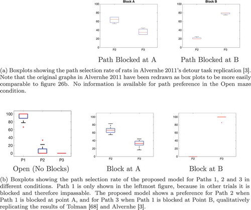
Table 5. Table of parameters for the learning of sequence cells as described in Section 5

Parameter	Value
Trace Constant Eta $\eta$	0.5
Sequence Cells to SA Cells Learning Rate ($k^{SQ-SA}$)	11
SA Cells to Sequence Cells Learning Rate ($k^{SA-SQ}$)	${10}^{26}$
SA Cells to Sequence Cells Threshold ($t^{SA-SQ}$)	$0.1$

Figure 27. Examples of two learned sequences. The magnitude of each arrow represents the weight of the synapse from the sequence cell to that SA cell (left column) or the weight of the synapse to the sequence cell from that SA cell (right column). Synapses have been normalized so that 1 is the maximum synapse. We see that the weight structure is consistent with that described in Section 3, with sequence cells receiving synapses only from the last SA cell in a sequence (b, d) and sending synapses to all SA cells in that sequence (a, c). See Figure 3(b) for legend

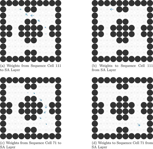
Figure 28. Success rates in planning task when using learned sequences. This figure shows the percentage success rates of the network in 100 trials

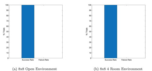
Figure 29. The occupation of different states during the sequence-learning period. (a) shows the probability of an agent occupying any given state in this 4-room environment (Figure 5) while (b) shows the number of sequences associated with each state after 300 planning tasks in this environment. By comparing the two, we see that states that are occupied more often have more associated sequences. This strongly suggests that the model tends to learn sequences that are “useful”, in other words sequences that occur frequently in the solutions to planning tasks that take place in this environment

Martinet L-E, Sheynikhovich D, Benchenane K, Arleo A. 2011. Spatial learning and action planning in a prefrontal cortical network model. PLoS Comput Biol. 70(5):e1002045. doi:10.1371/journal.pcbi.1002045.

 Google Scholar