Semi-empirical model for timber truck speed profile and fuel consumption

Figures & data

Table 1. Test fleet composition. “Axles” refers to the number of axles on the truck and the trailer, respectively. In general, maximum allowed gross vehicle weight for combinations with 7, 8, and 9 axles are 64 tonnes, 70 tonnes, and 74 tonnes.

Vehicle	Truck	Model year	Power (kW)	Axles	Trailer tires	Loader
1	Volvo FH 64R	2018	552	3+4	dual	fixed
2	Scania R580b	2020	427	3+5	dual	fixed
3	Volvo FH13	2018	405	3+5	dual	fixed
4	Scania R580b	2018	427	3+4	dual	detachable
5	Volvo FH 64R	2019	405	3+4	dual	separate loader
6	Scania R580b	2019	427	3+4	dual	separate loader
7	Scania R580b	2018	427	4+4	single	separate loader
8	Scania R580b	2018	427	4+4	dual	separate loader
9	Volvo FH 64R	2018	405	3+5	dual	detachable
10	Volvo F16	2015	375	4+4	single	separate loader
11	Scania 650	2019	478	4+5	single	separate loader
12	Volvo FH16	2020	552	4+5	dual	separate loader
13	Scania 650	2019	478	4+5	single	detachable
14	Volvo FH16	2019	552	4+5	dual	separate loader
15	Scania 650	2018	478	4+5	dual	separate loader
16	Scania R580b	2018	427	3+4	dual	detachable
17	Scania R520b	2016	382	3+4	dual	detachable
18	Volvo FH13	2016	405	3+5	dual	detachable
19	Volvo FH16	2016	552	3+5	dual	detachable
20	Scania R730b	2021	537	4+5	dual	separate loader
21	Volvo FH16	2020	552	4+5	dual	detachable

Table 2. Symbols used for the behavior model.

Symbol	Meaning	Typical values	Unit
$v^{\lim }$	Speed limit	8–22	ms^−1
$v^{\mathrm{curve}}$	Highest speed with respect to horizontal curvature. Determined statistically.	1.0–22	ms^−1
$v^{\mathrm{rdw}}$	Highest speed with respect to road width. Determined statistically.	5–22	ms^−1
$v^{\mathrm{vis}}$	Highest speed with respect to visibility.	variable	ms^−1
$v^{\mathrm{cls}}$	Highest speed with respect to road class. Determined statistically.	11–22	ms^−1
$a^{\max }$	Acceleration. Limited by engine power, speed, gross weight, road gradient, traction and driver comfort. Determined statistically but physically limited.	0.0–0.5 (Can be negative for steep climbs.)	ms^−2
$a^{\min }$	Deceleration. Mainly determined by economical driving. Determined statistically.	−0.6–0.0	ms^−2
$a^{\mathrm{lov}}$	Deceleration at sudden loss of visibility. Value according to Swedish Road Administration (2015).	−1.0	ms^−2
$a^{\mathrm{em}}$	Highest emergency deceleration. Value according to Swedish Road Administration (2015).	−2.0	ms^−2
$\mathit{S}$	Line of sight. Calculated.	>10	m
$\mathit{R}$	Curve radius. From NVDB.	>10	m

Table 3. Deceleration depending on speed. Intervals in kmh⁻¹ and deceleration in ms⁻². (intervals do not include their right end point.)

Season	Speed interval
	0–<5	5–<15	15–<25	25–<35	35–<45	45–<55	55–<65	65–<75	75–<85	85–<95
	Loaded vehicle
winter	−0.32	−0.33	−0.38	−0.39	−0.32	−0.26	−0.22	−0.19	−0.15	−0.12
summer	−0.35	−0.41	−0.42	−0.45	−0.37	−0.29	−0.24	−0.20	−0.16	−0.13
	Unloaded vehicle
winter	−0.34	−0.39	−0.46	−0.52	−0.46	−0.38	−0.31	−0.26	−0.20	−0.15
summer	−0.37	−0.44	−0.48	−0.56	−0.52	−0.43	−0.35	−0.29	−0.22	−0.17

Table 4. Acceleration depending on speed. Intervals in kmh⁻¹ and acceleration in ms⁻² (intervals do not include their right end point.).

	Speed interval
	0–<5	5–<15	15–<25	25–<35	35–<45	45–<55	55–<65	65–<75	75–<85	85–<95
	Loaded vehicle
winter	0.31	0.26	0.29	0.29	0.25	0.21	0.18	0.16	0.13	0.12
summer	0.35	0.31	0.32	0.31	0.27	0.22	0.19	0.17	0.14	0.12
	Unloaded vehicle
winter	0.35	0.33	0.36	0.41	0.39	0.33	0.29	0.24	0.17	0.13
summer	0.40	0.39	0.38	0.44	0.43	0.37	0.33	0.28	0.19	0.13

Figure 1. Relationship between curvature and speed for one of the vehicles when loaded and unloaded.

Figure 2. Empirical relationship between curvature and maximum speed during winter and spring when loaded and unloaded. Also indicated is the dependency according to a formula used by the Swedish Road Administration (2004).

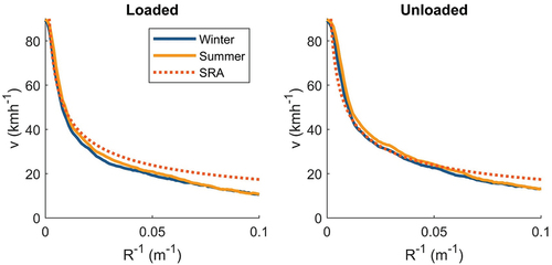
Figure 3. Maximum speed depending on road width when loaded and unloaded.

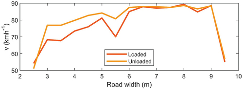
Figure 4. Relationship between speed and functional road class when loaded and unloaded.

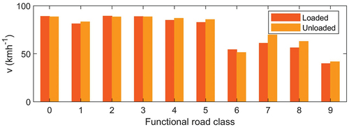
Figure 5. Simulated speed profile and the influence of visibility.

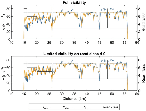
Table 5. Symbols used for the vehicle response model.

Symbol	Meaning	Typical values	Unit
$C_r$	Coefficient of rolling resistance	0.006	-
$C_d$	Coefficient of air drag	0.8	-
$F_{\mathit{rr}}$	Rolling resistance force	1–5	kN
$\mathit{A}$	Frontal area	10.4	m^2
$\mathit{N}$	Normal force	variable	N
$\mathit{m}$	Gross weight	17,000–74,000	kg
$m_{\mathrm{rot}}$	Rotating mass equivalent (depends on wheel number and type)	1,550–1,950	kg
$m_{\mathrm{eff}}=\mathit{m}+m_{\mathrm{rot}}$	Effective mass	18,550–75,950	kg
$\mathit{v}$	Speed	variable	ms^−1
$\mathit{a}$	Acceleration	variable	ms^−2
$\mathit{\rho }$	Air density	1.2	kgm^−3
$\mathit{g}$	Gravitational constant	9.82	ms^−2
$\mathit{\alpha }$	Road gradient	variable	-
$\mathit{P}$	Power	0–550	kW

Table 6. Measured coefficients of rolling resistance for 15 vehicles. Values are normalized to 0 °C and a temperature sensitivity of $4.5\cdot {10}^{-5}$ per 1 °C.

Vehicle	2	3	4	5	7	8	9
$C_r$	0.0064	0.0076	0.0068	0.0064	0.0060	0.0049	0.0064
11	13	14	15	16	17	18	19
0.0067	0.0060	0.0065	0.0064	0.0068	0.0062	0.0072	0.0077

Figure 6. Chemical power demand as a function of mechanical power demand.

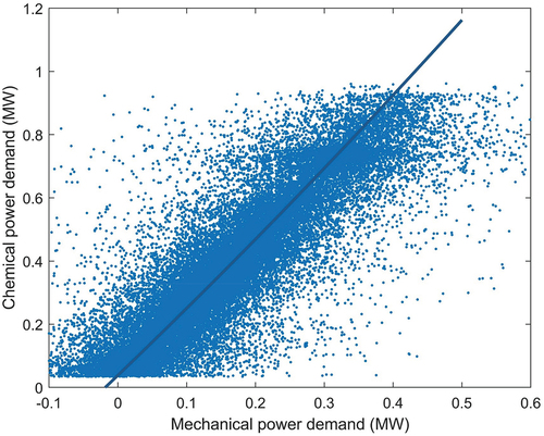
Figure 7. Speed profile of repeated driving cycle for a timber vehicle.

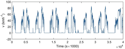
Figure 8. Comparison between real time and simulated time for a set of driving cycles during winter and summer.

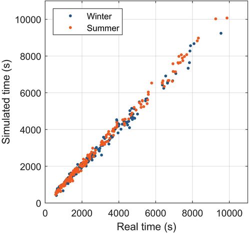
Table 7. Accuracy and precision for the driver simulator during winter and summer.

Accuracy measure	Winter	Summer
Ratio total simulated time/real time	1.010	1.038
RMS error	7.9 %	7.4 %
Avg absolute error	5.6 %	5.8 %

Figure 9. Comparison of observed and computed fuel consumption for a number of routes of varying length during winter and summer.

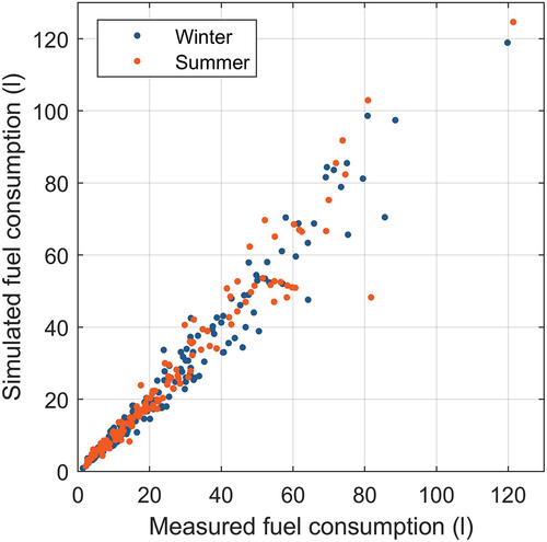
Table 8. Accuracy and precision for the fuel consumption model applied on simulated driving cycles of varying length during winter and summer.

Accuracy measure	Winter	Summer
Ratio simulated/measured fuel volume for trip	0.989	1.01
RMS error	16 %	15 %
Avg absolute error	14 %	11 %

Swedish Road Administration. 2015. Vägars och gators utformning, Begrepp och grundvärden. (Design of roads and streets. Concepts and default values.). Trafikverkets publikation 2015:090.

 Google Scholar

Swedish Road Administration. 2004. Vägar och gators utformning, Linjeföring. (Design of roads and streets. Road alignment). Vägverkets publikation 2004:80. ISSN 1401–9612.

 Google Scholar