Identification of four key biomarkers and small molecule drugs in nasopharyngeal carcinoma by weighted gene co-expression network analysis

Figures & data

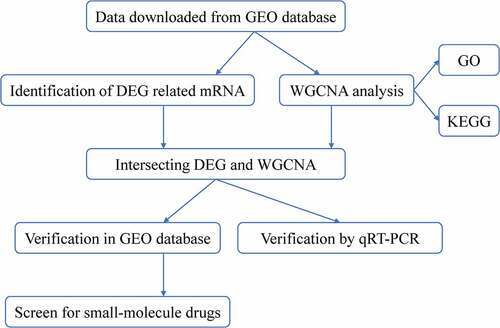
Table 1. Primers used for the qRT-PCR

MARK1	F: 5‘- GAGCGGGACACGGAAAATCAT −3’
	R: 5‘- TGCTACTCGACTTGGTAGGCT −3’
PGAP1	F: 5‘- CTTCGGCTTCGAGGAGAATAAG −3’
	R: 5‘- GGGATAGCGTTTTGCCAGTTT −3’
KITLG	F: 5‘- AATCCTCTCGTCAAAACTGAAGG −3’
	R: 5‘- CCATCTCGCTTATCCAACAATGA −3’
CRIP1	F: 5‘- TAATGACGGCCCGGTCTTTTA −3’
	R: 5‘- TGCAGCGTGCTGGGTTTAAT −3’
GAPDH	F: 5‘- TGTGGGCATCAATGGATTTGG −3’
	R: 5‘- ACACCATGTATTCCGGGTCAAT −3’

Table 2. Characteristics of datasets included in the integrated analysis

Year	Source	First author	Country	Assay type	Platform	PMID
2008	GSE12452	Ahlquist P	USA	Affymetrix Human Genome U133 Plus 2.0 Array	GPL570	22,880,099
2014	GSE53819	Qian CN	China	Agilent-014850 Whole Human Genome Microarray 4x44K	GPL6480	24,763,226
2009	GSE13597	Yap L	United Kingdom	Affymetrix Human Genome U133A Array	GPL96	19,142,888
2016	GSE40290	Huang ZX	China	Capitalbio 22 K Human oligo array version 1.0	GPL8380	NA
2017	GSE64634	Xiong W	China	Affymetrix Human Genome U133 Plus 2.0 Array	GPL570	26,246,469

Figure 1. Differentially expressed genes and common differentially expressed genes in two datasets. (a and b) The volcano plots visualize the differentially expressed genes in GSE12452 and GSE53819. (c and d) Common differentially expressed genes in two datasets

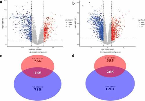
Figure 2. Determination of soft-thresholding power in the weighted gene co-expression network analysis (WGCNA). (a) Analysis of the scale-free fit index for various soft-thresholding powers (β). The red line indicates where the correlation coefficient is 0.9, and the corresponding soft-thresholding power is 5. (b) Analysis of the mean connectivity for various soft-thresholding powers. The red line indicates where the correlation coefficient is 0.9, and the corresponding soft-thresholding power is 5. (c) Histogram of connectivity distribution when β = 5. (d) Checking the scale-free topology when β = 5

Figure 3. Construction of WGCNA modules. (a) The cluster dendrogram of module eigengenes. (b) The cluster dendrogram of the genes with median absolute deviation in the top 25% in the GSE12452. Each branch in the figure represents one gene, and every color below represents one co-expression module

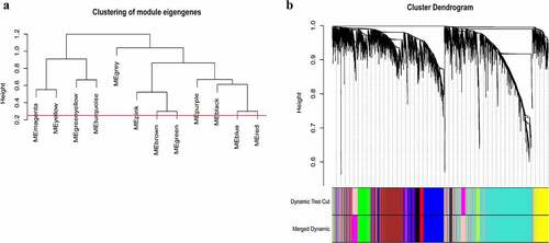
Figure 4. Relationship between modules and clinical traits. (a) Module eigengene dendrogram and eigengene network heatmap summarize the modules yielded in the clustering analysis. (b) Heatmap of the module-trait relationships. The green module was significantly associated with N stage

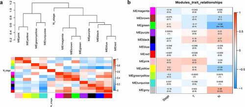
Figure 5. Functional enrichment analysis of hub module genes. (a) GO terms and KEGG pathway were presented, and each band represents one enriched term or pathway colored according to the -log10(p). (b) Network of the enriched terms and pathways. Nodes represent enriched terms or pathway with node size indicating the number of hub module genes involved in. Nodes sharing the same cluster are typically close to each other, and the thicker the edge displayed

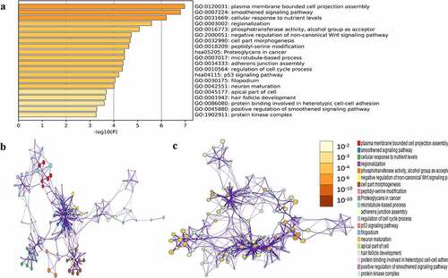
Figure 6. Identification of hub module and candidate hub gene. (a) Distribution of average gene significance and errors in the modules associated with the NPC. (b) Scatter plot for correlation between gene module membership in the green module and gene significance

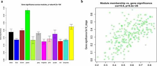
Figure 7. Validation of hub genes in the gene expression level. (a-d) Validation of hub genes in the GSE12452. PGAP1, MARK1, and KITLG were significantly higher expression in NPC compared with normal tissues, while CRIP1 was significantly lower expression in NPC compared with normal tissues. (e-h) Validation of hub genes in the GSE53819 and the results were the same as earlier

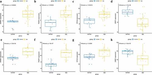
Figure 8. Validation of hub genes in the diagnostic value. (a-d) Validation of hub genes in the GSE12452. Receiver operating characteristic (ROC) curves and area under the curve (AUC) statistics are used to evaluate the capacity to discriminate NPC from normal controls with excellent sensitivity and specificity. (e-h) Validation of hub genes in the GSE53819 and the results were the similar as earlier. These findings indicated these four hub genes have excellent diagnostic efficiency in NPC

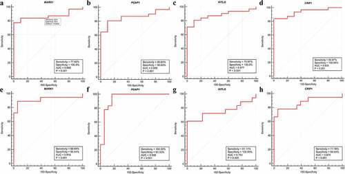
Figure 9. Validation the expression levels of four hub genes in the combined microarray datasets. (a-d) PGAP1, MARK1, and KITLG were significantly higher expression in NPC compared with normal tissues, while CRIP1 was significantly lower expression in NPC compared with normal tissues

Table 3. Top 10 most significant small molecule drugs based on CMAP

CMAP name	Mean	Number	Enrichment	P-value	Specificity	Percent non-null
vorinostat	0.369	12	0.423	0.0171	0.6181	58
pioglitazone	0.234	11	0.412	0.03326	0.2313	54
fludrocortisone	−0.265	8	−0.469	0.03975	0.3732	50
thalidomide	0.497	7	0.607	0.00501	0	71
bendroflumethiazide	0.33	6	0.598	0.01363	0.0145	50
chlorcyclizine	−0.486	6	−0.592	0.01619	0.0089	66
etiocholanolone	−0.481	6	−0.581	0.01903	0.2208	66
hyoscyamine	0.62	5	0.717	0.00411	0	100
sulfadiazine	0.667	5	0.711	0.00473	0	100
biperiden	−0.354	5	−0.674	0.00863	0.1905	60

Abbreviations: CMAP, Connectivity map.

Figure 10. Relative expression of MARK1, PGAP1, KITLG and CRIP1 mRNA in clinical nasopharyngeal carcinoma tissues and cell lines. (a-d) The relative expression of MARK1, PGAP1, KITLG and CRIP1 mRNA in 20 paired nasopharyngeal carcinoma tissues and adjacent tissues were detected by qRT-PCR. (e-h) The relative expression of MARK1, PGAP1, KITLG and CRIP1 mRNA in 5 cell lines (NP69, CNE1, HNE3, 5–8 F and HK-1) were detected by q-RT-PCR. *P < 0.05, **P < 0.01, ***P < 0.001

Figure 11. The 2D molecular structures of the top ten most significant small-molecule drugs. (a) Fludrocortisone. (b) Sulfadiazine. (c) Chlorcyclizine. (d) Vorinostat. (e) Hyoscyamine. (f) Bendroflumethiazide. (g) Biperiden. (h) Pioglitazone. (i) Etiocholanolone. (j) Thalidomide