Figures & data
Figure 1. The tumour contours drawn by the oncologist were transferred to vikupor plates and the tumour areas were cut out. The sequence of plates formed a mould (left) that was filled with a mixture of 18F and iodine contrast medium in a gel that solidified in 10 minutes. Based on CT-scans of the phantom, the sequence of 40 reference tumour areas (middle) was found. The volume rendering of the geometrically highly irregular tumour volume (right) is based on the CT contours of the tumour manually drawn in the Oncentra radiation treatment planning system.
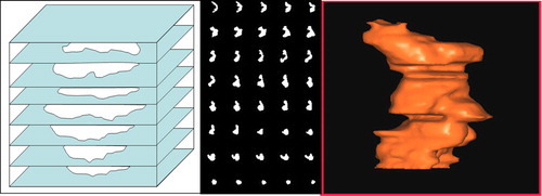
Figure 2. A demonstration of the Difference of Gaussians (DoG) identification of the edge of a homogeneous tumour is shown. As a consequence of scanning, image reconstruction and post-reconstruction filtering, the ideal intensity distribution, A, is convolved with the Gaussian point spread function to give the distribution B. A further convolution with the point spread function, carried out by computer processing, gives the distribution C. The difference B-C has its zero crossing at the edge (arrow). In this illustration, the distributions are functions of one coordinate (x) only. In the actual DoG algorithm, the distributions as well as the point spread functions are 3D entities.
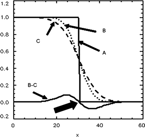
Figure 3. Illustration of the images involved in the calculation of average distance between the (correct) reference contour and the contour determined from the corresponding PET image. The tumour area (left) determined from PET is used to find the PET-derived tumour contour image (middle) that forms the basis for computation of the distance image (red parts of the right image). Each pixel in this image contains the distance to the nearest PET-derived contour. The CT-derived reference contour image (green) is superimposed on this image and distances sampled under each point of this contour. Finally, the average (rms) distance is calculated (refer to text).
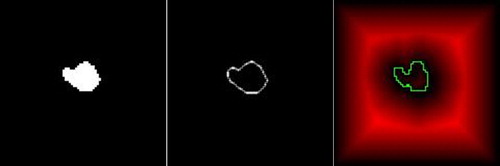
Figure 4. An illustration of the performances of different methods for tumour delineation based on PET is shown. The reference contour (red) is drawn into the PET-images, and as references for delineation based on the Difference of Gaussians (DoG) (green), manual delineation (blue) and 50% of SUVpeak isocontour delineation (black). Moving from the upper to the lower row, three consecutive slices 1 mm apart are shown. The DoG-derived contours follow the reference very closely. Manual drawing was not capable of excluding the contributions from the sources that came into focus in the lower row, and there was a tendency to exclude thin protruding parts of the tumour. IsoSUV delineation in general was imprecise and also excluded the thinner protruding parts.
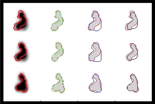
Figure 5. Illustration of the performances of different methods for tumour delineation based on PET. The reference contour (red) is drawn into the PET-images, and as references for delineation based on the Difference of Gaussians (DoG) (green), manual delineation (blue) and 50% of SUVpeak isocontour delineation (black). Moving from the upper to the lower row, four consecutive slices 1 mm apart are shown. The DoG-derived contours in row 3 are here too wide, but is correct 1 mm further up in the phantom. The isoSUV delineation here misses large parts of the protruding parts (top and second row).
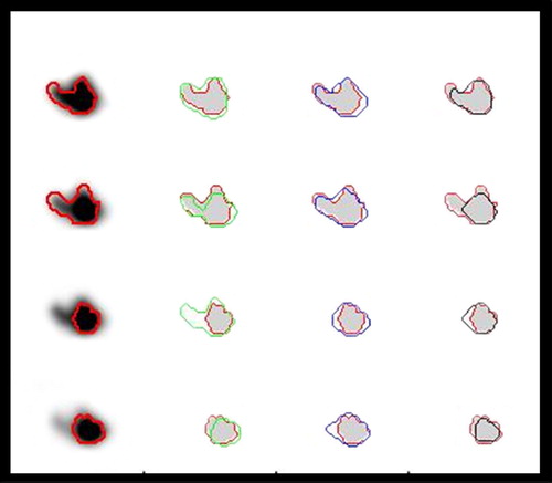
Table I. Calculated volumes and average distance deviations for different kinds of 'tumour’ delineation methods: Difference of Gaussians (DoG), manual drawing (MAN), thresholding at 50% of SUVpeak (isoSUV). ‘Expanded’ means that the calculated volume was expanded with one voxel along its entire surface. The table shows the total tumour volumes calculated and – based on the (correct) reference outlines – the percentages of tumour volume included, tumour volume missed and normal tissue volume included. The image volumes PET35 and PET50 were reconstructed with post-reconstruction Gaussian filters that had widths at half maximum (FWHM) of 3.5 and 5.0 mm, respectively. The maximum and minimum rms distance deviations were calculated for each slice individually (2D), extracting the values from the slice range from 10 to 38, and for the entire tumour surface (3D). In the 3D case voxel size was 1.33 × 1.33 × 1.0 mm, but the table lists distances calculated as if the slice distance had been 1.33 mm.