A point-selection algorithm based on spatial-stiffness analysis of rigid registration

Figures & data

Figure 1. Detail of the spatial stiffness model in the region around one of N registration points. The registration point p_i with surface normal direction n_i in its original position (gray) is displaced to new a position q_i (white) by a small rotation and translation. The spring is attached to q_i on the displaced body and to the nearest point (outlined black) on the undisplaced body.

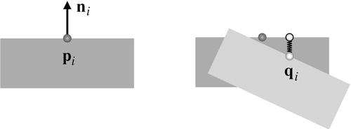
Figure 2. Two examples of the dot product d_xy. (A) A point p on a circle in the xy plane and its associated surface normal n. (B) The projection of p onto the xy plane; n is also projected but then rotated 90° in the plane. The dot product of the two vectors shown is d_xy = 0; p provides no rotational constraint about the z axis. (C) A point p on an edge in the xy plane and its associated surface normal n. (D) The projection of p onto the xy plane; n is also projected but then rotated 90° in the plane. The dot product of the two vectors shown is d_xy = ‖ p ‖; p provides good constraint about the z axis.

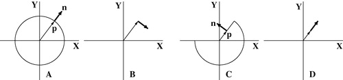
Figure 3. Computer models of the bone surfaces used in the simulations. Dark gray regions are the regions from which registration points may be selected. Targets are marked by the dark gray cubes. On the distal radius model (top left), the target is the approximate location of a screw hole for a plate used to fixate an osteotomy performed to correct a fracture malunion. On the proximal femur model (top center and right), the target is the approximate location of an osteoid osteoma. On the proximal tibia model (bottom), the target is a point on the hinge of a closing wedge osteotomy.

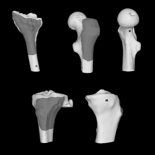
Figure 4. Distal radius surface model and registration points generated using the point-selection algorithms. From top to bottom are point sets of size 9, 18, and 30.

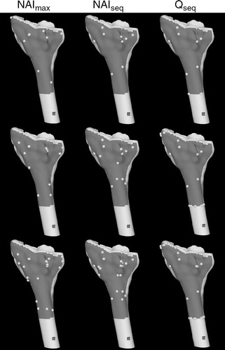
Figure 5. Proximal femur surface model and registration points generated using the point-selection algorithms. From top to bottom are point sets of size 9, 18, and 30.

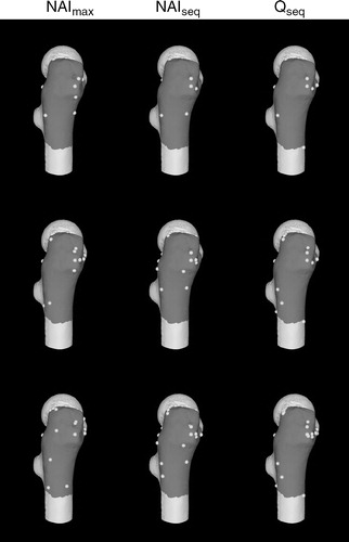
Figure 6. Proximal tibia surface model and registration points generated using the point-selection algorithms. From top to bottom are point sets of size 9, 18, and 30.

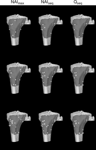
Figure 7. Registration points from Simulation set 3 generated on the distal radius by Q_seq starting from a set of six points that poorly constrain the registration problem. The six points are the almost collinear cluster on the shaft of the radius.

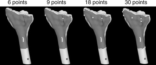
Table I.  Normalized run times of the point-selection algorithms for M = 3065. Actual run times have been divided by the amount of time required by Q_seq to generate a point set of size 9.

Algorithm	Number of registration points
	9	12	15	18	21	24	27	30
Qseq	1	2	3	4	5	6	7	8
Nseq	4	8	12	16	21	25	29	33
NAImax	180	450	800	1100	1500	2000	2600	3300

Figure 8. Results for Simulations 1 and 2 using the distal radius model. From top to bottom are average TRE, standard deviation of TRE, and maximum TRE.

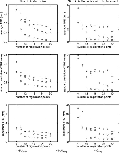
Figure 9. Results for Simulations 1 and 2 using the proximal femur model. From top to bottom are average TRE, standard deviation of TRE, and maximum TRE.

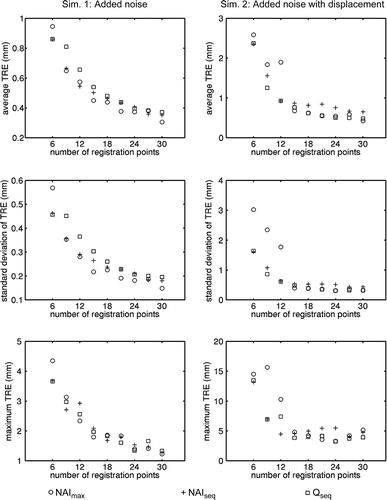
Figure 10. Results for Simulations 1 and 2 using the proximal tibia model. From top to bottom are average TRE, standard deviation of TRE, and maximum TRE.

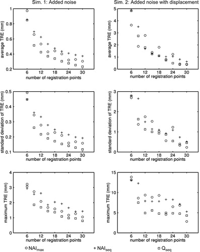
Figure 11. Results for Simulation set 3 using the distal radius model with points generated using Q_seq initialized with a set of six points that poorly constrain the registration problem. From top to bottom are average TRE, standard deviation of TRE, and maximum TRE. The solid lines are the results obtained using a good initial set of points. The results are identical to those shown in Figure 7.

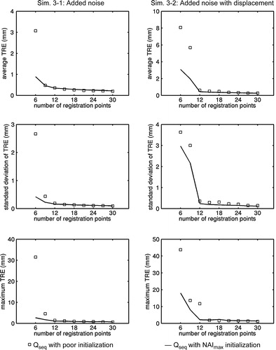
Figure 12. Results for Simulation set 4 using the proximal femur model with a version of Q_seq modified to pick the next point that contributes the least to the worst-case stiffness component. From top to bottom are average TRE, standard deviation of TRE, and maximum TRE.

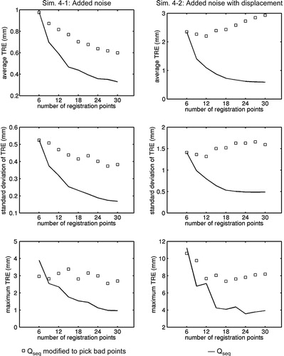
Figure 13. Results for Simulation set 5 using the proximal femur model with Q_seq and correspondence errors. From top to bottom are average TRE, standard deviation of TRE, and maximum TRE.

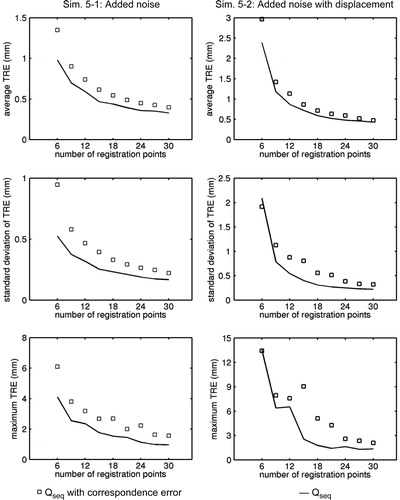
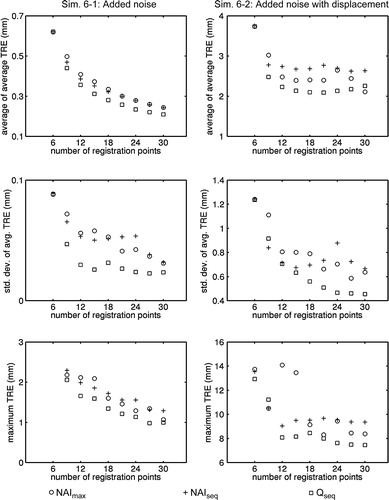
Figure 14. Results for Simulation set 6 using 10 different proximal tibial models. The top row shows the average of the 10 average TREs (), the second row shows the standard deviation of , and the third row shows the maximum TRE over all 10 models.