Predicting changes in blood flow in patient-specific operative plans for treating aortoiliac occlusive disease

Figures & data

Figure 1. Modular software architecture. Three distinct parts exist in the framework: a front-end integration environment (shown as a rectangle), an object repository (shown as a cylinder), and five modules (shown as ellipses).

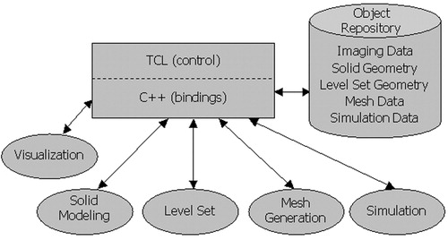
Figure 2. Overview of preoperative model construction. Initially, volumetric medical imaging data are acquired (a). Medial axis vessel paths are then extracted (b), followed by two-dimensional segmentation of the lumen boundary along each path (c). Solid models are then created for each vessel (d). Finally, the solid models representing the vessels are joined (Boolean addition) to create a solid model representing the flow domain (e). [Color version available online]

Figure 3. The software system developed in this work was used by a vascular surgeon to create virtual surgical geometric models prior to the patient's actual surgery.

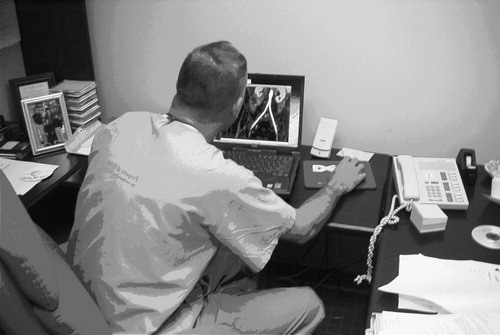
Figure 4. PCMRI slice plane acquisition locations for 67-year-old female. Seven planes of through-plane velocity information were acquired at the locations shown in the figure.

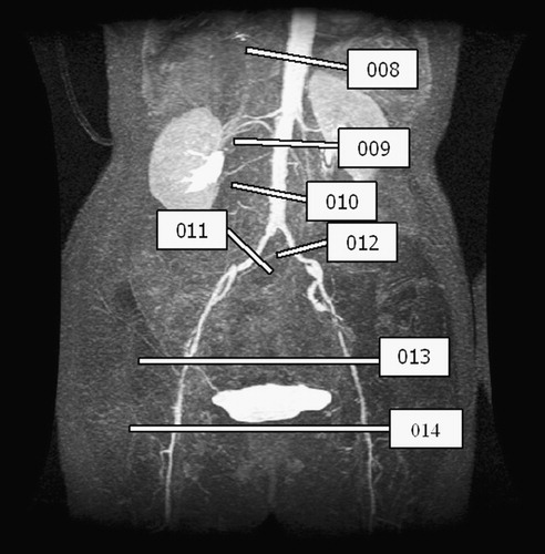
Figure 5. An example of the graphical user interface (GUI) of the system developed for surgical planning. The ‘Main Menu’ GUI guides a technician through the steps to go from medical imaging data to one- and three-dimensional hemodynamic simulation. The remaining windows in the figure are examples of controlling and running a one-dimensional analysis. [Color version available online]

Figure 6. MIP of preoperative and postoperative MRA for a 67-year-old female. (a) The extent of the occlusive disease preoperatively (notice the tight stenosis in the patient's left external iliac) and (b) the bypass graft and the occlusion of the external iliac arteries postoperatively.

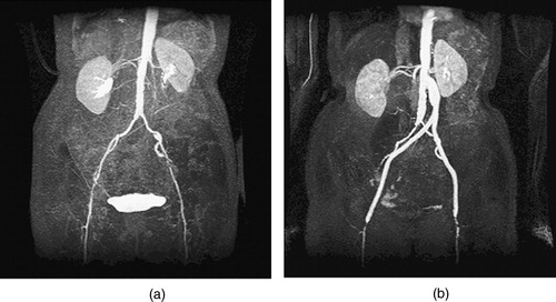
Figure 7. Two surgical alternatives for the 67-year-old female. (a) The preoperative model constructed prior to surgery. (b) A close-up of a high-grade stenosis in the left femoral artery. (c) The idealized endovascular repair (angioplasty and stenting), and (d) an aorto-femoral direct reconstruction using a Dacron bifurcating graft. [Color version available online]

Figure 8. Anatomic variability caused by vascular disease. The preoperative solid model is shown (in red) with three views created from the MRA data using thresholding. (a) The celiac trunk is not patent because of advanced vascular disease. (b) A dissection near the branch of the left internal iliac artery. (c) A tight stenosis that causes the vessel to appear disjoint because of the limitations in the image resolution and the threshold value selected. [Color version available online]

Figure 9. Two different time points of the supra-celiac aorta acquired using PCMRI. During peak systole (a), the supra-celiac aorta is approximately 20 pixels across and the lumen boundary is clearly visible in the zoomed view of the magnitude of the gradient plot (b). However, during parts of diastole, the lumen boundary is not as clearly defined, as seen in (c) and the corresponding zoomed magnitude of the gradient plot (d).

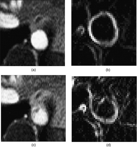
Table I.  Mean volumetric flow rate, vessel cross-sectional area, and diameter from PCMRI data.

Series*	Location	Mean volumetric flow (ml/min)	Mean area (mm^2)	Effective diameter (mm)
8	Supra-celiac aorta	2247	417.97	23.07
9	Infra-renal aorta	796	110.30	11.85
10	Supra-bifurcation	716	109.00	11.78
11	Right common iliac	320	39.30	7.07
12	Left common iliac	400	45.10	7.58
13	Right infra-internal iliac	263	29.70	6.15
13	Left infra-internal iliac	214	20.30	5.08
14	Right femoral	148	20.30	5.08
14	Left femoral	119	12.50	3.99

*Refer to Figure 4.

Table II.  Mean volumetric flow rates from postoperative PCMRI data.

Location	Mean volumetric flow rate (ml/min)
Supra-SMA	2171
Infra-renal supra-bypass	492
Right common iliac	90
Left common iliac	113
Bypass body	230

Table III.  Iterations to calculate resistance values for three-dimensional simulation to match target mean volumetric flow distribution.

Vessel	Target flow rate (ml/min)	Volumetric flow rate (ml/min)				Deviation from target mean flow rate (%)
		Sim 1	Sim 2	Sim 3	Sim 4	Sim 1	Sim 2	Sim 3	Sim 4
Supra-celiac	2247	2247	2247	2247	2247	0.0	0.0	0.0	0.0
SMA	725	662	706	717	719	−8.7	−2.7	−1.2	−0.8
Left renal	363	385	364	357	354	6.3	0.4	−1.6	−2.3
Right renal	363	339	361	366	366	−6.5	−0.6	0.8	0.9
Infra renal	796	860	816	808	807	8.0	2.6	1.5	1.4
Left common iliac	392	408	396	397	398	3.9	0.9	1.2	1.4
Right common iliac	404	451	422	413	410	11.9	4.5	2.3	1.5
Internal left iliac	182	216	190	186	185	18.4	4.1	1.9	1.6
Internal right iliac	146	170	152	149	148	16.9	4.2	2.0	1.4
Left femoral	210	192	206	211	212	−8.7	−1.8	0.5	1.2
Right femoral	258	281	270	264	262	9.0	4.6	2.5	1.5

Sim = simulation.

Figure 10. Rest and exercise supra-celiac flow waveforms for the 67-year-old female. The rest flow waveform was experimentally acquired using PCMRI. The exercise flow waveform was generated by shortening the diastolic portion of the rest curve by one-third and scaling the mean volumetric flow rate by a factor of two.

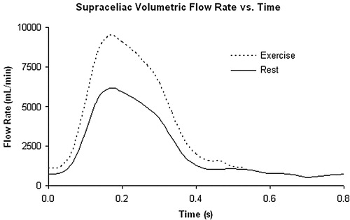
Figure 11. Exterior surface mesh for the model of the 67-year-old female patient. The mesh consists of 1.8 million tetrahedral elements.

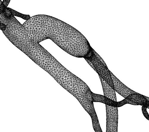
Figure 12. Mean wall shear stress for preoperative model. (a) shows the mean wall shear stress for the entire preoperative model. (b) shows a zoomed anterior view of the infra-renal aorta, while (c) shows a posterior view of the infra-renal aorta. Notice the region of low mean wall shear stress located just proximal to the aortic bifurcation, an area predisposed to atherosclerosis.

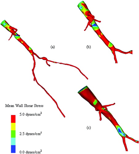
Figure 13. Mean wall shear stress for AFB model. Regions of low mean wall shear stress (shown in blue) are theorized to be sites of high risk for the development of atherosclerosis or neointimal hyperplasia.

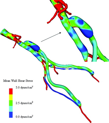
Figure 14. Scalar clearance time for AFB model. (a) The scalar field is initially set to 1.0 (shown in red) with a zero scalar Dirichlet boundary condition at the inlet. The scalar is then advected and diffused out of the flow domain over several cardiac cycles (where time is increasing from (a) until the final time point shown in (d)). The vessel walls have a scalar flux of zero.

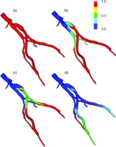
Table IV.  Comparison of mean volumetric flow rates from three-dimensional simulations of rest and exercise.

Location	Rest			Exercise
	Preoperative (ml/min)	AFB (ml/min)	Stent (ml/min)	Preoperative (ml/min)	AFB (ml/min)	Stent (ml/min)
IR aorta (proximal bypass)	792	888	837	3472	3901	3660
Bypass body		555			2340
IR aorta (distal bypass)		333			1564
Bypass right limb		247			1098
Bypass left limb		306			1243
Right external iliac	258	14	248	1107	73	1053
Left external iliac	208	2	276	527	− 23	907
Right femoral	258	262	248	1107	1171	1053
Left femoral	208	309	276	527	1221	907

Table V.  Zero frequency mode of impedance boundary conditions at outlets for rest and exercise.

Vessel outlet	Root radius (cm)	Length- to-radius ratio	Z(0) rest (dyne*s/cm^5)	Z(0) exercise (dyne*s/cm^5)
Right femoral	0.202	40.34	36277	6197
Left femoral	0.203	34.37	30460	5739
SMA	0.192	10.07	10365	33049
Left renal	0.157	15.35	26393	85335
Right renal	0.154	11.59	21027	68957
Left internal iliac	0.257	115.28	55029	11726
Right internal iliac	0.159	41.49	68649	10550

Table VI.  Mean volumetric flow results from one-dimensional simulations.

Location	Rest			Exercise
	Preoperative (ml/min)	AFB (ml/min)	Stent (ml/min)	Preoperative (ml/min)	AFB (ml/min)	Stent (ml/min)
IR aorta (proximal bypass)	726	777	762	3843	4057	3947
Bypass body		479			2193
IR aorta (distal bypass)		299			1864
Bypass right limb		213			1012
Bypass left limb		268			1182
Right external iliac	232	18	226	1353	235	1166
Left external iliac	212	7	261	484	135	1106
Right femoral	232	232	226	1353	1247	1166
Left femoral	212	276	261	484	1318	1106

Table VII.  Pressure results from one-dimensional simulations.

Location	Preoperative rest			Preoperative exercise
	Mean (mmHg)	Max (mmHg)	Min (mmHg)	Mean (mmHg)	Max (mmHg)	Min (mmHg)
IR aorta (proximal bypass)	111.0	148.4	78.1	160.8	203.6	111.2
Bypass body
IR aorta (distal bypass)
Bypass right limb
Bypass left limb
Right external iliac	107.3	148.0	74.1	115.0	142.8	81.4
Left external iliac	83.1	102.1	63.0	41.1	47.1	32.8
Right femoral	105.6	147.5	72.5	105.3	132.2	73.1
Left femoral	81.1	100.3	61.1	35.7	40.8	28.5
	AFB rest			AFB exercise
IR aorta (proximal bypass)	106.9	129.0	85.7	112.6	138.6	83.5
Bypass body	107.1	130.0	85.1	114.0	141.2	82.7
IR aorta (distal bypass)	107.0	129.7	85.2	112.9	139.6	82.7
Bypass right limb	107.0	131.4	83.8	113.1	142.4	80.1
Bypass left limb	106.9	130.6	84.1	112.9	141.6	80.5
Right external iliac	106.5	130.6	83.6	105.4	131.6	75.8
Left external iliac	105.8	129.3	83.1	96.6	119.5	70.3
Right femoral	105.7	130.2	82.4	97.3	121.7	69.8
Left femoral	105.4	128.9	82.6	95.2	118.2	69.0
	Stent rest			Stent exercise
IR aorta (proximal bypass)	108.2	144.8	76.0	138.6	185.3	85.8
Bypass body
IR aorta (distal bypass)
Bypass right Limb
Bypass left limb
Right external iliac	105.0	144.3	72.6	101.4	133.7	63.7
Left external iliac	102.2	136.3	71.4	92.4	116.8	62.0
Right femoral	103.0	143.9	70.5	91.1	120.1	57.1
Left femoral	100.0	134.1	69.4	80.3	101.3	54.0

Table VIII.  Mean volumetric flow-rate differences between three-dimensional and one-dimensional simulations.

Location	Differences for rest simulation			Differences for exercise simulation
	Preoperative (%)	AFB (%)	Stent (%)	Preoperative (%)	AFB (%)	Stent (%)
IR aorta (proximal bypass)	− 8.1	− 12.5	− 9.0	10.7	4.0	7.8
Bypass body		− 13.7			− 6.3
IR aorta (distal bypass)		− 10.3			19.2
Bypass right limb		− 13.8			− 7.8
Bypass left limb		− 12.5			− 4.9
Right external iliac	− 10.0	32.0	− 9.1	22.2	222.6	10.7
Left external iliac	2.5	260.0	− 5.5	− 8.3	− 693.8	21.9
Right femoral	− 10.0	− 11.5	− 9.0	22.2	6.5	10.7
Left femoral	2.5	− 10.8	− 5.4	− 8.3	8.0	22.0

Figure 15. MIP of preoperative and postoperative MRA for a 55-year-old male. (a) shows the extent of the occlusive disease preoperatively (the tight stenosis in the left and right external iliac arteries), while (b) shows the bypass graft. Postoperatively, the distal native aorta and the external iliac arteries are occluded. The postoperative data were acquired 9 days after the surgery.

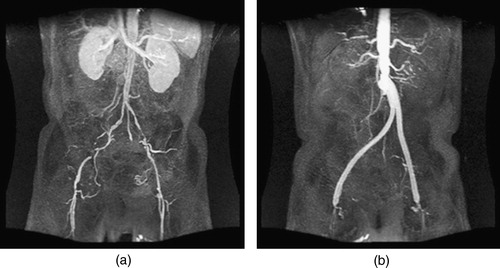
Figure 16. Views of the proximal anastomosis from the postoperative MRA dataset for the 55-year-old male. An isosurface of the postoperative MRA data set in the neighborhood of the proximal anastomosis is shown from two different angles. The distal native aorta occluded after surgery. [Color version available online]

Figure 17. Two bypass plans for 55-year-old male patient. (a) shows the preoperative model, (b) shows plan 1, and (c) shows plan 2. In (d), both plans are shown together to highlight differences between the two plans. [Color version available online]

Figure 18. Mean wall shear stress for plan 1. (a) the entire model; (b) an anterior view; and (c) a posterior view of the proximal anastomosis.

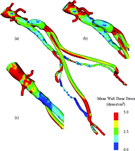
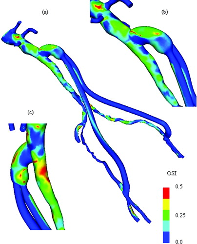
Figure 19. OSI for plan 1. (a) the entire model; (b) an anterior view; and (c) a posterior view of the proximal anastomosis.