Theoretical model for laser ablation outcome predictions in brain: calibration and validation on clinical MR thermometry images

Abstract

Purpose: Neurosurgical laser ablation is experiencing a renaissance. Computational tools for ablation planning aim to further improve the intervention. Here, global optimisation and inverse problems are demonstrated to train a model that predicts maximum laser ablation extent.

Methods: A closed-form steady state model is trained on and then subsequently compared to N = 20 retrospective clinical MR thermometry datasets. Dice similarity coefficient (DSC) is calculated to provide a measure of region overlap between the 57 °C isotherms of the thermometry data and the model-predicted ablation regions; 57 °C is a tissue death surrogate at thermal steady state. A global optimisation scheme samples the dominant model parameter sensitivities, blood perfusion (ω) and optical parameter (μ_eff) values, throughout a parameter space totalling 11 440 value-pairs. This represents a lookup table of μ_eff–ω pairs with the corresponding DSC value for each patient dataset. The μ_eff–ω pair with the maximum DSC calibrates the model parameters, maximising predictive value for each patient. Finally, leave-one-out cross-validation with global optimisation information trains the model on the entire clinical dataset, and compares against the model naïvely using literature values for ω and μ_eff.

Results: When using naïve literature values, the model’s mean DSC is 0.67 whereas the calibrated model produces 0.82 during cross-validation, an improvement of 0.15 in overlap with the patient data. The 95% confidence interval of the mean difference is 0.083–0.23 (p < 0.001).

Conclusions: During cross-validation, the calibrated model is superior to the naïve model as measured by DSC, with +22% mean prediction accuracy. Calibration empowers a relatively simple model to become more predictive.

Keywords:

• Neoplasm metastasis
• laser tissue ablation
• neurosurgery

Introduction

Some of the most debilitating maladies – primary neoplasms, secondary neoplasms, radiation necrosis and epilepsy – manifest in the brain and may require neurosurgical management. Magnetic resonance (MR)-guided laser induced thermal therapy presents an opportunity to improve surgical care in these patients via an image-guided, repeatable, well-tolerated procedure [1–4]. Between primary and secondary brain tumours, metastases represent the larger burden to human welfare with an order of magnitude greater incidence as gliomas while sharing a similarly dire prognosis [5–7]. The value in studying secondary brain cancer is increasing, especially as brain metastasis patients live longer via better extracranial disease management [8]. A common treatment for brain neoplasms is radiotherapy, with stereotactic radiosurgery being a chief tool [7,9–11]; however, a small but considerable fraction of treated patients develop radiation necrosis and may require neurosurgery [12–15]. MR-guided laser ablation has been investigated for these patients [16–19]. Interest is burgeoning for MR-guided laser ablation as the means of intervention in paediatric epilepsy surgery [20–28] with some analysis studying the efficacy/complication thresholds at which MR-guided laser ablation is a superior intervention [29]. In summary, laser ablation is being investigated as an alternative to traditional resections for malignancy, radiation necrosis and paediatric epilepsy.

While MR-guided laser ablation has powerful real-time guidance [30–33], the procedure stands to improve via pre-surgical a priori planning. If there were means to reliably predict the outcome of a laser ablation – e.g. the ablated region for a given location and power history – then neurosurgeons would be able to implement inverse treatment planning. Inverse treatment planning is commonly used in radiotherapy [34,35] and has been conceived for use in interstitial thermal therapy [36–38]. This would allow clinicians to #1. Identify where to best place the laser applicator and #2. Decide when multiple applicators would be advantageous. This planning information would behove all MR-guided laser ablations; however, it would especially benefit clinics that do not have access to an intraoperative MR suite. Without intraoperative MR, anaesthetised patients are moved mid-procedure from the surgical suite to the MR suite [20,22,24,27]. Effective planning in these clinics further minimises the chance that the procedure requires repeating, that the patient will be iteratively moved between the MR suite and the surgical suite in order to best place the applicator, and/or the procedure be abandoned mid-procedure.

The Pennes bioheat transfer equation [39] is a partial differential equation that has been extensively used to describe heat transport in biological systems and laser ablation in particular. When paired with a damage model [40–45], the bioheat transfer equation can be used to predict various thermal effects; here, tissue kill is most interesting. A chief source of model inaccuracy is the dearth of model constitutive values from patient-specific, disease-specific or otherwise salient measurements [46–48]. Traditionally, gradient-based optimisation [38,48,49] is implemented for calibration of the bioheat transfer equation to the available thermal imaging data. In the context of biothermal simulation, global optimisation is typically avoided because of the computational expense associated with the simulation methods [37,38,49]. This manuscript demonstrates that a global optimisation strategy is feasible for MR-guided laser induced laser ablation treatment planning. Global optimisation is enabled by efficient graphical processing unit (GPU) kernels for an exhaustive search of the parameter space needed for model calibration. Hash function lookups, i.e. lookup tables, are used for cross-validation [50–54] of prediction accuracy. The resulting model predicts the maximum ablation extent for the purpose of surgical planning.

Methods

In this work, an inverse problem is used to calibrate a model’s parameters – also called “model training” or “model calibration”. First, the components of the inverse problem are expounded. After model calibration, a simulated validation is executed using leave-one-out cross-validation. The Methods and the Supplemental are significantly based on a Ph.D. dissertation chapter, which was made available in December 2016 [55].

Components of model calibration

Broadly speaking, an inverse problem brings a simulation into agreement with physical reality by varying the simulation’s input parameters. Agreement is measured via an objective function. The implemented inverse problem requires four components: (1) a gold standard measurement of the physical system, (2) a model to predict that physical measurement, (3) an objective function that measures goodness of fit between the gold standard measurement and the model and (4) an optimisation algorithm that minimises the objective function. These four components are illustrated in Figures 1 and 2 and described in the following Methods sections. Again, the purpose of the model is to predict the maximum ablation extent.

Figure 1. Subfigure (A) is the model’s temperature prediction that optimises the objective function, Dice similarity coefficient (DSC). Subfigure (A) is juxtaposed with a time frame from clinical MR thermometry that is near steady state, Subfigure (B). Subfigure (C) is the 57 °C isotherm map, showing where the thermometry and model overlap or do not. The threshold map of subfigure (C) is used to compute DSC. For this image, DSC is 0.88. Subfigure (D) displays the global optimisation of the model to this particular patient’s thermal dataset, seeking to optimise DSC. The vertical axis is the values of perfusion, ω, and the horizontal axis is the values of the effective optical coefficient, μ_eff. The single point that produces optimal DSC is the dot in subfigure (D), or μ_eff=166 m⁻¹ and ω = 9.5 kg m⁻³ s⁻¹.

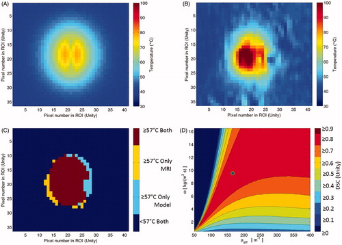
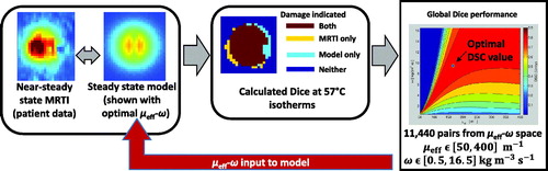
Figure 2. This diagram illustrates the four major components of the global optimisation, using the four images of Figures 1. The gold standard measurement is the MR thermometry from a time point near steady state. This thermal image is compared to the steady state kernel via DSC of the 57 °C isotherms. The kernel is run with 11 400 μ_eff–ω values; each model realisation reports a DSC value and is recorded in the optimisation map at right.

Gold standard measurement: 57 °C isotherms from MR thermometry cohort

A gold standard measurement of physical reality provides a goal for the simulation to fit. There are N = 20 MR thermometry series with 5 s time frames from MR-guided laser induced thermal therapy procedures using the water-cooled Visualase (Medtronic, Inc., Minneapolis, MN) 980 nm laser surgical device. It, which has a maximum power setting of 15 W. The thermometry data have two spatial dimensions, i.e. it is single-slice. The 20 individual ablations use laser powers ranging between 9.75 W and 12.9 W with a median and mode of 12 W. Patient recruitment and treatment included informed consent, consistent with an institutional review board. The MR was a 1.5 T MRI (GE Healthcare Technologies, Waukesha, WI). The thermometry was a 2D gradient echo sequence (flip angle = 30°, field of view = 24 * 24 cm², matrix size = 256 * 128, repetition time/echo time = 37.5/20 ms, receive-only head coil, 5 s per time frame) [56].

The main effect of interest during the ablation is the extent of lethal tissue damage. Thermal damage can be indicated by Arrhenius damage, cumulative effective minutes, or a lethal threshold temperature in the case of fast and high heating [40–45]. Here, the gold standard physical measurement is the 57 °C isotherm, which represents the tissue that is irreversibly damaged. Given the fundamental time-integrated nature of thermal dose [42,45,57], the use of the 57 °C isotherm demands explanation. The implemented steady state model presents challenges for integrating time in order to determine the extent of irreversible damage, as is the case for Arrhenius and CEM thermal dosimetry models. A method to estimate the extent of damage using a steady state computational model is to assume the physician controlling the therapy has the option to hold the ablation at near-steady state for two MR thermometry frames. By holding the temperature of a thermal image voxel at 57 °C for two MR thermometry frames (i.e. 10 s), there is a high confidence that the tissue will suffer irreversible damage. The Supplemental demonstrates that tissue at 57 °C accrues a thermal dose of Ω = 1 at ∼7.4 s using Henriques’ parameters.

Analytic steady state computational model of heating

The second component of the inverse problem is a model kernel for the prediction of the heating as measured by the gold standard measurement, i.e. MR thermometry. Here, it is an analytic steady state kernel expressed in Equations (4)–(6) of the Supplementary materials [48,55,58–61]. The use of the steady state kernel here is motivated by the relatively close performance of a trained steady state kernel with a more sophisticated trained transient finite element model in Fahrenholtz et al. [48].

The steady state kernel uses two patient-specific inputs to model a particular patient’s ablation. Firstly, the patient’s laser power from the first ablative heating is recorded. Secondly, the laser fibre’s in-plane angle is used to register the model and actual ablations in matching regions of interest (ROI). Additionally, the following two laser-bioheat parameters are variable inputs: an effective optical coefficient, μ_eff, and a blood perfusion rate, ω. The choice to optimise the μ_eff and ω parameters is motivated by a previous investigation that identified model-parameter sensitivities [47]. Finally, the kernel output is a 2D temperature field (i.e. a single slice) at steady state with 57 °C representing the maximum extent of ablation for the given power and location.

The use of an isotherm as a proxy for thermal dose requires a handful of assumptions in order to ensure predicted ablation sizes are safely conservative (i.e. small ablations that are confidently possible). The purpose of conservativism is to prevent the surgical situation where more laser applicators are deemed necessary mid-intervention because of inadequately small ablations. The first assumption is that the laser-on time duration must be short (about 150 s or less), which reduces the potential for thermal dose to accrue from lower temperatures (43–53 °C) through time. Secondly, the target tissue cannot have been previously heated substantially. Thirdly, the ablation must approach steady state. This third assumption is motivated by the computational model’s steady state assumption and is only necessary for training the model; model training is described later within the Methods section concerning optimisation. Some patient MR thermometry series include multiple heating pulses. Among the N = 20 MR thermometry series, only the first ablative heating (i.e. ignoring test pulses) sufficiently conform to these assumptions to compare with the computational model. Among the time frames imaging the first ablative heating, the last laser-on time frame is used to compare against the computational model. It is possible that the first two assumptions could be relaxed and the steady state model may still have utility, but that is beyond the scope of this investigation.

Two key features that enable the kernel’s success and ability to be optimised globally are GPU-acceleration and the kernel’s temperature linearity with laser power. The kernel’s temperature linearity property allows the simulation of arbitrary laser powers by using linear combinations of simulations using laser powers of 0 W (P = 0 W) and P = 1 W. The P = 0 W case is included to model the water-cooling effect, and the P = 1 W case is to model the heating in the presence of cooling as well. Consequently, for a given pair of optical and blood perfusion values, the steady state kernel’s P = 0 W and P = 1 W simulations are used to recreate patient-specific power settings without uniquely calculating the patient-specific power. The model’s temperature linearity with laser power is demonstrated in the Supplemental, especially Supplemental Figure 1. Meanwhile, the GPU-acceleration massively parallelises the P = 0 W and P = 1 W simulations, expediting their calculation.

Objective function: Dice similarity coefficient (DSC)

As a well-designed objective function is minimised, it brings the model into agreement with the gold standard measurement. In this manuscript, the primary objective function is the DSC [62] and has found general use for comparing regions [63] and, in particular, tissue regions purported to have suffered lethal thermal damage [44,48,64,65]. DSC is a metric that quantifies the overlap between two regions and is defined as two times the intersection of two regions, normalised by the summed areas of the two regions.

A is the region exceeding 57 °C near steady state from patient MR thermometry data. B is the region enclosed by the 57 °C isotherm contour for the model while using the patient-specific laser power and in-plane laser fibre angle. DSC ranges from 0 (no overlap) to 1 (exact overlap). DSC ≥0.7 is considered a threshold at which the agreement of the regions suggests the model is useful [44,63,66]. The patient data only include examples with fast heating that approach steady state. In order to investigate the objective function’s sensitivity to threshold temperature, isotherm thresholds ranging from 51 to 65 °C are tracked (all 15 integer temperature values). The Supplemental presents the Arrhenius thermal dose for a range of candidate temperatures; the Arrhenius thermal dose model, with Henriques’ parameters [67], is used by the Visualase system for real-time dose estimation [68].

Constrained global parameter optimisation in effective optical coefficient and blood perfusion parameter space (μ_eff–ω space)

The simplifying approximations of the steady state kernel expedite its computation. The result is the steady state kernel can be optimised, i.e. “trained,” using a global parameter search. The search domain is a two-dimensional parameter space that includes the effective optical coefficient (μ_eff) and blood perfusion (ω) parameters. This μ_eff–ω space is densely sampled by a regular grid search scheme, which constitutes the global optimisation.

In order to optimise a single patient dataset, each μ_eff–ω pair is submitted to the steady state model which creates a steady state temperature prediction. To create isotherm regions, the many temperature predictions are thresholded at the integer temperature values ranging from 51 to 65 °C with 57 °C being the threshold of chief interest. The patient thermometry from near-steady state is also thresholded at the same temperatures to create isotherm regions. Next, DSC is calculated for each μ_eff–ω pair at each isotherm temperature, which compares the patient thermometry to the model. For a given isotherm temperature and patient, the μ_eff–ω pair that produces the maximum DSC value represents the optimal parameter pair.

In the regular grid search, the blood microperfusion space is constrained to ω∈[0.5,16.5] kg m^-3 s^-1 with 65 evenly spaced samples; it encompasses the plausible physical range of ω values and beyond. The effective optical coefficient space is constrained to μ_eff∈[50 400] m^-1 with 176 evenly spaced samples. The μ_eff range covers the range useful to the model, but is not physical. At very low μ_eff values, the model produces spatially small ablations. At high end of the μ_eff range, the model produces its maximum spatial extent of ablation. μ_eff values higher than the range progressively shrink the ablation size. The total number of μ_eff–ω pairs is multiplicative; 65 ω samples * 176 μ_eff samples is 11 440 total μ_eff–ω pairs. For the regular grid search, there are 11 440 simulations with a power setting of 1 W (P = 1 W). However, there are only 65 P = 0 W simulations since varying μ_eff – i.e. the optical parameter – does not change a P = 0 W simulation. Ergo, a total of 11 505 simulations is necessary to sample the entire μ_eff–ω space for P = 0 W and 1 W. Since the optimisation algorithm in this manuscript is global, all 15 isotherms (51–65 °C) are able to be tracked and optimised on the same set of 11 505 simulations. Using these same simulations, the 15 different isotherm contours are applied to the model and MR thermometry, then compared via DSC and recorded. The 1 W and 0 W temperature maps for each point in μ_eff–ω parameter space are generated by the steady state kernel and saved as lookup tables; the kernel is then no longer used. By taking advantage of the model’s linearity with laser power, the 1 W and 0 W temperature maps can match an arbitrary single slice MR thermometry dataset by adjusting the power and in-plane laser fibre angle of orientation. The technique avoids the need to run the computational kernel for each individual dataset; instead, it runs through every μ_eff–ω pairing once for all datasets.

Leave-one-out cross-validation via vector map manipulation

The previously described inverse problem was for the purpose of identifying the optimal μ_eff–ω pair for each patient dataset. However, mere optimisation of μ_eff–ω for the individual patients does not provide information on the trained model’s predictive accuracy. Leave-one-out cross-validation is used to simulate the N + 1 prediction case. Given the global nature of the optimisation algorithm, the computational cost required to identify the μ_eff–ω pair that optimises the average objective function, DSC, among all patients is negligible; access to the global behaviour of DSC in μ_eff–ω space provides powerful information.

Before cross-validation begins, the μ_eff–ω global optimisation using regular grid sampling is executed. The result of optimisation of an individual patient’s thermometry dataset is a 2D map in μ_eff–ω space of the DSC performance. These 2D maps of individual optimisations are superimposed to create a vector map of DSC performance among the patient datasets. It can be conceived as a lookup table or a 3D dataset – one dimension of μ_eff, one dimension of ω, and one dimension of DSC performance among the datasets in the patient cohort. The size of the vector map is where V_size the total number of elements in the vector map, N_μeff is the number of μ_eff samples, N_ω is the number of ω samples and N is the number patients in the cohort. Here, N_μeff=176 and N_ω=65 and N = 20. In total, there are 228 800 elements of DSC response for one isotherm. The entire cross-validation algorithm thereafter is only manipulations of a lookup table, i.e. the vector map.

A variety of manipulations can be applied to interrogate the vector map; e.g. the mean, median, and standard deviation of the vector map’s DSC dimension respectively yield 2D maps of the DSC’s mean, median, and standard deviation. A heuristic demonstration of the vector map’s construction is found in Figure 3. Here, the vector map can be queried using descriptive statistics or thresholds, e.g. the DSC ≥ 0.7 limit which demarcates success/failure when using DSC.

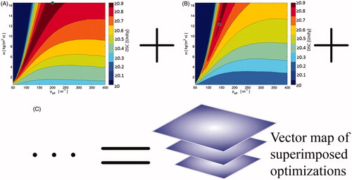
Figure 3. This is a cartoon demonstration of the superposition of individual datasets’ global optimisation in μ_eff–ω space. Each dataset’s optimisation performance, e.g. (A) and (B), can be superimposed pixel-wise in μ_eff–ω space to create an optimisation vector map (C). This optimisation vector map has N = 20 individual optimisation results for every sampled point in μ_eff–ω space. At every point in the optimisation vector map, descriptive statistics can describe the distribution’s behaviour at that μ_eff–ω point, see Figure 4.

During one iteration of leave-one-out cross-validation of N number of patients, a vector map is constructed using the N− 1 individual optimisation maps. Then, a mean operator is applied to the 3D vector map, resulting in a 2D mean DSC map. In this N− 1 DSC mean map, the μ_eff–ω pairing that produces the greatest average DSC value is subsequently used to predict the left-out patient dataset; the predictive DSC performance is recorded. This concludes one iteration of leave-one-out cross-validation. The remainder of the cross-validation algorithm is to permute the left-out dataset until all datasets have been left out once. Exhaustive permutation of the cross-validation algorithm requires N iterations.

Statistical comparison

A pertinent statistical question is whether or not there is a difference of DSC performance for the model using naïve literature values and the optimised model during leave-one-out cross-validation. This can be addressed via a paired Student’s t-test to compare the means of the two methods’ DSC performances; the null hypothesis is that the means of the model using naïve literature values and the optimised model during cross-validation are the same. A p value and a 95% confidence interval of the difference of means are reported. The statistical comparisons are executed by GraphPad Prism 6 (GraphPad Software, La Jolla, CA).

Results

Optimisation

The optimisation performance of DSC is best summarised in the “SS DSC opt.” column of Table 1. The optimal mean DSC performance is 0.8889 with all 20 patient datasets passing DSC ≥0.7 during optimisation, compared to the naïve literature value model’s 0.6685. Figure 4’s subfigures display the DSC vector map when different statistical and threshold operators are applied. In Figure 5, the points in μ_eff–ω space that create optimal DSC values are shown. In order to measure the model’s sensitivity to isotherm threshold choice, a box-and-whisker plot displaying the distribution of optimal DSC values with increasing isotherm threshold temperature is shown in Figure 6.

Figure 4. These are the descriptive statistic maps based on the vector map, described in Figure 3. The diamond icons mark the naive literature value choice, μ_eff=180 m^–1 and ω = 6 kg m^–3 s^–1. (A) is the mean; (B) is the median; (C) is the standard deviation; (D) is the number of individual patient datasets that pass DSC ≥0.7.

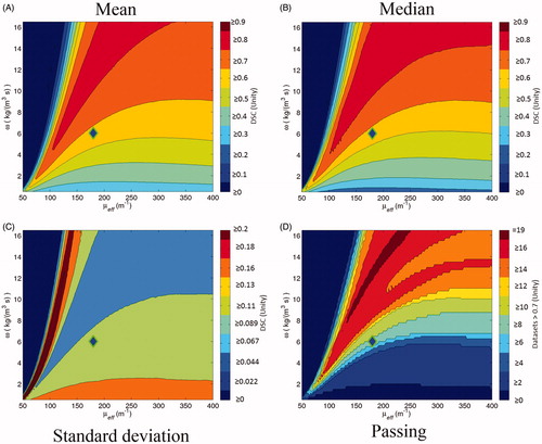
Figure 5. This scatter plot indicates the points in μ_eff–ω space that create optimal DSC values for individual datasets among the N = 20 datasets. There is a simple linear regression fit line (in blue) of the 18 optimal points (markers are blue with green outlines) that define the line. The fit line’s details are listed in the Results. There are two clearly outlying optimal points, isolated to the figure's right side. These points are excluded from the fit line, but are included in leave-one-out cross-validation. The scatter plot and fit line are superimposed over the mean of the DSC vector map; i.e. Figure 4(A).

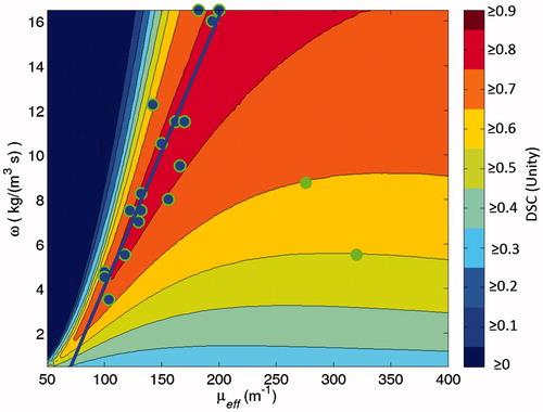
Figure 6. This is a box-and-whisker plot demonstrating the model’s sensitivity to isotherm choice during optimisation; each row represents the distribution of N = 20 patient cohort’s DSC performance during optimisation while using a particular isotherm temperature. 57 °C is the choice implemented in the rest of the work. In the box-and-whisker plot, the solid dots are the minima and maxima, i.e. the ends of the whiskers. The box is the 95% confidence interval and the line within the box is the median. A single dataset among the cohort is not robust with varied isotherm threshold. It is the leftmost outlier and performs worse with rising isotherm threshold, especially at 58 °C and higher. The other datasets do not vary much with isotherm choice.

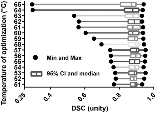
Table 1. Here are the descriptive statistics for DSC performance by using naïve literature values, optimised parameters, and during leave-one-out cross-validation using the vector map method for N = 20 datasets.

Descriptive statistic	Dice Naïve (Unity)	Dice opt. (Unity)	Dice LOOCV (Unity)
Minimum	0.45	0.75	0.59
25%-ile	0.61	0.87	0.77
Median	0.66	0.90	0.85
75%-ile	0.77	0.91	0.88
Maximum	0.86	0.95	0.93
DSC ≥0.7	8	20	19
Mean	0.67	0.89	0.82
Standard deviation	0.11	0.047	0.089
Skewness	−0.23	−1.3	−1.0
Kurtosis	2.3	5.4	3.6

The optimal column represents the best possible DSC performance that the steady state model can achieve within the μ_eff–ω parameter space explored. Note that all DSC, skewness, and kurtosis quantities are unitless. “%-ile” refers to percentiles; e.g. 25%-ile means the dataset’s DSC performance exceeds 25% of the population DSC values in ascending ranked order. DSC: Dice similarity coefficient; naïve: naïve literature values were used in model; opt.: optimal Dice similarity coefficient possible for model; LOOCV: model performance during leave-one-out cross-validation.

In Figure 5, there is a blue fit line for the 18 datasets whose optimal μ_eff–ω points cluster nearby. The line is a simple linear regression calculating the optimal ω based on the optimal μ_eff. The line’s fit to the 18 points is significant (p < 0.001; R²=0.8789). The fit line equation is where a=–8.8087 kg m⁻³ s⁻¹ and b = 0.1214 kg m⁻² s⁻¹.

Among Figures 5 and 6 which display DSC performance during optimisation, three individual patients’ datasets can be identified as outliers. Two outliers are the green points in Figure 5 and one is the leftmost point in each of the box-and-whisker plots in Figure 6. These outliers are identified for illustrative purposes but not otherwise excluded since no a priori data selection criteria were able to identify them. As the isotherm threshold temperature increases, Figure 6 has a single dataset that performs extremely poorly compared to the other 19 datasets, especially at 58 °C and hotter. For optimal DSC performance using 57 °C isotherms, Figure 6’s outlier’s optimal parameter point is at μ_eff=130.0 m^-1 and ω=7.0 kg m^-3 s^-1, near the fit line of Figure 5. Two more outliers are easily identified by their distance from Figure 5’s fit line.

Leave-one-out cross-validation performance

Using the vector map method for parameter selection described earlier, the resulting leave-one-out cross-validation performance for DSC is detailed in Figure 7 and Tables 1 and 2. During cross-validation, the steady state kernel performs definitively better after training as opposed to using naïve literature values. In cross-validation, the trained model has a DSC mean = 0.82 and 19 of 20 pass DSC ≥0.7. The model naïvely using literature values has a DSC mean = 0.67 and 8 of 20 pass DSC ≥0.7. The three outlier datasets, identified during training, represent the three of the four worst performing datasets during leave-one-out cross-validation via vector map method. The remaining 16 datasets exceeded an even higher standard of at least DSC ≥0.75.

Figure 7. For the entire N = 20 cohort, this Figure displays the simulated predictive performance of the globally optimised model during leave-one-out cross-validation (solid line) versus a naïve literature value parameter choice (dashed line). A greater the area-under-the-curve, which is synonymous with the mean performance, indicates better performance.

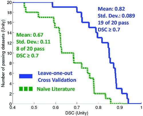
Table 2. These percentiles correspond to several interesting DSC thresholds using the N = 20 datasets.

DSC threshold (Unity)	DSC Naïve (%-ile)	DSC opt. (%-ile)	DSC LOOCV (%-ile)
0.5	11	0	0
0.6	23	0	3.1
0.7	59	0	7.5
0.8	89	5.9	34
0.85	96	13	49
0.9	100	51	86
0.95	100	95	100
0.975	100	100	100

The columns refer to the same datasets described in Table 1. The smaller the percentile value, the better the model’s performance. "0" indicates all values pass at the given threshold; “100” indicates no values pass. DSC: Dice similarity coefficient; naïve: naïve literature values were used in model; opt.: optimal Dice similarity coefficient possible for model; LOOCV: model performance during leave-one-out cross-validation.

Statistical comparison

Student’s t-test demonstrates a significant difference (p < 0.001), rejecting the null hypothesis in favour of the hypothesis that the means are different. The 95% confidence interval of the difference of DSC means ranges from 0.083 to 0.23, favouring the vector map leave-one-out cross-validation method.

Discussion

The purpose of the computational model is to predict the maximum extent of the ablation for the purpose of surgical planning. In context of planning MR-guided laser ablation, knowledge of the maximum ablation size allows the physician to decide whether a single laser fibre is sufficient. Such information can reduce cases where more laser applicators are deemed necessary mid-procedure, benefiting the intervention. In cases where the target lesion is smaller than the model-predicted maximum ablation size, the real-time MR thermometry ensures a safe and effective ablation.

It is possible that two of the three model assumptions can be relaxed while still allowing the model to make useful steady state temperature predictions; the assumptions being temporally short heating and the limitation of only considering previously unheated tissue. For this feasibility investigation, the model assumptions provide confidence that a given laser ablation’s maximum extent will not fall inside the predicted maximum extent, a situation that the model is specifically designed to prevent. Situations that would test the model assumptions of fast heating and prior heating include repeated ablations and “pull-backs”, the clinically common practice of retracting the laser fibre within the original insertion tract and ablating again. The third assumption requiring the patient’s ablation reach near-steady state is only necessary during the model’s training, i.e. patient data can be retrospectively reviewed to find ablations that near steady state temperature. A subsequent clinical ablation, hypothetically planned with the proposed model, could safely and effectively cease sooner than steady state.

Global optimisation does provide advantages in terms of the sequence of computational tasks and flexibility in objective function choice. Regarding computational advantages, the generation of 1 W and 0 W images for each μ_eff–ω point by the steady state kernel is the longest single computation, taking 2.14*10⁴ s and occurs first. The GPU is only used for the steady state kernel calculations. The subsequent operations to register the 1 W and 0 W images and record the 15 isotherms’ DSC responses is executed on the central processing unit and takes an average of 1.28*10³ s per patient dataset – 2.57*10⁴ s for all 20 datasets. This means that adding more datasets to the cohort only takes about 1.28*10³ s (∼21 min) for new entries. This implies that a hypothetical patient cohort database remains easy to curate even as more and more datasets are made available. Meanwhile, a single forward prediction for a hypothetical new patient takes only ∼5 s. The training can be done before a hypothetical patient treatment plan is needed.

A second advantage of global optimisation is the flexibility in objective function choice. Typically, an optimisation algorithm minimises an objective function, e.g. a pattern search or gradient-based algorithm, resulting in separate optimisation trajectories through the μ_eff–ω parameter space; these separate trajectories require that the optimisation be run anew for each objective function. Instead, the global optimisation allows the same steady state kernel realisations to optimise all 15 isotherms’ DSC performance.

While this work focuses on laser ablation in brain, there are diverse organs that receive laser ablation at various levels of clinical maturity, including breast [69], liver [70], pancreas, prostate [71] and spine [72,73], sometimes with therapeutic enhancing agents, e.g. nanoparticles and dyes [74–76]. At this time, it is not clear to the authors whether or not the proposed steady state model within a train-and-predict paradigm is widely applicable to other body sites. The primary limitations of the model centre on its assumptions and its goal of predicting the maximum extent of ablation in steady state. Given those constraints, laser ablation for the focal therapy of prostate cancer is optimistically another area to explore the model’s application. Other sites may benefit if the assumptions of fast heating and prior treatment can be relaxed; e.g. laser ablation of liver can take >15 min [69]. However, even if the model can be predictive in other body sites, the clinical context is crucially relevant. Considering the liver again, the precision of therapy is less critical and therefore the value of predictive models is less. Furthermore, ablation in liver is primarily served by radiofrequency and microwave ablation [77]; adding predictive modelling to laser ablation is unlikely to change that preference for liver. Finally, therapies that use therapeutic enhancing agents almost certainly require a different model.

Fundamentally, the success or failure of the trained steady state kernel is driven by the individual datasets’ DSC performance in response to different μ_eff–ω values. Broadly speaking, a successfully predicted cohort requires that the successful parameter values are similar among the individual datasets in the cohort. It is for this reason that patient datasets not nearing steady state were excluded. The clinical utility of the trained steady state kernel is for surgical planning; it displays the maximum ablation extent for one or more laser applicators. This aids the decision of whether a single laser applicator is sufficient or not. The steady state kernel is fast enough to facilitate a planning update after the applicators are placed. Meanwhile, safety is ensured by real-time MR thermometry, allowing the clinician to not ablate further than necessary.

Reaching a leave-one-out cross-validation prediction accuracy of 19 of 20 passing DSC ≥0.7 via a computational technique that can be executed within two days represents progress in the effort to create clinically useful laser ablation predictions. In order to improve further, there are a variety of deficiencies and corresponding investigations that can be done. First of all, the registration lacked out-of-plane spatial information. Naturally, MR images that provide 3D morphological data of the laser fibre and the target would be useful. Secondly, more patient datasets would provide more reliable results. Thirdly, it might be critical to know more about the disease state. As it stands, it was only known that patients were afflicted with brain metastases. Knowledge of the metastasis’ origin, e.g. lung vs. breast vs. melanoma, or its location, e.g. temporal cerebrum vs. midbrain, may allow the datasets to be grouped into subcohorts with superior predictive power. Another possible application of subcohorts is to consider previously partially ablated tissue as a separate cohort from untreated tissue. These three modifications are relatively straightforward to implement if the necessary data were available; i.e. there are no significant changes to the steady state kernel or the cross-validation execution. An additional improvement would leverage the global optimisation to investigate whether optimising on objective functions other than DSC would be more predictive of DSC during cross-validation, and/or alternate objective functions could give an improved perspective on predictive performance.

Conclusions

It has been demonstrated that a relatively simple bioheat model can perform well if it is given the opportunity for effective parameter training. The dramatic enhancement of accuracy motivates the implementation of model training as available in the future. A vector map of objective function responses, created via global optimisation, accelerates cross-validation and prediction.

Abbreviations
CEM	=	cumulative effective minutes
DSC	=	Dice similarity coefficient
MR	=	magnetic resonance

Disclosure statement

No potential conflict of interest was reported by the authors.

Additional information

Funding

This research was supported in part through the following grants: the National Center for Advancing Translational Sciences of the National Institutes of Health, TL1TR000369. Separate from this work, Dr. Fuentes has funding via Medtronic, #1211788 “Patient-specific treatment planning system for MR-guided thermal therapy in brain.” Dr. Danish has received education honoraria from Medtronic.

References

- Carpentier A, Itzcovitz J, Payen D, et al. (2008). Real-time magnetic resonance-guided laser thermal therapy for focal metastatic brain tumors. Neurosurgery 63:ONS21–ONS9.
- Carpentier A, McNichols RJ, Stafford RJ, et al. (2011). Laser thermal therapy: real-time MRI-guided and computer-controlled procedures for metastatic brain tumors. Lasers Surg Med 43:943–50.
- Carpentier A, Chauvet D, Reina V, et al. (2012). MR-guided laser-induced thermal therapy (LITT) for recurrent glioblastomas. Lasers Surg Med 44:361–8.
- Mohammadi AM, Schroeder JL. (2014). Laser interstitial thermal therapy in treatment of brain tumors – the NeuroBlate System. Expert Rev Med Dev 11:109–19.
- Siegel RL, Miller KD, Jemal A. (2015). Cancer statistics, 2015. CA: Cancer J Clin 65:5–29.
- Kalkanis SN, Linskey ME. (2010). Evidence-based clinical practice parameter guidelines for the treatment of patients with metastatic brain tumors: introduction. J Neuro-Oncol 96:7–10.
- Owonikoko TK, Arbiser J, Zelnak A, et al. (2014). Current approaches to the treatment of metastatic brain tumours. Nat Rev: Clin Oncol 11:203–22.
- Preusser M, Weller M. (2015). Brain metastasis research: a late awakening. Chin Clin Oncol 4:17.
- Patchell RA. (2003). The management of brain metastases. Cancer Treatment Rev 29:533–40.
- Bafaloukos D, Gogas H. (2004). The treatment of brain metastases in melanoma patients. Cancer Treatment Rev 30:515–20.
- Eichler AF, Loeffler JS. (2007). Multidisciplinary management of brain metastases. Oncologist 12:884–98.
- Siu A, Wind JJ, Iorgulescu JB, et al. (2011). Radiation necrosis following treatment of high grade glioma—a review of the literature and current understanding. Acta Neurochir 154:191–201.
- Patel TR, McHugh BJ, Bi WL, et al. (2011). A comprehensive review of MR imaging changes following radiosurgery to 500 brain metastases. Am J Neuroradiol 32:1885–92.
- Chao ST, Ahluwalia MS, Barnett GH, et al. (2013). Challenges with the diagnosis and treatment of cerebral radiation necrosis. Int J Radiat Oncol Biol Phys 87:449–57.
- Rahmathulla G, Marko NF, Weil RJ. (2013). Cerebral radiation necrosis: a review of the pathobiology, diagnosis and management considerations. J Clin Neurosci 20:485–502.
- Rahmathulla G, Recinos PF, Valerio JE, et al. (2012). Laser interstitial thermal therapy for focal cerebral radiation necrosis: a case report and literature review. Stereotact Funct Neurosurg 90:192–200.
- Torres-Reveron J, Tomasiewicz HC, Shetty A, et al. (2013). Stereotactic laser induced thermotherapy (LITT): a novel treatment for brain lesions regrowing after radiosurgery. J Neuro-Oncol 113:495–503.
- Rao MS, Hargreaves EL, Khan AJ, et al. (2014). Magnetic resonance-guided laser ablation improves local control for postradiosurgery recurrence and/or radiation necrosis. Neurosurgery 74:658–67.
- Patel TR, Chiang VLS. (2014). Laser interstitial thermal therapy for treatment of post-radiosurgery tumor recurrence and radiation necrosis. Photon Lasers Med 3:95–105.
- Curry DJ, Gowda A, McNichols RJ, Wilfong AA. (2012). MR-guided stereotactic laser ablation of epileptogenic foci in children. Epilepsy Behav 24:408–14.
- Wilfong AA, Curry DJ. (2013). Hypothalamic hamartomas: optimal approach to clinical evaluation and diagnosis. Epilepsia 54:109–14.
- Tovar-Spinoza Z, Carter D, Ferrone D, et al. (2013). The use of MRI-guided laser-induced thermal ablation for epilepsy. Childs Nerv Syst 29:2089–94.
- Gonzalez-Martinez J, Vadera S, Mullin J, et al. (2014). Robot-assisted stereotactic laser ablation in medically intractable epilepsy: operative technique. Neurosurgery 10 Suppl 2:167–72. discussion 72–3.
- Choi H, Tovar-Spinoza Z. (2014). MRI-guided laser interstitial thermal therapy of intracranial tumors and epilepsy: state-of-the-art review and a case study from pediatrics. Photon Lasers Med 3:107–15.
- Esquenazi Y, Kalamangalam GP, Slater JD, et al. (2014). Stereotactic laser ablation of epileptogenic periventricular nodular heterotopia. Epilepsy Res 108:547–54.
- Willie JT, Laxpati NG, Drane DL, et al. (2014). Real-time magnetic resonance-guided stereotactic laser amygdalohippocampotomy for mesial temporal lobe epilepsy. Neurosurgery 74:569–85.
- Lewis EC, Weil AG, Duchowny M, et al. (2015). MR-guided laser interstitial thermal therapy for pediatric drug-resistant lesional epilepsy. Epilepsia 56:1590–8.
- Tovar-Spinoza Z, Choi H. (2016). Magnetic resonance-guided laser interstitial thermal therapy: report of a series of pediatric brain tumors. J Neurosurg Pediatr 17:723–33.
- Attiah MA, Paulo DL, Danish SF, et al. (2015). Anterior temporal lobectomy compared with laser thermal hippocampectomy for mesial temporal epilepsy: a threshold analysis study. Epilepsy Res 115:1–7.
- McNichols RJ, Kangasniemi M, Gowda A, et al. (2004) Technical developments for cerebral thermal treatment: water-cooled diffusing laser fibre tips and temperature-sensitive MRI using intersecting image planes. Int J Hypertherm 20:45–56.
- de Senneville BD, Quesson B, Moonen CTW. (2005). Magnetic resonance temperature imaging. Int J Hypertherm 21:515–31.
- Rieke V, Butts Pauly K. (2008). MR thermometry. J Magn Reson Imag 27:376–90.
- Stafford RJ, Shetty A, Elliott AM, et al. (2010). Magnetic resonance guided, focal laser induced interstitial thermal therapy in a canine prostate model. J Urol 184:1514–20.
- Oelfke U, Bortfeld T. (2001). Inverse planning for photon and proton beams. Med Dosim 26:113–24.
- Palma D, Vollans E, James K, et al. (2008). Volumetric modulated arc therapy for delivery of prostate radiotherapy: comparison with intensity-modulated radiotherapy and three-dimensional conformal radiotherapy. Int J Radiat Oncol Biol Phys 72:996–1001.
- Khalil-Bustany IS, Diederich CJ, Polak E, Kirjner-Neto C. (1998). Minimax optimization-based inverse treatment planning for interstitial thermal therapy. Int J Hypertherm 14:347–66.
- Prakash P, Salgaonkar VA, Diederich CJ. (2013). Modelling of endoluminal and interstitial ultrasound hyperthermia and thermal ablation: applications for device design, feedback control and treatment planning. Int J Hypertherm 29:296–307.
- Haase S, Süss P, Schwientek J, et al. (2012). Radiofrequency ablation planning: an application of semi-infinite modelling techniques. Eur J Oper Res 218:856–64.
- Pennes HH. (1948). Analysis of tissue and arterial blood temperatures in the resting human forearm. J Appl Physiol 1:1725–32.
- Sapareto SA, Dewey WC. (1984). Thermal dose determination in cancer therapy. Int J Radiat Oncol Biol Phys 10:787–800.
- Dewey WC. (1994). Arrhenius relationships from the molecule and cell to the clinic. Int J Hypertherm 10:457–83.
- Dewhirst MW, Viglianti BL, Lora-Michiels M, et al. (2003). Basic principles of thermal dosimetry and thermal thresholds for tissue damage from hyperthermia. Int J Hypertherm 19:267–94.
- Pearce JA. (2009). Relationship between Arrhenius models of thermal damage and the CEM 43 thermal dose. Proc SPIE 7181:718104–15.
- Yung JP, Shetty A, Elliott A, et al. (2010). Quantitative comparison of thermal dose models in normal canine brain. Med Phys 37:5313–21.
- Pearce JA. (2013). Comparative analysis of mathematical models of cell death and thermal damage processes. Int J Hypertherm 29:262–80.
- Mohammed Y, Verhey JF. (2005). A finite element method model to simulate laser interstitial thermo therapy in anatomical inhomogeneous regions. Biomed Eng Online 4:2.
- Fahrenholtz SJ, Stafford RJ, Maier F, et al. (2013). Generalised polynomial chaos-based uncertainty quantification for planning MRgLITT procedures. Int J Hypertherm 29:324–35.
- Fahrenholtz SJ, Moon TY, Franco M, et al. (2015). A model evaluation study for treatment planning of laser-induced thermal therapy thermal therapy. Int J Hypertherm 31:705–14.
- Altrogge I, Preusser T, Kroger T, et al. (2012). Sensitivity analysis for the optimization of radiofrequency ablation in the presence of material parameter uncertainty. Int J Uncertain Quant 2:295–321.
- Stone M. (1974). Cross-validatory choice and assessment of statistical predictions. J R Stat Soc B (Method) 36:111–47.
- Geisser S. (1975). The predictive sample reuse method with applications. J Am Stat Assoc 70:320–8.
- Kohavi R. (1995). A study of cross-validation and bootstrap for accuracy estimation and model selection. Proceedings of the Fourteenth International Joint Conference on Artificial Intelligence, San Francisco, CA. pp. 1137–43.
- Browne M. (2000). Cross-validation methods. J Math Psychol 44:108–32.
- Arlot S, Celisse A. (2010). A survey of cross-validation procedures for model selection. Stat Surv 4:40–79.
- Fahrenholtz S. (2015). Prediction of laser ablation in brain: sensitivity, calibration, and validation [UT GSBS Dissertations and Theses].
- Stafford RJ, Price RE, Diederich CJ, et al. (2004). Interleaved echo-planar imaging for fast multiplanar magnetic resonance temperature imaging of ultrasound thermal ablation therapy. J Magn Reson Imag 20:706–14.
- Pearce J. (2011). Mathematical models of laser-induced tissue thermal damage. Int J Hypertherm 27:741–50.
- Diller KR, Valvano JW, Pearce JA. (2005). Bioheat transfer. In: Kreith F, Goswami Y, eds. The CRC handbook of mechanical engineering. 2nd ed. Boca Raton: CRC Press, 4–278.
- Boyce WE, Diprima RC, Haines CW. (2001). Elementary differential equations and boundary value problems. 7th ed. New York: Wiley.
- Duck FA. (1990). Physical properties of tissue: a comprehensive reference book. London: Academic Press.
- Welch AJ, Gemert MJCv. (2010). Optical-thermal response of laser-irradiated tissue. 2nd ed. New York: Springer.
- Dice LR. (1945). Measures of the amount of ecologic association between species. Ecol Soc Am 26:297–302.
- Menze BH, Jakab A, Bauer S, et al. (2015). The Multimodal Brain Tumor Image Segmentation Benchmark (BRATS). IEEE Trans Med Imag 34:1993–2024.
- Toth R, Sperling D, Madabhushi A, et al. (2016). Quantifying post-laser ablation prostate therapy changes on MRI via a domain-specific biomechanical model: preliminary findings. PLoS One 11:e0150016.
- Deshazer G, Merck D, Hagmann M, et al. (2016). Physical modeling of microwave ablation zone clinical margin variance. Med Phys 43:1764–76.
- Zijdenbos AP, Dawant BM, Margolin RA, Palmer AC. (1994). Morphometric analysis of white matter lesions in MR images: method and validation. IEEE Trans Med Imag 13:716–24.
- Henriques F. (1947). Studies of thermal injury: V. The predictability and the significance of thermally induced rate processes leading to irreversible epidermal injury. Arch Pathol 43:489.
- Jethwa PR, Barrese JC, Gowda A, et al. (2012). Magnetic resonance thermometry-guided laser-induced thermal therapy for intracranial neoplasms: initial experience. Neurosurgery 71:ons133–ons45.
- Perälä J, Klemola R, Kallio R, et al. (2014). MRI-guided laser ablation of neuroendocrine tumor hepatic metastases. Acta Radiol Short Rep 3:2047981613499753.
- Wichmann JL, Beeres M, Borchard BM, et al. (2013). Evaluation of MRI T1-based treatment monitoring during laser-induced thermotherapy of liver metastases for necrotic size prediction. Int J Hypertherm 30:19–26.
- Manuchehrabadi N, Zhu L. (2014). Development of a computational simulation tool to design a protocol for treating prostate tumours using transurethral laser photothermal therapy. Int J Hypertherm 30:349–61.
- Tatsui CE, Stafford RJ, Li J, et al. (2015). Utilization of laser interstitial thermotherapy guided by real-time thermal MRI as an alternative to separation surgery in the management of spinal metastasis. J Neurosurg: Spine 23:400.
- Tatsui CE, Lee S-H, Amini B, et al. (2016). Spinal laser interstitial thermal therapy. Neurosurgery 79:S73–S82.
- Barnes KD, Shafirstein G, Webber JS, et al. (2013). Hyperthermia-enhanced indocyanine green delivery for laser-induced thermal ablation of carcinomas. Int J Hypertherm 29:474–9.
- MacLellan CJ, Fuentes D, Elliott AM, et al. (2014). Estimating nanoparticle optical absorption with magnetic resonance temperature imaging and bioheat transfer simulation. Int J Hypertherm 30:47–55.
- Mooney R, Schena E, Saccomandi P, et al. (2017). Gold nanorod-mediated near-infrared laser ablation: in vivo experiments on mice and theoretical analysis at different settings. Int J Hypertherm 33:150–9.
- Franklin JM, Gebski V, Poston GJ, Sharma RA. (2014). Clinical trials of interventional oncology-moving from efficacy to outcomes. Nat Rev Clin Oncol Group 12:93–104.