Evaluation of magnetic nanoparticles for magnetic fluid hyperthermia

Abstract

Background: Magnetic nanoparticles (MNPs) generate heat when exposed to an alternating magnetic field. Consequently, MNPs are used for magnetic fluid hyperthermia (MFH) for cancer treatment, and have been shown to increase the efficacy of chemotherapy and/or radiation treatment in clinical trials. A downfall of current MFH treatment is the inability to deliver sufficient heat to the tumor due to: insufficient amounts of MNPs, unequal distribution of MNPs throughout the tumor, or heat loss to the surrounding environment.

Objective: In this study, the objective was to identify MNPs with high heating efficiencies quantified by their specific absorption rate (SAR).

Methods: A panel of 31 commercially available MNPs were evaluated for SAR in two different AMFs. Additionally, particle properties including iron content, hydrodynamic diameter, core diameter, magnetic diameter, magnetically dead layer thickness, and saturation mass magnetization were investigated.

Results: High SAR MNPs were identified. For SAR calculations, the initial slope, corrected slope, and Box–Lucas methods were used and validated using a graphical residual analysis, and the Box–Lucas method was shown to be the most accurate. Other particle properties were identified and examined for correlations with SAR values. Positive correlations of particle properties with SAR were found, including a strong correlation for the magnetically dead layer thickness.

Conclusions: This work identified high SAR MNPs for hyperthermia, and provides insight into properties which correlate with SAR which will be valuable for synthesis of next-generation MNPs. SAR calculation methods must be standardized, and this work provides an in-depth analysis of common calculation methods.

Keywords:

• Magnetic nanoparticle (MNP)
• hyperthermia
• magnetic fluid hyperthermia (MFH)
• specific absorption rate (SAR)
• intrinsic loss parameter (ILP)

1. Introduction

Hyperthermia has played an increasingly crucial role in treating cancer since ancient times, first having been mentioned in 1700 BC when Egyptians used hot rods to burn breast cancer cells [1]. However, its application was rekindled only in the 1960s when American surgeon George W. Crile Jr. discovered that under long-lasting heat stress tumors would shrink without significantly damaging the surrounding tissue [1,2]. Hyperthermia is based on the principle that heating malignant cells to around 40–44 °C can induce their necrosis, apoptosis, or enhanced susceptibility to chemo- and radiotherapy [3]. Current hyperthermia treatments can be delivered locally, regionally, or to the whole body using instruments such as microwaves, radio waves, ultrasound, hot water perfusion, resisting wire embeds, or infrared radiators [4,5]. However, these methods of thermotherapy have some disadvantages. For example, local hyperthermia can be used only for superficially located tumors, while whole body hyperthermia can cause difficulties such as thermal pressure in the heart [5]. Magnetic fluid hyperthermia (MFH) can overcome these limitations and offer solutions to these problems.

MFH was first proposed in 1957 by Gilchrist et al. [6], and works by coupling magnetic nanoparticles (MNPs) to an alternating magnetic field (AMF) at frequencies between 100 kHz and 1 MHz in order to generate heat at a specific site within the body [7]. The foundation of MFH states that MNPs delivered to a tumor can specifically target the heat to the malignant cells and minimize the effect on surrounding healthy tissues. In an applied field, the atomic magnetic moment of MNPs will align with the direction of the field, where the degree of alignment depends upon the properties of the MNPs and the field. As the frequency of an applied AMF increases, the rotation of the magnetic moment begins to lag behind the field (Néel relaxation) resulting in magnetic hysteresis and heating. For multi-domain MNPs, the magnetic hysteresis arises due to domain wall reorganization and physical rotation of the particles (Brownian relaxation) [8]. Further explanation of the physics of MNP heating is discussed by Dennis et al. [8], Pankhurst et al. [9], and Carrey et al. [10].

MFH offers the possibility to locally heat tumors which can be found deeper within the body such as glioblastoma [5]. Despite clinical successes [11], pitfalls of current MFH treatment include the inability to deliver sufficient heat to the tumor due to insufficient MNP tumor loading, heterogeneous distribution of MNPs throughout the tumor, and loss of heat to the surrounding tissues [12,13]. Additionally, although heat generation increases with field strength and frequency, these parameters are limited in the clinic as harmful eddy currents may be generated at higher frequencies. Heat generation by MNPs can be characterized by their specific absorption rate (SAR) [9,10,14–16], and identification of MNPs with high SAR values will be invaluable to the success of MFH clinical treatments. In the context of MFH, SAR value is the power dissipation per unit mass of magnetic nanoparticles (or iron mass) in an applied AMF, and it is also known in the literature [17,18] as specific loss power (SLP).

High-SAR MNPs would be beneficial for research in many other areas utilizing magnetic heating, for example, magnetically triggered drug or biologic release [19–21], activation of latent growth factors [22], catalysis reactions in microfluidic reactors [23], or control of cell functions [24]. Commercially available MNPs are frequently used for a variety of research applications [25–30] and thus it would be useful for researchers to know their properties, particularly their magnetic characteristics. Unfortunately, commercially available MNPs are often not fully characterized or characterization data are limited. The SAR values for MNPs remain unreported in many cases. Therefore, detailed information on properties of commercially available MNPs will enable researchers to make informed decisions on which MNP will be best suited for their research. Three previous studies have sought to evaluate the heating potential of commercially available MNPs, but the variety and number of the MNPs evaluated in these studies are limited [28,31,32]. The current investigation will build upon the previous work to include a larger variety of companies and products, as well as comprehensive study of MNP properties in addition to SAR values. Since SAR values have high variation between labs due to poor standardization of measurement conditions [12,33], it is crucial for a wide variety of particles to be measured in one lab setting to provide an accurate direct comparison.

For this study, the heating potential of 31 commercial MNPs was measured in two different magnetic fields and quantified based on calculated SAR values and intrinsic loss parameters (ILP) [12]. Additionally, MNP properties including iron content, hydrodynamic diameter, magnetic diameter, core diameter, magnetically dead layer thickness, and saturation mass magnetization were evaluated. Correlations between these parameters and SAR values were analyzed using Pearson's product moment and Spearman’s rank correlation coefficients. Identification of any specific properties of the MNPs which result in high SAR values will have a pivotal impact on the development of the next generation of MNPs for hyperthermia. To standardize the SAR values, we calculated SAR as energy per MNP mass and as energy per iron mass, as both of these annotations are commonly found in the literature. For SAR calculation, the initial slope method (ISM), corrected slope method (CSM), and Box–Lucas method (BLM) were used and validated. Evaluation of the SAR calculation methods and units will give researchers an idea of the variation of results that can be obtained due to different data analysis methods, and highlight the importance of specifying calculation method and units.

2. Materials and methods

2.1. Materials

Hydroxylamine hydrochloride (PN 431362, 99.999% trace metals basis, ACS Reagent Grade, Sigma-Aldrich, St. Louis, MO), nitric acid for ultra-trace elemental analysis (PN A467-2, 67–69%, Optima™, Fisher Chemical, Fisher Scientific, Waltham, MA), anhydrous sodium acetate (PN S8750, more than 99.0%, ReagentPlus^®, ACS Reagent Grade, Sigma-Aldrich, St. Louis, MO), 1,10-phenanthroline monohydrate (PN 77500, more than 99.0%, ACS Reagent Grade, Sigma-Aldrich, St. Louis, MO), and iron standard for ICP (PN 56209, 10,000 mg/L Fe in nitric acid, certified reference material, TraceCERT^®, Sigma-Aldrich, St. Louis, MO) were used for iron quantification.

Thirty-one commercial magnetic nanoparticles were tested: fluidMAG/C11-D (Chemicell, Berlin, Germany), carboxylic acid functionalized iron oxide nanoparticles (Imagion Biosystems, San Diego, CA), mPEG coated iron oxide nanoparticles (Imagion Biosystems, San Diego, CA), 09-56-132 (Micromod, Rochester, NY), 09-56-252 (Micromod, Rochester, NY), 102-00-132 (Micromod, Rochester, NY), 104-00-501 (Micromod, Rochester, NY), 79-01-102 (Micromod, Rochester, NY), SEI-10-05 (Ocean NanoTech, San Diego, CA), SHA-10-02 (Ocean NanoTech, San Diego, CA), SPP-05-02 (Ocean NanoTech, San Diego, CA), HyperMAG A (NanoTherics, Houston, TX), HyperMAG B (NanoTherics, Houston, TX), HyperMAG C (NanoTherics, Houston, TX), 544884 (Sigma-Aldrich, St. Louis, MO), 637149 (Sigma-Aldrich, St. Louis, MO), 725331 (Sigma-Aldrich, St. Louis, MO), 747254 (Sigma-Aldrich, St. Louis, MO), 747335 lots MKBW8617V and MKCD1194 (Sigma-Aldrich, St. Louis, MO), 747440 (Sigma-Aldrich, St. Louis, MO), 747459 (Sigma-Aldrich, St. Louis, MO), 747467 (Sigma-Aldrich, St. Louis, MO), 773352 (Sigma-Aldrich, St. Louis, MO), 900026 (Sigma-Aldrich, St. Louis, MO), 900027 (Sigma-Aldrich, St. Louis, MO), 900028 (Sigma-Aldrich, St. Louis, MO), 900042 (Sigma-Aldrich, St. Louis, MO), 900043 (Sigma-Aldrich, St. Louis, MO), 900062 (Sigma-Aldrich, St. Louis, MO), and 900146 (Sigma-Aldrich, St. Louis, MO).

2.2. SAR measurements

AMFs were applied to samples using an Easyheat™ induction heater (Ambrell, Rochester, NY). The experimental setup is shown in Figure S1. Two different types of water-cooled (set-point 18 °C) copper solenoid coils were utilized to test the heating potential of MNPs at two different field strengths and frequencies. The first coil (vertical; length = 0.072 m; diameter = 0.032 m; n-turns = 8) operates at 401.1 A and 345 kHz, with a measured field strength of 59 kA/m, while the second (horizontal; length = 0.135 m; diameter = 0.045 m; n-turns = 14) operates at 270.9 A and 223 kHz, with a measured field strength of 41 kA/m. Field strengths ${\mathrm{B}}_{\mathrm{a}}$ (T) were calculated according to the formula: (1) $${\mathrm{B}}_{\mathrm{a}}=\frac{{\mathrm{U}}_{\mathrm{a}}}{{\mathrm{S}}_{\mathrm{a}}·\mathrm{f}}\mathrm{ }$$(1) where ${\mathrm{U}}_{\mathrm{a}}$ is the root mean square voltage measured using an AMF probe (Life Systems, Everett, WA) (V); ${\mathrm{S}}_{\mathrm{a}}$ is axial sensitivity factor of the probe; $f$ is the frequency (kHz).

Aqueous dispersions of MNPs (200 µL, 1 mg MNP/mL) were measured in the center of the coil at least in triplicate. MNP concentration was expressed in mg MNP/mL rather than in mg Fe/mL due to two reasons: (1) most suppliers provide MNP dispersion concentration as mg MNP/mL, and (2) MNP samples with low iron content will have high nanoparticle concentration which can potentially cause sample aggregation. Custom 3D printed polymer holders were used to precisely place the samples in the center of the solenoid. Distilled water was used as a control sample for both fields. Fiber optic temperature sensors (NeOptix; OD = 1 mm) were used to measure the sample and coil temperature for 180 s total in 1 s intervals: 30 s with no field application, 120 s with field application, followed by 30 s of no field application. Pyrex vials (ID = 6.0 mm; OD = 8.0 mm; height = 45.0 mm, V = 1.24 ml) were used for the 59 kA/m coil, while polystyrene 8 Stripwell^TM plates (PN 9102, Corning; ID = 6.4 mm; OD = 8.5 mm; height = 12.0 mm, V = 0.36 ml) were used for the 41 kA/m. The coil was cooled to 18 °C between measurements.

The coil system was arranged within a Styrofoam^TM foam insulted box (Figure S1) to decrease temperature fluctuation. For the coil operating at 345 kHz/59 kA/m, Styrofoam foam was also placed around the sample holder to ensure further insulation of the sample, while for the 223 kHz/41 kA/m coil, the 3D printed plastic holder for the sample required sample placement in the middle of the coil and insulation. Due to the different arrangements, heat loss may differ slightly at the two field strengths; however, all samples were treated the same way at each field strength for internal consistency. Parafilm^® film was used to seal the vials with the MNP samples. Three temperature sensors were inserted through the Parafilm^® film and positioned in the middle of each sample, while a fourth sensor was used to record the coil temperature.

SAR calculations were performed using the ISM, the CSM, and the BLM. The formula for SAR calculation using the ISM is [34]: (2) $$\mathrm{SA}{\mathrm{R}}_{\mathrm{ISM}}=\frac{\Delta \mathrm{T}}{\Delta \mathrm{t}}·\frac{\text{Cρ}}{{\mathrm{m}}_{\mathrm{Fe}/\mathrm{MNPs}}}\mathrm{ }$$(2) where $\Delta \mathrm{T}/\Delta \mathrm{t}$ is the slope of the first 60 s of AMF exposure (K/s); $\mathrm{C}$ is the heat capacity of fluid (J/(K·g)); $\mathrm{\rho }$ is the density of the fluid (g/mL); ${\mathrm{m}}_{\mathrm{Fe}/\mathrm{MNPs}}$ is the concentration of iron or MNPs in magnetic fluid (mg/mL).

The ISM assumes that the sample temperature increases linearly during heating and that heat losses are negligible during the time interval used. Given that some researchers report SAR values in W per mass of particle [35–37] instead of per mass of Fe [38–40], the calculations in this paper were performed using both units.

The CSM considers linear losses of the system due to a non-adiabatic set-up. The formula below was used to calculate SAR [12]: (3) $$\mathrm{SA}{\mathrm{R}}_{\mathrm{CSM}}=\frac{\left(\mathrm{C}\frac{\Delta \mathrm{T}}{\Delta \mathrm{t}}+\mathrm{L}\Delta \mathrm{T}\right)}{{\mathrm{m}}_{\mathrm{Fe}/\mathrm{MNPs}}}$$(3) where $L$ is the linear loss parameter (mW/K).

The L was calculated in Excel^® software (Microsoft Office) using the open-source corrected slope data analysis algorithm [41]. This algorithm estimates L by finding the value that results in the smallest standard deviation between SAR values on the same heating curve (30 s intervals, 5 fits).

In the phenomenological BLM, the heating curve is fitted using the following expression: (4) $$\Delta \mathrm{T}=\mathrm{a}\left(\mathrm{1\hspace{0.17em}}-{\mathrm{\hspace{0.17em}e}}^{\left(-\mathrm{b}\left(\mathrm{t}-{\mathrm{t}}_0\right)\right)}\right)$$(4)

SAR values were calculated using the fitting parameters $\mathrm{a}$ and $\mathrm{b}$ as: (5) $${\mathrm{SAR}}_{\mathrm{BLM}}=\frac{\mathrm{abC}}{{\mathrm{m}}_{\mathrm{Fe}/\mathrm{MNPs}}}$$(5)

The linear loss parameter L (W/K) for an individual sample was calculated as: (6) $$\mathrm{L}=\mathrm{bC}$$(6)

The intrinsic loss power parameter (ILP, nH·m²/kg) was proposed for normalization of SAR values measured at different magnetic field amplitudes/frequencies [12]: (7) $$\mathrm{ILP}=\frac{\mathrm{SAR}}{{\mathrm{H}}^2\mathrm{f}}$$(7) where $H$ is the field strength (kA/m); $\mathrm{f}$ is the frequency (kHz).

It should be noted that the ILP is limited to measurements for MNP samples with a dispersity greater than 0.1 in applied fields below the saturation field for the MNPs, and field frequencies between 10⁵ and 10⁶ Hz [32]. Additionally, the thermodynamic losses should not be greater than the power input from the field [42].

2.3. Iron quantification

The iron content in each sample was quantified in triplicate using a colorimetric method adapted from the American Society of Testing and Materials (ASTM) standard method E394-15 for detection of trace amounts of iron [43]. Ten to 50 µL of each sample (depending on sample concentration) was digested for 12 h in 1 ml of 70% HNO₃ at 101 °C to remove any coatings that may have been present. Ten to 30 µL of the acid solution with digested particles was evaporated for an hour at 115 °C, followed by the addition of 46 µL of deionized water and 30 µL of hydroxylamine hydrochloride (8.06 M) to each sample at room temperature. The solution was vortexed and left to react for 1 h to reduce the Fe(III) to Fe(II). After the reduction step, 49 µL of 1.22 M sodium acetate were added to each sample to buffer the solutions. Fe (II) cations were chelated by adding 75 µL of 13 mM 1,10-phenanthroline to form a colored complex (tris(1,10-phenanthroline) iron (II)) which have a maximum absorbance at 508 nm (ε = 14,332 ± 4594 L/(mol·cm) at pH 4.8) (see Figure S2). The absorbance of the solutions was measured in 96 well plates (PN 9017, Corning, Fairport, NY) using a SpectraMax^® M5 microplate reader (Molecular Devices, Sunnyvale, CA) in PathCheck^® mode. Iron concentration of samples was calculated using a standard calibration curve. Standard solutions of known iron concentration were prepared using an ICP iron standard in the concentration range from 0 to 5 µg/mL.

2.4. Dynamic light scattering (DLS)

Ultraviolet–visible (UV–vis) spectroscopy was used to determine the optimal concentration of MNP dispersions for DLS measurements. A SpectraMax^® M5 (Molecular Devices, Sunnyvale, CA) microplate reader equipped with a 24 well microplate and a 0.5 mm cover glass (Molecular Devices, SpectraDrop^TM micro-volume starter kit, PN 0200–6262) was used to record UV–vis spectra. A calibration curve for each sample at 658 nm (the wavelength of the DLS laser) was made and used to estimate the optimal concentration of MNPs for DLS. A practical criterion is that the absorbance for a 1 cm cuvette must be smaller than 0.04 to exclude the effect of multiple scattering [44]. Using this criterion, the upper concentration threshold was determined for each type of MNP from the calibration curves (see Table S1), and this concentration was used for DLS measurements.

ZetaPALS^TM analyzer (Brookhaven Instruments Corporation, Austin, TX) equipped with a 658 nm laser (35 mW) was used to determine particle size distribution (PSD, intensity-weighted) and hydrodynamic diameters of aqueous MNP dispersions. Each sample (100 μL) was measured in a plastic cuvette at 90° in triplicate (10 runs, 30 s) with the dust cutoff filter set to 40.00.

Intensity-weighted size distribution obtained from combined runs, or its first peak in the case of multimodal distribution was fitted to a lognormal function: (8) $$\mathrm{f}\left(\mathrm{d}\right)=\frac{\mathrm{A}}{\sqrt{2\mathrm{\pi }}\mathrm{d}\mathrm{\sigma }}{\mathrm{e}}^{-\frac{{\left(\ln \mathrm{d}-\ln {\mathrm{d}}_{\mathrm{s}}\right)}^2}{2{\mathrm{\sigma }}^2}}$$(8) where $\mathrm{A}$ is the area under the curve; ${\mathrm{d}}_{\mathrm{s}}$ is the scale parameter; $\mathrm{\sigma }$ is the shape parameter.

The arithmetic mean (${\mathrm{d}}^{\mathrm{arithm}.\mathrm{mean}}$), median (${\mathrm{d}}^{\mathrm{median}}$), and mode (${\mathrm{d}}^{\mathrm{mode}}$) diameters; variance ($\mathrm{var}\left(\mathrm{d}\right)$); and dispersity (Đ) were calculated from parameters of lognormal function according to the formulas below [45]: (9) $${\mathrm{d}}^{\mathrm{arithm}.\mathrm{mean}}={\mathrm{d}}_{\mathrm{s}}·{\mathrm{e}}^{0.5{\mathrm{\sigma }}^2}$$(9) (10) $${\mathrm{d}}^{\mathrm{median}}={\mathrm{d}}_{\mathrm{s}}$$(10) (11) $${\mathrm{d}}^{\mathrm{mode}}={\mathrm{d}}_{\mathrm{s}}{·\mathrm{e}}^{{-\mathrm{\sigma }}^2}$$(11) (12) $$\mathrm{var}\left(\mathrm{d}\right)={\mathrm{e}}^{{\mathrm{\sigma }}^2}\left({\mathrm{e}}^{{\mathrm{\sigma }}^2}-\mathrm{\hspace{0.17em}1}\right){\mathrm{d}}_{\mathrm{s}}^2$$(12) (13) $$\mathrm{Ð}=\frac{\mathrm{var}\left(\mathrm{d}\right)}{{{\mathrm{d}}^{\mathrm{mode}}}^2}$$(13)

Given the non-symmetrical nature of pore size distribution (skewness), the mode diameter (${\mathrm{d}}^{\mathrm{mode}}$) was used for the size characterization of the MNPs.

2.5. Nanoparticle tracking analysis (NTA)

A NanoSight^TM LM14 instrument (Malvern Instruments Ltd., Worcestershire, UK) equipped with a 405 nm laser (max. power 5 W) was used to determine the number-weighted particle size distributions, hydrodynamic diameters, and estimated nanoparticle concentrations (particles/mL) of MNPs dispersions. Samples at a concentration of 10 µg MNP/mL in distilled water were measured at least in triplicate. For each type of MNP, three video files (30 fps) with a duration of 60 s were captured and analyzed using NanoSight NTA 2.3 analytical software. The data obtained using the NTA software was analyzed using the same methodology as described in DLS (Section 2.4).

2.6. Vibrating sample magnetometry (VSM)

For measurements of magnetic properties, 0.1 mg of MNPs were immobilized into agarose films. Briefly, 2% (w/v) agarose solution was prepared by dissolving agarose in distilled water upon heating with simultaneous mixing. After being completely dissolved, 500 µL of agarose solution was cooled to approximately 50 °C and vortexed with 0.1 mg of MNPs. The agarose solution with MNPs was then transferred into a Costar^® 48 well-plate (PN 3548, Costar, Washington, DC) and dried overnight at 50 °C.

For VSM measurements, films were fixed on 8 mm Pyrex^® sample holder (PN 1600-SHP, MicroSense) with double-sided carbon mounting tape. Magnetization of MNPs was measured in magnetic fields with strength from −1 T to 1 T (GMW Associates, Magnet Systems Model 3473–70 Electromagnet). Data were recorded using EasyVSM^TM software (ADE Technologies, Campbell, CA). Measurements were performed once per film, while each magnetic field point was measured 4-times per measurement. The magnetization of blank agarose gel samples was measured in triplicate and used for the slope correction by its subtraction from the magnetization sample curves. Obtained data was plotted as mass magnetization (emu/(g MNP)) versus magnetic field (T) using OriginPro^TM software (OriginLab, Northampton, MA). For comparison, mass magnetization of MNPs at 1 T (an average of four points) was used.

2.7. Magnetic diameter analysis

The magnetic diameter was calculated by fitting the obtained magnetization versus field curves (VSM data) to the Langevin–Chantrell function as previously described [46,47] using Igor Pro^TM 6.37 software (WaveMetrics, Tigard, OR). The domain magnetization for magnetite was assumed to be equal to that of bulk magnetite (446 kA/m) [48]. The arithmetic mean for the volume-weighted magnetic diameter was found (${\mathrm{D}}_{\mathrm{mv}}^{\mathrm{arithm}.\mathrm{mean}}$), and was used later in calculations for the magnetically dead layer.

2.8. Transmission electron microscopy (TEM)

For TEM analysis, particle samples were placed on a copper grid with a carbon supporting film. A FEI Tecnai F20 S/TEM microscope with a Schottky field emission ZrO/W gun source was used to image the following samples: Micromod 79-01-102 and Sigma-Aldrich 747335 (lots MKBW1867V and MKCD1194), 900028, and 900042. ImageJ software (version 1.51j, NIH Image J system, Bethesda, MD) was used to measure the core diameter of the particles (n = 100) from TEM images. For the rest of the MNPs, the TEM diameter provided by the manufacturer was used for calculation of the magnetically dead layer thickness (${\mathrm{D}}_{\mathrm{mdl}}$). The magnetically dead layer is a surface layer of the magnetic particle in which magnetic dipoles are disordered and magnetic properties are degraded [46,49,50]. The thickness of the magnetically dead layer was calculated as (14) $${\mathrm{D}}_{\mathrm{mdl}}=\frac{{\mathrm{D}}_{\mathrm{TEM}}-{\mathrm{D}}_{\mathrm{mv}}^{\mathrm{arithm}.\mathrm{mean}}}{2}$$(14) where ${\mathrm{D}}_{\mathrm{TEM}}$ is the core diameter obtained from TEM images.

2.9. Statistical data analysis

The data are presented as an arithmetic mean ± standard uncertainty of the mean ($\mathrm{s}\left(\overline{\mathrm{Y}}\right)$) [51]. The $\mathrm{s}\left(\overline{\mathrm{Y}}\right)$ was estimated as (15) $$\mathrm{s}\left(\overline{\mathrm{Y}}\right)=\sqrt{{\left(\frac{\mathrm{s}}{\sqrt{\mathrm{N}}}{\mathrm{t}}_{68.27}\left(\mathrm{\nu }\right)\right)}^2+{\left(\Delta \mathrm{y}\right)}^2}$$(15) where $\mathrm{s}$ is the sample standard deviation; $\mathrm{N}$ is the number of parallel experiments; ${\mathrm{t}}_{\mathrm{p}}\left(\mathrm{\nu }\right)$ is the critical value for p percent of two-tailed t-distribution with defined degrees of freedom ($\mathrm{\nu }$); $\Delta \mathrm{y}$ is the error of indirect measurements, which was calculated using the numerical differentiation method [52]: (16) $$\Delta \mathrm{y}=\sum _{\mathrm{i}=1}^{\mathrm{n}}\left|\frac{\partial \mathrm{f}}{{\partial \mathrm{x}}_{\mathrm{i}}}\right|\Delta {\mathrm{x}}_{\mathrm{i}}$$(16) where $\mathrm{f}$ is a function of directly measured variables ${\mathrm{x}}_{\mathrm{i}};$ $\Delta {\mathrm{x}}_{\mathrm{i}}$ is the error of the direct measurements.

The systematic error was considered negligible for all measurements.

Differences between groups were examined for statistical significance using two-tailed paired t-test or one-way ANOVA for a significance level $\mathrm{\alpha }=0.05.$ The paired t-test was used to compare differences between ILP values for particles obtained at 345 kHz/59 kA/m and 223 kHz/41 kA/m. The one-way ANOVA was used to compare the three calculation methods (ISM, CSM, BLM). As per recommendation by National Institute of Standards and Technology (NIST), both the Bonferroni and Tukey’s tests were used as post hoc tests for one-way ANOVA, and the smallest confidence band was selected [53].

To evaluate correlations between SAR (calculated by the BLM at 345 kHz/59 kA/m) and other parameters (iron content, hydrodynamic diameter, magnetic diameter, core diameter, magnetically dead layer thickness, and saturation mass magnetization), Pearson’s product–moment correlation coefficient and Spearman's rank correlation coefficient were calculated. The latter one is the non-parametric version of the Pearson product–moment correlation. Both coefficients measure the strength and direction of association between two ranked variables. However, Spearman's correlation determines the strength and direction of the monotonic relationship between the two variables rather than the strength and direction of the linear relationship between the variables, which is the purpose of Pearson’s correlation.

All calculations were performed using Microsoft Excel 2016 software, while Minitab 18^® and OriginPro 2018 (b9.5.0.193) software were used for statistical analysis, non-linear and linear fitting, plotting graphs, and graphical residual analysis.

3. Results

3.1. SAR measurements and calculation

The temperature was measured in two different AMFs over time for each sample. The average and maximum temperature change are listed in Table SII. The average temperature difference for the water control was 0.6 ± 0.1 K for the 223 kHz/41 kA/m coil and 2.1 ± 0.5 K for the 345 kHz/59 kA/m coil. The same temperature heating curves were used to calculate SAR by three methods (ISM, CSM, and BLM) described previously in Section 2.2. The SAR values of MNPs in W/(g MNP) and W/(g Fe) calculated at 345 kHz/59 kA/m and 223 kHz/41 kA/m are listed in Tables 1 and 2, respectively. In Table 2, negative SAR values for Sigma-Aldrich 747440, 747459, 747467, and 900146 MNPs which do not have any physical meaning were replaced with zero. The SAR value for the water control samples was also calculated. In Tables 1 and 2, samples which have a SAR value similar (±3 SD) to the SAR value of water or whose average temperature change during heating is within three standard deviations of the mean provide no magnetic heating, and are highlighted in light gray and dark gray, respectively. The following MNPs: Micromod 79-01-102, Ocean Nanotech SEI-10-05 and SPP-05-02, and Sigma-Aldrich 544884, 637149, 747254, 747440, 747459, and 747467 have a high standard uncertainty due to low colloidal stability of sample (based on visually observed aggregation and sedimentation of MNPs), especially upon heating.

Table 1. Specific absorption rates of MNPs measured in an alternating magnetic field (345 kHz/59 kA/m).

Company	Product number	Iron content	SARInitial Slope		SARCorrected Slope		SARBox-Lucas
		(µg Fe/mg MNPs)	(W/(g MNPs))	(W/(g Fe))	(W/(g MNPs))	(W/(g Fe))	(W/(g MNPs))	(W/(g Fe))
Chemicell	Fluidmag/C11-D	386.2 ± 35.7	173.0 ± 15.7	447.9 ± 81.9	194.5 ± 15.7	503.6 ± 87.1	217.4 ± 56.6	562.8 ± 198.6
Imagion	-COOH func. Fe3O4	686.1 ± 40.4	402.9 ± 25.7	587.2 ± 72.1	500.8 ± 46.3	729.9 ± 110.5	538.1 ± 43.2	784.3 ± 109.2
Biosystems	mPEG coated Fe3O4	762.4 ± 93.1	501.6 ± 13.6	657.9 ± 98.2	636.0 ± 34.5	834.2 ± 147.1	639.8 ± 52.3	839.2 ± 171.1
Micromod	09-56-132	530.7 ± 124.5	183.1 ± 13.9	345.0 ± 107.2	198.7 ± 16.2	374.4 ± 118.4	190.5 ± 47.2	359.0 ± 173.1
	09-56-252	479.8 ± 49.6	161.4 ± 10.2	336.4 ± 56.1	169.4 ± 6.4	353.1 ± 49.8	178.6 ± 6.2	372.4 ± 51.3
	102-00-132	350.2 ± 11.5	185.0 ± 33.1	528.2 ± 111.9	208.8 ± 45.0	596.1 ± 148.0	322.7 ± 76.3	921.5 ± 248.0
	104-00-501	470.4 ± 20.9	296.2 ± 3.1	629.6 ± 34.6	402.1 ± 30.6	854.8 ± 103.1	552.9 ± 73.9	1175.4 ± 209.4
	79-01-102	424.6 ± 25.0	82.2 ± 14.4	193.6 ± 45.4	91.2 ± 11.9	214.8 ± 40.7	95.5 ± 13.8	224.9 ± 45.7
nanoTherics	HyperMAG A	263.1 ± 15.7	398.3 ± 37.2	1513.9 ± 231.8	476.5 ± 52.1	1811.1 ± 306.1	492.5 ± 47.3	1871.8 ± 291.7
	HyperMAG B	705.4 ± 16.2	650.9 ± 84.6	922.7 ± 141.1	793.7 ± 101.3	1125.2 ± 169.4	710.1 ± 29.2	1006.7 ± 64.5
	HyperMAG C	740.7 ± 22.4	475.1 ± 14.4	641.4 ± 38.8	555.1 ± 42.3	749.4 ± 79.8	491.6 ± 60.0	663.6 ± 101.0
Ocean NanoTech	SEI-10-05	689.0 ± 70.0	131.0 ± 21.9	190.1 ± 51.0	136.8 ± 25.2	198.6 ± 56.7	166.5 ± 18.6	241.6 ± 51.6
	SHA-10-02	600.5 ± 28.2	143.44 ± 24.1	238.9 ± 51.3	150.3 ± 29.9	250.3 ± 61.6	156.9 ± 31.2	261.4 ± 64.3
	SPP-05-02	914.2 ± 63.7	52.6 ± 24.5	57.5 ± 30.8	67.9 ± 19.5	74.3 ± 26.5	89.1 ± 28.8	97.5 ± 38.3
Sigma-Aldrich	544884^a	279.9 ± 48.3	596.2 ± 132.7	2129.8 ± 841.5	684.7 ± 181.5	2446.1 ± 1070.5	657.1 ± 158.1	2347.5 ± 969.7
	637149^a	47.65 ± 0.06	57.2 ± 21.1	1200 ± 444	63.4 ± 16.5	1330.5 ± 348.0	81.6 ± 23.7	1712.5 ± 499.5
	725331	244.7 ± 10.9	43.0 ± 5.6	175.7 ± 30.8	50.7 ± 4.2	207.2 ± 26.4	49.5 ± 5.1	202.3 ± 29.8
	747254	773.7 ± 45.8	187.89 ± 61.5	242.9 ± 93.9	214.4 ± 89.9	277.1 ± 132.6	237.8 ± 74.4	307.4 ± 114.4
	747335^b	722.8 ± 71.3	816.3 ± 21.3	1129.4 ± 140.8	1071.6 ± 2.0	1482.6 ± 148.9	1040.8 ± 35.2	1439.9 ± 190.6
	747335^c	730.8 ± 42.3	617.5 ± 14.3	845.0 ± 68.5	833.9 ± 54.9	1141.1 ± 141.1	952.1 ± 72.3	1302.8 ± 174.2
	747440	10.6 ± 1.6	30.2 ± 4.3	2849.1 ± 836.1	43.9 ± 4.3	4141.5 ± 1030.8	46.1 ± 6.7	4349.6 ± 1292.5
	747459	7.9 ± 0.8	14.2 ± 3.4	1797.5 ± 612.4	30.0 ± 1.6	3797.5 ± 587.1	68.9 ± 16.1	8721.5 ± 2921.2
	747467	7.2 ± 0.8	19.6 ± 9.7	2722.2 ± 1650	31.5 ± 6.9	4375.0 ± 1444.4	54.5 ± 5.5	7569.4 ± 1604.9
	773352^a	47.60 ± 0.06	58.6 ± 7.0	1231.4 ± 148.8	71.3 ± 8.7	1497.8 ± 184.6	79.2 ± 12.6	1664.5 ± 267.2
	900026	1008.2 ± 46.0	318.1 ± 14.6	315.5 ± 28.8	356.7 ± 36.1	353.8 ± 52.0	330.4 ± 102.4	327.7 ± 116.6
	900027	783.5 ± 22.2	362.8 ± 12.1	463.1 ± 28.6	408.4 ± 29.0	521.3 ± 51.8	408.5 ± 31.0	521.5 ± 54.4
	900028	645.3 ± 41.3	1107.1 ± 5.3	1715.8 ± 117.9	1347.9 ± 38.9	2088.9 ± 193.9	1371.4 ± 41.8	2125.3 ± 200.8
	900042	977.8 ± 55.4	1656.2 ± 25.2	1693.7 ± 121.8	2171.5 ± 88.2	2220.7 ± 216.1	2158.4 ± 110.1	2207.3 ± 237.7
	900043	862.1 ± 15.3	310.5 ± 19.6	360.1 ± 29.2	353.1 ± 29.9	409.6 ± 42.0	354.8 ± 47.3	411.6 ± 62.2
	900062	654.0 ± 69.4	708.5 ± 19.2	1083.3 ± 144.3	838.8 ± 58.1	1282.6 ± 224.9	832.7 ± 69.7	1273.3 ± 241.6
	900146	293.4 ± 26.4	84.6 ± 11.1	288.4 ± 63.7	91.4 ± 6.4	311.6 ± 49.8	118.9 ± 11.1	405.3 ± 74.2
n/a	Water control	0	64.9 ± 15.2	n/a	70.8 ± 20.5	n/a	135.9 ± 11.7	n/a

For each product, the determined iron content per particle is listed, as well as the SAR calculated by three methods: initial slope method (W/g MNP and W/g Fe), corrected slope method (W/g MNP and W/g Fe), and the Box–Lucas method (W/g MNP and W/g Fe).

^a A core material is different than Fe₃O₄: 544884 has an Fe₂O₃ core; 637149 has a Fe₂NiO₄ core with theoretically calculated iron content; 773352 has a CoFe₂O₄ core with theoretically calculated iron content.

^b Lot MKBW8617V.

^c Lot MKCD1194; red values indicate the top six SAR values in each column (excluding SAR values highlighted in dark grey for W/(g MNP) columns and excluding SAR values highlighted in dark and light grey for W/(g Fe) columns); values highlighted in dark grey mark samples whose temperature change during heating is within three standard deviations of the mean (Table S3); values highlighted in light grey have SAR values below SAR value of water (mean + 3σ).

Table 2. Specific absorption rates of MNPs measured in an alternating magnetic field with a frequency of 223 kHz/41 kA/m.

Company	Product number	Iron content	SARInitial Slope		SARCorrected Slope		SARBox-Lucas
		(µg Fe/mg MNPs)	(W/(g MNPs))	(W/(g Fe))	(W/(g MNPs))	(W/(g Fe))	(W/(g MNPs))	(W/(g Fe))
Chemicell	Fluidmag/C11-D	386.2 ± 35.7	85.5 ± 18.5	221.3 ± 68.2	119.2 ± 25.7	308.6 ± 95.0	143.1 ± 56.7	370.6 ± 180.9
Imagion	-COOH func. Fe3O4	686.1 ± 40.4	305.7 ± 31.5	445.5 ± 72.2	366.5 ± 47.8	534.2 ± 101.1	415.5 ± 66.5	605.6 ± 132.7
Biosystems	mPEG coated Fe3O4	762.4 ± 93.1	372.1 ± 13.3	488.0 ± 77.0	454.9 ± 30.7	596.7 ± 113.1	467.9 ± 38.6	613.7 ± 125.6
Micromod	09-56-132	530.7 ± 124.5	84.2 ± 9.9	158.7 ± 55.9	101.2 ± 12.4	190.7 ± 68.1	100.1 ± 19.2	188.6 ± 80.4
	09-56-252	479.8 ± 49.6	91.6 ± 7.0	190.9 ± 34.3	113.0 ± 18.8	235.4 ± 63.5	118.5 ± 19.9	247.0 ± 67.0
	102-00-132	350.2 ± 11.5	128.1 ± 39.1	365.7 ± 123.6	177.8 ± 48.2	507.6 ± 154.2	276.4 ± 131.4	789.1 ± 400.9
	104-00-501	470.4 ± 20.9	247.7 ± 63.2	526.5 ± 157.9	287.6 ± 67.4	611.4 ± 170.5	300.5 ± 66.9	638.9 ± 170.6
	79-01-102	424.6 ± 25.0	2.1 ± 1.9	4.9 ± 4.8	52.7 ± 25.7	124.1 ± 67.8	144.2 ± 170.1	340 ± 421
nanoTherics	HyperMAG A	263.1 ± 15.7	176.2 ± 20.5	669.7 ± 117.7	185.8 ± 24.8	706.2 ± 136.4	214.3 ± 26.4	814.4 ± 149.1
	HyperMAG B	705.4 ± 16.2	288.4 ± 27.0	408.8 ± 47.7	368.4 ± 23.1	522.3 ± 44.7	326.0 ± 31.7	462.1 ± 55.6
	HyperMAG C	740.7 ± 22.4	252.6 ± 13.8	341.0 ± 29.0	293.2 ± 12.0	395.8 ± 28.2	280.9 ± 22.6	379.3 ± 41.9
Ocean NanoTech	SEI-10-05	689.0 ± 70.0	11.2 ± 6.5	16.2 ± 11.1	20.8 ± 15.7	30.2 ± 25.9	15.1 ± 15.8	22.0 ± 25.1
	SHA-10-02	600.5 ± 28.2	30.9 ± 7.0	51.5 ± 14.0	25.6 ± 5.4	42.6 ± 11.0	58.0 ± 23.1	96.5 ± 42.9
	SPP-05-02	914.2 ± 63.7	9.4 ± 3.5	10.3 ± 4.6	2.1 ± 2.6	2.3 ± 3.0	32.9 ± 30.5	36 ± 36
Sigma-Aldrich	544884^a	279.9 ± 48.3	211.5 ± 44.6	755.5 ± 289.5	242.4 ± 47.1	866.0 ± 317.7	248.2 ± 61.9	886.6 ± 374.2
	637149^a	47.65 ± 0.06	13.0 ± 12.2	272.5 ± 255.9	23.6 ± 7.3	495.3 ± 153.8	36.5 ± 15.6	766 ± 328
	725331	244.7 ± 10.9	29.2 ± 9.3	119.4 ± 43.3	59.9 ± 26.2	244.8 ± 117.9	88.1 ± 48.1	360.0 ± 212.6
	747254	773.7 ± 45.8	22.3 ± 7.6	28.8 ± 11.5	22.1 ± 12.0	28.6 ± 17.2	22.2 ± 18.8	28.7 ± 26.0
	747335^b	722.8 ± 71.3	571.4 ± 48.5	790.5 ± 145.0	666.8 ± 76.9	922.5 ± 197.4	641.6 ± 93.5	887.7 ± 216.8
	747335^c	730.8 ± 42.3	336.8 ± 24.7	460.8 ± 60.4	394.0 ± 46.6	539.1 ± 94.9	436.7 ± 60.7	597.6 ± 117.6
	747440	10.6 ± 1.6	0	0	0	0	0	0
	747459	7.9 ± 0.8	0	0	0	0	0	0
	747467	7.2 ± 0.8	0	0	0	0	0	0
	773352^a	47.60 ± 0.06	32.0 ± 23.0	671.9 ± 483.4	22.7 ± 19.8	476.2 ± 416.5	96.0 ± 76.6	2016.6 ± 1611.5
	900026	1008.2 ± 46.0	145.6 ± 6.3	144.4 ± 12.9	191.3 ± 9.2	189.7 ± 17.8	208.4 ± 26.5	206.7 ± 35.7
	900027	783.5 ± 22.2	176.2 ± 27.1	224.9 ± 41.0	222.1 ± 41.1	283.5 ± 60.5	197.2 ± 30.7	251.8 ± 46.4
	900028	645.3 ± 41.3	434.2 ± 59.6	672.9 ± 135.5	628.4 ± 114.6	973.9 ± 239.9	473.1 ± 70.6	733.2 ± 156.3
	900042	977.8 ± 55.4	911.6 ± 68.7	932.3 ± 123.1	1420.9 ± 38.2	1453.1 ± 121.4	1083.8 ± 102.4	1108.3 ± 167.6
	900043	316.3 ± 101.3	256.7 ± 70.7	811.7 ± 483.5	158.2 ± 12.4	500.2 ± 199.4	272.9 ± 93.2	862.9 ± 570.9
	900062	654.0 ± 69.4	443.5 ± 30.1	678.2 ± 118.0	521.7 ± 54.5	797.7 ± 168.0	505.6 ± 60.0	773.1 ± 173.8
	900146	293.4 ± 26.4	0	0	6.7 ± 9.0	22.8 ± 32.7	0	0
n/a	Water control	0	27.9 ± 1.5	n/a	9.7 ± 12.9	n/a	85.2 ± 6.7	n/a

For each product, the determined iron content per particle is listed, as well as the SAR calculated by three methods: initial slope method (W/g MNP and W/g Fe), corrected slope method (W/g MNP and W/g Fe), and the Box-Lucas method (W/g MNP and W/g Fe). For notation, see notes for Table 1.

For visual comparison, the SAR values of MNPs in W/(g MNP) calculated at 345 kHz/59 kA/m and at 223 kHz/41 kA/m by three different methods (ISM, CSM, and BLM) are depicted in Figure 1.

Figure 1. SAR values of MNPs measured in an alternating magnetic field (a) 345 kHz/59 kA/m and (b) 223 kHz/41 kA/m. SAR values were calculated by the ISM, CSM, and BLM. Notes: the filled area represents the SAR values of water calculated by different methods between its lower (mean - 3σ) and upper (mean + 3σ) limits.

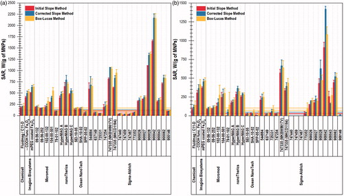
Based on the results of the one-way ANOVA test, there were several MNP samples that had significantly different SAR values depending on the SAR calculation method (see Table SIII). For example, at 345 kHz SAR values for 10 samples are significantly different at α = 0.05. According to the post-hoc tests, the majority of cases correspond to the difference between ISM and BLM.

Both methods, ISM and CSM, are approximations of the phenomenological BLM method which provides the most accurate calculation of SAR among all three methods. Yet BLM is not a complete model for describing heating of MNPs in an applied AMF as concluded based on the results of graphical residual analysis (Figure 2).

Figure 2. Residual plots (b–e, g–j) for HyperMAG B particles after approximation their heating in an alternating magnetic field with a frequency of 345 kHz with (a) BLM and (f) ISM: (b–e) correspond to BLM; (g–j) correspond to the ISM.

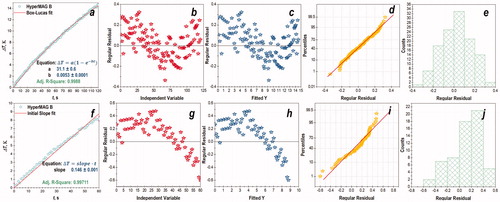
To perform the regression analysis, the data were fitted to the three different models (ISM, CSM, and BLM). The quality of the fitting was judged based on the values of adjusted R², while the validity of the models was assessed using graphical residual analysis (see Figure 2). A visual examination of the residuals was conducted to check for obvious deviations from randomness or the possible presence of heteroscedasticity. The following were used in graphical residual analysis to assess the validity of linear and non-linear fits: (1) scatter plot of the response and predicted values versus the independent variable; (2) scatter plot of the residuals versus the independent variable; (3) scatter plot of the residuals versus the predicted values; (4) histogram of the residuals; and (5) normal probability plot of the residuals [54].

As an example of residual analysis, the plots for HyperMAG B MNPs are depicted in Figure 2. As can be seen from the graphs corresponding to BLM, the residuals are normally distributed around zero (Figure 2(e)), and a normal probability plot of the residuals is approximately linear and has a characteristic slightly s-shaped appearance (Figure 2(d)). There are no outliers, and the fit looks better using non-linear BLM (Figure 2(a)) rather than its linear approximation ISM (Figure 2(f)); though, for both models a non-random structure (curved pattern) in the residuals can be observed (Figure 2(b, c, g, h)).

3.2. High-SAR MNPS

The top-6 MNPs with the highest SAR values are highlighted in each column in red in Tables 1 and 2. The top 25% MNPs based on average temperature change are listed in Table SII and highlighted in yellow. The ranking of MNPs based on their SAR values marginally depends on magnetic field parameters and SAR units. Sigma-Aldrich 900042 MNPs have the highest BLM-SAR value: 2158.4 ± 110.1 W/(g MNP) at 345 kHz/59 kA/m. These MNPs have an iron content of 977.8 ± 55.4 μg Fe/(mg MNP), a magnetic diameter of 12.8 ± 5.8 nm, a mass magnetization value of 90.7 ± 4.5 emu/(g MNP) at 1 T, a core diameter of 22.9 ± 0.2 nm, and a magnetically dead layer thickness equal to 5.1 ± 2.9 nm. They can be heated by 36.9 ± 2.0 K (see Table SII) in 120 s under AMF application (345 kHz/59 kA/m) at a concentration of 1 mg MNP/ml, indicating that they can be an optimal candidate for MFH treatment.

3.3. ILP values

In addition to the differences in the final results due to the calculation methods, SAR values increase with increasing magnetic field frequency/strength. Thus, the ILP (nH·m²/kg) was calculated to normalize the BLM-SAR values W/(g MNP) measured at two different magnetic fields. The corresponding data can be found in Table SIV and in Figure S3. The ILP values at different field strengths and frequencies are in good agreement within the standard deviation of the mean. Nevertheless, 10 samples were found to have significantly different ILP values between the two field strengths and frequencies (highlighted in blue in Table SIV).

3.4. Other MNP properties and their correlation with SAR values

To better understand heating characteristics of MNPs, the physical and magnetic properties were evaluated and compared with information on MNP properties provided by manufacturer (Table 3). Table 3 contains diameters provided by companies, hydrodynamic diameters measured by DLS and NTA, and the magnetic diameter (Fe₃O₄) found by fitting magnetization curves to the Langevin–Chantrell function. Particle coatings and functional groups, which might affect the MNP properties, are also listed in Table 3. Additionally, the mass magnetization (σ) at 1 T was determined using VSM and presented in Table 3 as well.

Table 3. Parameters of MNPS including the diameter provided by the manufacturer, hydrodynamic diameter evaluated by DLS and NTA, magnetic diameter calculated from magnetic hysteresis loops using Langevin–Chantrell function, and mass magnetization at 1 T.

Company	Product number	Coating and functionalization	Diameter from manufacturer (nm)	Hydrodynamic diameter		Magnetic diameter (nm)	σ at 1 T (emu/g MNPs)
				from DLS (nm)	from NTA (nm)
Chemicell	Fluidmag/C11-D	Starch with –OH groups	100	81.5 ± 11.9	80.8 ± 1.6	10.7 ± 4.2	28.6 ± 1.4
Imagion	-COOH func. Fe3O4	Amphiphilic polymer with –COOH groups	25 (core), 43.1 (HD)	35.0 ± 1.7	38.0 ± 2.8	17.1 ± 9.2	55.5 ± 2.8
Biosystems	mPEG coated Fe3O4	Amphiphilic polymer coated with  mPEG	25 (core), 78.4 (HD)	66.8 ± 8.1	103.4 ± 15.5	16.6 ± 9.3	55.4 ± 2.8
Micromod	09-56-132	Dextran with PEG-COOH groups	130	210.4 ± 10.5	87.4 ± 3.4	8.5 ± 2.4	43.8 ± 2.2
	09-56-252	Dextran with PEG-COOH groups	250	303.7 ± 4.8	109.8 ± 10.4	8.5 ± 2.7	38.1 ± 1.9
	102-00-132	Dextran with –OH groups	130	62.9 ± 1.2	115.1 ± 22.6	9.97 ± 10.03	23.7 ± 1.2
	104-00-501	Dextran with –OH groups	50	54.5 ± 1.8	94.7 ± 9.5	16.7 ± 8.4	42.1 ± 2.1
	79-01-102	Dextran with –NH2 groups	100	50.0 ± 8.0	44.7 ± 4.9	9.9 ± 4.4	35.9 ± 1.8
nanoTherics	HyperMAG A	Meso-2,3-dimercaptosuccinic acid	10.3 (core), 100 (HD)	191.0 ± 35.2	101.8 ± 9.2	8.3 ± 1.5	54.7 ± 2.7
	HyperMAG B	Meso-2,3-dimercaptosuccinic acid	11.7 (core), 100 (HD)	150.3 ± 21.4	117.0 ± 13.9	9.0 ± 2.5	90.5 ± 4.0
	HyperMAG C	Meso-2,3-dimercaptosuccinic acid	15.2 (core), 100 (HD)	258.6 ± 59.3	77.9 ± 21.5	9.8 ± 4.3	80.0 ± 4.0
Ocean NanoTech	SEI-10-05	PEI coated	10 (TEM)	71.5 ± 7.0	77.9 ± 2.0	8.7 ± 1.1	34.6 ± 1.7
	SHA-10-02	With –NH2 groups	30	35.1 ± 2.3	44.8 ± 18.2	10.4 ± 2.2	50.4 ± 2.5
	SPP-05-02	With PEG-COOH groups	5	38.4 ± 2.0	33.4 ± 2.7	6.9 ± 4.6	73.7 ± 3.7
Sigma-Aldrich	544884^a	N/a, powder	<50 (BET)	123.7 ± 11.5	96.7 ± 10.0	n/a	40.3 ± 2.0
	637149	N/a, powder	<50 (APS)	n/a, not stable	n/a, not stable	n/a	13.8 ± 0.7
	725331	PEG coated	4-6 (TEM)	59.5 ± 18.0	65.3 ± 6.8	4.2 ± 1.5	3.2 ± 0.1
	747254	With –COOH groups	10 (TEM)	50.4 ± 8.2	125.3 ± 2.1	9.5 ± 1.8	74.7 ± 3.7
	747335^a	With –COOH groups	30 (TEM)	46.4 ± 8.4	63.4 ± 7.0	10.8 ± 2.8	71.9 ± 3.6
	747335^b	With –COOH groups	30 (TEM)	57.1 ± 12.3	77.6 ± 0.6	10.7 ± 3.6	46.7 ± 2.3
	747440	N-succinimidyl ester groups	5 (TEM)	32.9 ± 5.0	51.9 ± 1.1	n/a	0.0 ± 0.1
	747459	N-succinimidyl ester groups	10 (TEM)	30.4 ± 2.8	41.2 ± 30.8	n/a	1.7 ± 0.1
	747467	N-succinimidyl ester groups	30 (TEM)	44.0 ± 4.5	49.9 ± 3.0	n/a	0.6 ± 0.1
	773352	n/a, powder	30 (TEM)	n/a, not stable	44.1 ± 9.3	n/a	2.3 ± 0.1
	900026	PEG coated	15 (TEM)	31.3 ± 4.3	48.4 ± 4.3	12.9 ± 3.6	92.5 ± 4.6
	900027	PEG coated	25 (TEM)	61.3 ± 6.4	51.4 ± 2.9	11.4 ± 8.4	58.3 ± 2.9
	900028	With –NH2 groups	25 (TEM)	47.2 ± 6.6	66.7 ± 8.5	11.5 ± 4.4	57.9 ± 2.9
	900042	Amphiphilic polymer	25 (TEM)	45.7 ± 0.7	41.0 ± 4.7	12.8 ± 5.8	90.7 ± 4.5
	900043	Amphiphilic polymer	15 (TEM)	28.6 ± 1.3	27.7 ± 8.0	12.6 ± 3.4	71.4 ± 3.6
	900062	Amphiphilic polymer	30 (TEM)	49.6 ± 3.7	58.9 ± 0.6	11.3 ± 3.5	66.6 ± 3.3
	900146	Rhodamine B functionalized	10 (TEM)	32.5 ± 0.4	55.1 ± 5.5	10.4 ± 2.4	24.0 ± 1.2

^a Lot MKBW8617V.

^b Lot MKCD1194.

TEM images and magnetization versus field (M versus H) curves for selected MNPs are depicted in Figure 3. All MNP samples imaged have similar hydrodynamic diameters (DLS) ranging from 45.7 ± 0.6 nm to 57.1 ± 12.3 nm and magnetic diameters (VSM fitting) ranging from 9.9 ± 4.4 to 12.8 ± 5.8. However, the SAR values for these particles change from 95.5 ± 13.8 W/(g MNP) to 2158.4 W/(g MNP) based on the BLM at 345 kHz. The SAR value and core diameter calculated from TEM images are listed in the bottom right corner of the TEM images.

Figure 3. TEM images of MNPs: Micromod 79-01-102 (a); Sigma-Aldrich 747335 lot MKBW1867V(b); Sigma-Aldrich 747335 lot MKCD1194(c); Sigma-Aldrich 900028(d); Sigma- Aldrich 900042 (e); and their magnetic hysteresis loops (f). Inserts: SAR values calculated by the Box- Lucas method at 345 kHz are listed in the lower right corner followed by the TEM core diameters.

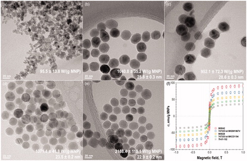
M versus H curves shows that most particles are superparamagnetic in DC fields. Low field plots of MNPs from Figure 3 can be found in Figure S4 and may suggest that a small amount of nanoparticle population can be magnetically blocked. This also includes Sigma-Aldrich MNPs 773352, while 725331, 747440, 747459, and 747467 nanoparticles appear to be paramagnetic. Based on the discrepancy between physical core diameters from TEM and the magnetic diameter calculated from VSM curve fitting with the Langevin–Chantrell function, the magnetically dead layer thickness for each sample was calculated and listed in Table SV.

The correlation coefficients and corresponding p values between BLM-SAR values at 345 kHz/59 kA/m and iron content, hydrodynamic diameter, magnetic diameter, mass magnetization, core diameter, and magnetically dead layer thickness can be found in Table 4. Scatter plots showing the directions and strengths of the correlations can be found in Figure S5.

Table 4. Pearson’s and Spearman s correlation coefficients and its p-values between BLM-SAR values at 345 kHz/59 kA/m and other parameters.

	Pearson's product-moment correlation		Spearman's rank correlation
	Coefficient	p-Value	Coefficient	p-Value
Parameters	SAR (W/(g MNPs))
Iron content (µg Fe/ mg MNPs)	0.50	.00410	0.57	.00086
Hydrodynamic diameter (nm), DLS	−0.06	.74510	0.22	.26208
Magnetic diameter (nm), VSM	0.35	.08270	0.51	.00749
Mass magnetization (emu/g MNPs), VSM	0.57	.00080	0.69	.00002
Core diameter (nm), TEM	0.43	.05017	0.48	.02781
Dead layer thickness (nm), TEM and VSM	0.59	.01247	0.83	.00004

Two-tailed test of significance has been used; parameters significantly (at the 0.05 level) and positively correlated are highlighted in blue; correlation coefficients were rounded to the nearest hundred.

The iron content, mass magnetization, and magnetically dead layer thickness were found to have significant and positive correlations with SAR values based on Pearson’s and Spearman’s correlation coefficients. The magnetic diameter and the core diameter were found to have a significant and positive correlation with SAR values based on Spearman’s correlation coefficient alone. Based on Spearman’s correlation coefficients, in most cases the correlations are moderate (0.50–0.69 range) and moderate to low (0.30–0.49 range), with the strong correlation between SAR and magnetically dead layer thickness (0.83).

4. Discussion

4.1. SAR values and calculation methods (ISM, CSM, and BLM)

Determined SAR values for MNPs often vary between labs due to poor standardization of methodology and measurement conditions. Therefore, the goal of this study was to compare a wide variety of MNPs under the same conditions. In addition, companies often do not provide detailed information on physicochemical, colloidal, and magnetic properties of MNPs, with SAR, in particular, being rarely reported. Thus, an extensive evaluation and characterization of 31 commercial MNPs including SAR (measured at two different AMFs), ILP, and physical and magnetic properties was performed to help to guide researchers in identifying the optimal MNPs for their studies. As a result, the top-6 MNPs highlighted in red in Tables 1 and 2 were identified as great candidates for SAR applications. Among evaluated MNPs, Sigma-Aldrich 900042 MNPs have the highest BLM-SAR value equal to 2158.4 ± 110.1 W/(g MNP) at 345 kHz/59 kA/m. It should be noted that only one batch of MNPs was evaluated for each product besides Sigma-Aldrich 747335 (which had two batches evaluated), and batch variation may exist.

This work will add to the current body of literature available that analyzes SAR of MNPs. An evaluation of other SAR studies in the literature was performed to show comparison of previously studied MNPs. SAR values for iron oxide MNPs and their synthesis methods can be found in review [55], which includes a table of SAR values from the literature. Other studies which examined a variety of commercial MNPs reported maximum ILP values of 3.12 nHm²/kg at 900 kHz/5.5 kA/m for Micromod Nanomag-D-spio Carboxyl MNPs [32] and ∼2 nHm²/kg at 765 kHz/20 kA/m for Chemicell FluidMAG-DX 100 nm MNPs [31] which were not evaluated in our study, however, our highest ILP value was 1.9 ± 0.2 nHm²/kg for Sigma-Aldrich 900042 MNPs at 223 kHz/41 kA/m. Bordelon et al. [56] analyzed three types of MNPs at various AMF conditions and reported the maximum BLM-SAR value equal to 280 ± 130 W/(g Fe) at 150 kHz/40 kA/m for Micromod BNF-Starch MNPs, whereas in our study at 223 kHz/41 kA/m the highest BLM-SAR value was 1108.3 ± 167.6 W/(g Fe) for the Sigma-Aldrich 900042 MNPs. Another study synthesized bionized ferrite MNPs for increased MFH potential with a maximum SAR value of 437 W/(g Fe) by ISM at 153 kHz/57 kA/m [38] (compared with maximum Sigma-Aldrich 544884 SAR value 2129.8 ± 841.5 W/(g Fe) by ISM at 345 kHz/59 kA/m – note the higher frequency). Among the highest SAR values for synthetic MNPs reported in the literature is 1650 W/(g iron oxide) by the ISM at 31 kA/m and 700 kHz [57] and 600 W/g (g of material and calculation method not specified) at 11 kA/m and 410 kHz [58], corresponding to ILP values of 3.8 nHm²/kg and 11.7 nHm²/kg, respectively [32]. In addition to MFH, photothermal therapy using nanoparticles is a promising approach for hyperthermia studies. One study used a panel of non-commercial nanoparticles to compare MFH and photothermal therapy and showed a maximum SAR value of ∼1000 W/(g Fe) for MFH using iron oxide nanocubes at 900 kHz/19 kA/m, and 1.4 mg Fe/mL and ∼12,000 W/(g Au) for photothermal therapy using gold nanorods at 808 nm, 1 W/cm², and 0.15 mg Au/mL [59]. This study [59] also compared heating properties of nanoparticles within an aqueous environment, inside cells, and within tumors, and showed that MNPs lose heating power when internalized by cells.

Despite similarities to ILP and SAR values from the literature, the experimental set-ups for heating measurements can have potential sources of error [18,60,61], with sample volume being one of them. In a few studies [18,60] it was shown that decreasing sample volumes results in lower SAR values. However, it remains unclear if the sample volume effect is statistically significant given that the SAR values were reported without standard uncertainty. Furthermore, another study showed that smaller sample volumes (0.25 mL) have lower rates of heat loss compared to larger volumes (1.0 mL) [12]. Apart from that, conduction losses and energy storage within the sample holders and different sample geometries were discussed as a potential source of error as well [12,60]. Additionally, it has been shown that the location of the temperature probe can have an effect on the SAR value [12,18,60]. Standardization and calibration of experimental set-up for SAR measurements using non-adiabatic systems is further discussed in references [12,62].

In our study, consistent volumes, sample vials, and temperature probe placement were used to minimize these potential sources of error. Additionally, the sample vials were placed in exactly the same location (center) within the solenoid coil using custom 3D printed sample holders. It is important to note that water control samples in our study showed insignificant heating (Table SII). The standard uncertainty for SAR measurements was less than 20% and also accounted for the error propagation during SAR measurements. Higher uncertainty in some samples can be explained by poor colloidal stability of MNP dispersions, especially upon heating, which resulted in poor reproducibility of heating curves for a few samples. Some MNPs quickly aggregated during heating (e.g. Sigma-Aldrich 544884 and 747459), whereas most MNPs remained stable during the measurements.

The SAR calculation methods were found to have a significant effect on its value based on the results of the one-way ANOVA test (Table SIII). Thus, it is crucial for the calculation method of SAR to be reported by other scientists. Between the three methods (ISM, CSM, and BLM) used for SAR calculation, the BLM provides the most accurate SAR estimation for the non-adiabatic system based on the results of graphical residual analysis. The ISM assumes only linear increases in sample temperature and ignores heat losses, while the CSM and BLM both include linear losses due to a non-adiabatic experimental set-up. The first two methods, ISM and CSM, are linear approximations of the phenomenological BLM and can be used in certain situations. ISM would be accurate for adiabatic measurements with no chemical or physical changes within the samples [61].

It should also be noted that different time intervals for ISM-SAR calculation have been used in literature and can affect its accuracy [18,61]. In this study, we chose 60 s time interval since the initial temperature rise was linear within this region for most MNPs. A study by Bordelon et al. [56] has established a protocol for empirically determining appropriate fitting intervals for the ISM to achieve results comparable to the BLM; however, it was only performed for three MNP types and would need to be studied in more detail to ensure it will be accurate for variety of MNPs. This method was further developed by Soetart et al. [61] to identify time ranges of heating which satisfy quasi-adiabatic conditions and it was discussed that an arbitrary choice of a single time interval will likely result in unreliable results. SAR calculation methods are also evaluated by Wildeboer et al. [12] and they found BLM and CSM to give more accurate SAR values than the ISM. However, this study [12] suggested that CSM gives the most accurate results because CSM-SAR values were higher than BLM-SAR value for the selected sample (28 mg/mL Ferucarbotran) even though there is no direct connection between absolute values and model validity.

Herein, we used the graphical residual analysis (see Figure 2) described in Section 3.1 to validate ISM and BLM. However, as one can find in literature, many authors comparing various models often claim a model to be better/worse than others based only on marginal differences in correlation coefficients. However, using R² or adjusted R² is not sufficient and Anscombe's quartet is a good illustration for this point. Besides, the value of R² depends on the degrees of freedom. It means that by simply adding variables to a data set, one can increase the value of R², but this does not improve a fit. To exclude this effect, adjusted R² can be used instead. Further, R², measures only the percentage of variance explained by the data and does not tell us anything about “strength of relationship” or “goodness of a model." Even though it does measure goodness of a fit, R² does not determine the goodness of a model overall. Therefore, it is necessary to diagnose the regression results and validate the tested models using the residual analysis, either graphical or quantitative.

The adjusted R² values for both models (ISM and BLM) shown in Figure 2 are very close to 1 and suggest a good fit for both models. Even though the BLM is the more accurate model compared to ISM as judged by visual examination of residuals, the observed trend in the scatter plot of the residuals versus independent/predicted variables indicates that the BLM is not complete. This leaves room for the development of more comprehensive models for SAR calculations based, for example, on non-linear heat losses [63].

Overall, the results of this study underline the importance of standardizing SAR calculation method. For the case of non-adiabatic systems, which are predominantly used in the literature [61], it is recommended that the BLM to be the method of choice for SAR calculation. Besides the calculation methods, the units for reporting SAR play an important role as well and the SAR values expressed as W/(g MNP) differ from values expressed as W/(g Fe). Until the method for SAR calculations and units is standardized, it is recommended that scientists provide both values in W/(g MNP) and W/(g Fe). The SAR value in W/(g MNP) is more indicative of the heat generation by the sample and it is known in most cases; thus, it should be the chosen annotation as it more accurately represents the heating that will be achieved in real-world applications. SAR values calculated as W/(g MNP) were generally lower than the SAR values calculated as W/(g Fe). Due to low iron content (approximately less than 50 µg Fe/(mg MNP)) and error propagation during calculation, SAR values reported in W/(g Fe) sometimes can have high standard uncertainty which makes such SAR values ambiguous and less precise. Thus, one can obtain a misleading result: samples which generate almost no heat will have high SAR values in W/(g Fe) if they have a low iron content (e.g. Sigma-Aldrich 747440, 747459, and 747467).

4.2. ILP values

The ILP, which corrects SAR for extrinsic parameters, field strength and frequency, was calculated for two measured field strengths and frequencies for each MNP. In general, the ILP (Figure S3) did a sufficient job at normalizing the SAR values, even though significant differences were found for 10 of the evaluated MNPs.

The ILP values must be taken with reservations due to the narrow domain of validity for the relationship $\text{SAR α f}·{\mathrm{H}}_0^2\mathrm{ }$[8,33,56,64]. Carrey et al. [10] examined the domain of validity for the linear response theory that this relationship is based upon and showed that it is mainly useful for highly anisotropic MNPs. As mentioned in the methods section, the ILP parameter is only valid for frequencies up to several hundred MHz, samples with a dispersity of more than 0.1, and field strengths well below the saturation field of the MNPs [32]. In addition, to compare results between different systems, similar environmental thermodynamic losses must be involved [32]. Further, the ILP parameter is only valid for single domain nanoparticles and cannot be used to compare single domain versus multi-domain particles.

4.3. Other MNP properties and their correlation with SAR

MNP properties including iron content, hydrodynamic diameters, magnetic diameters, mass magnetization, core diameters, and thickness of the magnetically dead layer were determined for all samples in order to find correlations with SAR. Identification of any specific properties of the MNPs with high SAR values may have a pivotal impact on the development of the next generation of MNPs for hyperthermia. Importantly, correlations between SAR and iron content (moderate), magnetic diameter (moderate), mass magnetization (moderate), core diameter (moderate to low), and thickness of the magnetically dead layer (strong) were found.

According to the existing models for MNP heating, differences in heat production arise for different MNPs due to their size and anisotropy, and the interplay between size and anisotropy is crucial [8]. Anisotropy can arise from numerous aspects of the MNPs including magnetocrystalline, shape, or colloidal anisotropy [8]. The optimal value/range for MNP size and anisotropy is dependent on field amplitude and frequency; for a given frequency and size, heat generation will increase with anisotropy until the anisotropy field is greater than the magnetic field [8]. Thus, there is a “sweet spot” for the ratio between the anisotropy and magnetic diameter for each magnetic field/frequency combination. This agrees with the findings that correlated magnetic diameter and core diameter with SAR. Other parameters for which correlations with SAR were found including iron content, mass magnetization, and thickness of the magnetically dead layer will have important effects on the anisotropy of the MNPs. Anisotropy can arise from numerous aspects of the MNPs including magnetocrystalline, shape, or colloidal anisotropy [8].

Microscopy (TEM) was used to elucidate whether the core shape and size is responsible for the discrepancies in SAR values. As one can see in Figure 3(a), Micromod particles 79-01-102 with SAR value of 95.5 ± 13.8 W/(g MNP) have an irregular shape which would lead to high shape anisotropy. For a given frequency/field strength, if the anisotropy field is higher than the magnetic field, the MNPs will not produce heat [8]. While it was difficult to discern the exact core size for the Micromod particles 79-01-102, it is clearly smaller than the core size for the rest of MNPs imaged with TEM, which ranged from 22.9 ± 0.2 nm to 28.8 ± 0.3 nm.

All other MNPs depicted in Figure 3 have relatively high SAR values and appear euhedral. The facets on the MNPs could contribute to anisotropy effects or to enhanced chain aggregation effects (i.e. colloidal anisotropy). Work by Martinez-Boubeta et al. has shown that single domain iron oxide nanocubes provide improved magnetic heating efficiency compared to spherical MNPs of analogous sizes, which was attributed to the increased anisotropy of the cubic MNPs and their tendency to aggregate into chains due to the cubic shape [65]. It remains unclear whether the euhedral shape found in the commercial particles is beneficial to SAR or not as it was found in all imaged samples and needs to be studied further. Further, a recent publication by Dennis et al. has shown that differences in heat generation from MNPs with similar size and bulk magnetic properties can be due to variations in the internal magnetic structure that influence coupling of magnetic domains within MNP cores [66].

The magnetically dead layer thickness was calculated by subtracting the magnetic diameter found from fitting of VSM curves to the Langevin function from the core diameter determined from TEM images [46]. A strong positive correlation between SAR values and the magnetically dead layer thickness was observed. Thus, the thickness of the magnetically dead layer might contribute to the anisotropy of the MNPs, even though other studies have stated that a small magnetically dead layer will result in improvement of magnetic performance of the nanoparticles such as saturation magnetization [46,67]. Therefore, this finding needs to be further studied in order to justify the strong correlation found between increased magnetically dead layer thickness and increased SAR value.

5. Conclusions

A comprehensive study of physical and magnetic properties of 31 commercial MNPs including calculation of SAR and ILP was performed. High-SAR MNPs such as Sigma-Aldrich 900042, 900028, 747335, 900062, and nanoTherics HyperMAG B were identified and three SAR calculation methods (ISM, CSM, and BLM) were validated using a graphical residual analysis. Based on the results of model validation, it is suggested that other researchers use the non-linear BLM for SAR calculation and express BLM-SAR values in both units: W/(g MNP) and W/(g Fe). Positive correlations (from moderate to strong) between SAR values and other MNP properties were found and discussed in detail. Studied MNP properties, especially the magnetically dead layer thickness, might contribute to the nanoparticle anisotropy and could be responsible for efficient heating of MNPs in an applied AMF.

6. Future directions

Two different batches of Sigma Aldrich 747335 MNPs were evaluated, but the data was not enough to make any comments on the statistical relevance as only two batches were assessed. However, scientists should be aware that batch to batch variability may exist, and should be studied further. Another limitation of the current study is the frequency/field strength products evaluated are outside of the Atkinson’s limit. Atkinson [68] identified that the biological range of AMF applications for humans should have a product of field strength and frequency less than 485 kA/m·kHz. However, this is currently an area of debate as the value can be adjusted for coil diameter, tissue diameter, and electrical conductivity of the tissue [69–71]. As described by Carrião et al. [70], the free current loss is proportional to the square of the distance from the coil axis and thus a better estimation for the critical field for biomedical applications can be found using the equation $\mathrm{Hf}\mathrm{ }<\mathrm{ }(0.150/\mathrm{r})·485$kA/m·kHz. Additionally, field conditions viable for human use could be expanded in the future as coil design is an area of active development.

Moreover, MNP heating studies performed over a range of magnetic field strengths and frequencies can provide important information about the samples [56,61]. Therefore, in future studies, select MNPs will be evaluated at numerous field strengths/frequencies. Further research for the selected MNPs will be performed at lower field strengths to assess their practical use in biomedical applications in addition to MNP testing in cellular and tumor environments as it was done in previous studies [59,72–74]. Preliminary data collected by our lab using commercial MNPs immobilized in composite polymeric microparticles has shown that they continue to produce high amounts of heat when MNP incorporation is less than 1% of the microparticle volume. In addition, preliminary studies using HeLa cells with these commercial MNPs at a concentration of 1 mg MNP/mL showed high heating rates and subsequent cell death. Thus, it is anticipated that the MNPs with the highest SAR values identified in this study will preserve their heating characteristics once internalized by cells. Other parameters that were not studied in this work such as the crystal structure, crystal defects, and purity might also affect MNP heating efficiency and will require further investigation.

Authors' contributions

JD supervised this work. OL and OK performed the analysis and interpretation of data. OL carried out VSM measurements, and with the help of OK, DW, AM, and NG measured the heating of MNPs in two different AMFs. OK characterized MNPs using UV-vis spectroscopy, DLS (together with OL, OT, and CN), and NTA (together with AM). OK and OL together with SS, OT, CN, and NG quantified iron content for MNPs spectrophotometrically using 1,10-phenanthroline assay. OL performed SAR/ILP calculation using CSM, while OK – using ISM (together with OL and AM) and BLM; OL and OK also calculated the linear loss parameters. OL calculated the magnetic diameters from VSM data (with guidance from SS) and core diameter from TEM photos. OK calculated iron content, hydrodynamic diameters, magnetization at 1 T (together with OL), correlation coefficients (together with OL), and performed graphical residual analysis. OL and OK performed statistical data analysis, and developed methodology and sample preparation techniques. All authors proofread the document and approved the final version.

Acknowledgments

All authors thank Carlos Rinaldi for sharing the following equipment used in this research: EasyHeat™ induction heater (Ambrell, Rochester, NY), ZetaPALS DLS analyzer (Brookhaven Instruments), and NanoSight LM14 NTA analytical software (Malvern Instruments), and for valuable comments, result discussions, and proofreading. We also thank Eric Fuller for providing training on using the induction heater and DLS equipment; David Arnold for sharing the VSM software (ADE Technologies EV9 VSM); and Camilo Velez for providing training for using the VSM. Authors also thank the Research Services Center at the Herbert Wertheim College of Engineering for providing access to the FEI Tecnai F20 S/TEM microscope and Nicholas G. Rudawski for help in operating the microscope. The authors also thank Kyle Allen for providing guidance on statistical analyses, Jennifer Andrew for proofreading the manuscript and giving valuable advice, and Alexander Liptak for his help with the literature search and DLS and spectrophotometry measurements. We also thank Patricia Carothers for grammatical editing. Finally, the authors thank Sigma-Aldrich and Chemicell (Berlin, Germany) for providing samples of MNPs for evaluation.

Disclosure statement

The authors declare that we have no competing interests.

Correction Statement

This article has been republished with minor changes. These changes do not impact the academic content of the article.

References

- Gas P. Essential facts on the history of hyperthermia and their connections with electromedicine. Prz Elektrotechniczny. 2011:87:37–40.
- Hornback NB. Historical aspects of hyperthermia in cancer therapy. Radiol Clin North Am. 1989;27:481–488.
- Thiesen B, Jordan A. Clinical applications of magnetic nanoparticles for hyperthermia. Int J Hyperthermia. 2008;24:467–474.
- Sardari D, Verg N. Cancer treatment with hyperthermia. In: Ozdemir O, editor. Current cancer treatment – novel beyond conventional approaches. Rijeka, Croatia: InTech; 2011. p. 454–474.
- Behrouzkia Z, Joveini Z, Keshavarzi B, et al. Hyperthermia: how can it be used? Oman Med J. 2016;31:89–97.
- Gilchrist RK, Medal R, Shorey WD, et al. Selective inductive heating of lymph nodes. Ann Surg. 1957;146:596–606.
- Kozissnik B, Dobson J. Biomedical applications of mesoscale magnetic particles. MRS Bull. 2013;38:927–932.
- Dennis CL, Ivkov R. Physics of heat generation using magnetic nanoparticles for hyperthermia. Int J Hyperthermia. 2013;29:715–729.
- Pankhurst QA, Connolly J, Jones SK, et al. Applications of magnetic nanoparticles in biomedicine. J Phys D: Appl Phys. 2003;36:R167–R181.
- Carrey J, Mehdaoui B, Respaud M. Simple models for dynamic hysteresis loop calculations of magnetic single-domain nanoparticles: application to magnetic hyperthermia optimization. J Appl Phys. 2011;109:1–17.
- Luo S, Wang L, Ding W, et al. Clinical trials of magnetic induction hyperthermia for treatment of tumours. OA Cancer. 2014;2:2.
- Wildeboer RR, Southern P, Pankhurst QA. On the reliable measurement of specific absorption rates and intrinsic loss parameters in magnetic hyperthermia materials. J Phys D Appl Phys. 2014;47:14.
- Pankhurst QA, Thanh NKT, Jones SK, et al. Progress in applications of magnetic nanoparticles in biomedicine. J Phys D: Appl Phys. 2009;42:1–15.
- Jordan A, Scholz R, Wust P, et al. Magnetic fluid hyperthermia (MFH): cancer treatment with AC magnetic field induced excitation of biocompatible superparamagnetic nanoparticles. J Magn Magn Mater. 1999;201:413–419.
- Néel L. Influence des fluctuations thermiques a l’aimantation des particules ferromagnétiques. C R Acad Sci. 1949;228:664–668.
- Rosensweig RE. Heating magnetic fluid with alternating magnetic field. J Magn Magn Mater. 2002;252:370–374.
- Cruz MM, Ferreira LP, Alves AF, et al. Nanoparticles for magnetic hyperthermia. Nanostructures Cancer Ther. 2017;105:485–511.
- Wang SY, Huang S, Borca-Tasciuc DA. Potential sources of errors in measuring and evaluating the specific loss power of magnetic nanoparticles in an alternating magnetic field. IEEE Trans Magn. 2013;49:255–262.
- Zhao X, Kim J, Cezar CA, et al. Active scaffolds for on-demand drug and cell delivery. Proc Natl Acad Sci U S A. 2011;108:67–72.
- Lanier OL, Monsalve AG, McFetridge PS, et al. Magnetically triggered release of biologics. Int Mater Rev. 2019;64:63–90.
- Fuller EG, Sun H, Dhavalikar RD, et al. Externally triggered heat and drug release from magnetically controlled nanocarriers. ACS Appl Polym Mater. 2019;1:211–220.
- Monsalve A, Carolina A, Rinaldi C, et al. Remotely triggered activation of TGF- β with magnetic nanoparticles. IEEE Magn Lett. 2015;6:1–5.
- Ceylan S, Coutable L, Wegner J, et al. Inductive heating with magnetic materials inside flow reactors. Chem Eur J. 2011;17:1884–1893.
- Chen R, Romero G, Christiansen MG, et al. Wireless magnetothermal deep brain stimulation. Science. 2015;347:1477–1480.
- Gaitas A, Kim G. Inductive heating kills cells that contribute to plaque: a proof-of-concept. PeerJ. 2015;3:e929.
- Mathieu JB, Martel S. Aggregation of magnetic microparticles in the context of targeted therapies actuated by a magnetic resonance imaging system. J Appl Phys. 2009;106:044904.
- Wabler M, Zhu W, Hedayati M, et al. Magnetic resonance imaging contrast of iron oxide nanoparticles developed for hyperthermia is dominated by iron content. Int J Hyperthermia. 2014;30:192–200.
- Angelakeris M, Li Z-A, Sakellari D, et al. Can commercial ferrofluids be exploited in AC magnetic hyperthermia treatment to address diverse biomedical aspects? EPJ Web Conf. 2014;75:08002–08004.
- Maier-Hauff K, Ulrich F, Nestler D, et al. Efficacy and safety of intratumoral thermotherapy using magnetic iron-oxide nanoparticles combined with external beam radiotherapy on patients with recurrent glioblastoma multiforme. J Neurooncol. 2011;103:317–324.
- Shinkai M, Yanase M, Suzuki M, et al. Intracellular hyperthermia for cancer using magnetite cationic liposomes. J Magn Magn Mater. 1999;194:176–184.
- Sakellari D, Mathioudaki S, Kalpaxidou Z, et al. Exploring multifunctional potential of commercial ferrofluids by magnetic particle hyperthermia. J Magn Magn Mater. 2015;380:360–364.
- Kallumadil M, Tada M, Nakagawa T, et al. Suitability of commercial colloids for magnetic hyperthermia. J Magn Magn Mater. 2009;321:1509–1513.
- Andreu I, Natividad E. Accuracy of available methods for quantifying the heat power generation of nanoparticles for magnetic hyperthermia. Int J Hyperthermia. 2013;29:739–751.
- Chou CK. Use of heating rate and specific absorption rate in the hyperthermia clinic. Int J Hyperthermia. 1990;6:367–370.
- Piñeiro-Redondo Y, Bañobre-López M, Pardiñas-Blanco I, et al. The influence of colloidal parameters on the specific power absorption of PAA-coated magnetite nanoparticles. Nanoscale Res Lett. 2011;6:383.
- Yuan Y, Tasciuc D-A. Comparison between experimental and predicted specific absorption rate of functionalized iron oxide nanoparticle suspensions. J Magn Magn Mater. 2011;323:2463–2469.
- Majeed J, Pradhan L, Ningthoujam RS, et al. Enhanced specific absorption rate in silanol functionalized Fe3O4 core–shell nanoparticles: study of Fe leaching in Fe3O4 and hyperthermia in L929 and HeLa cells. Colloids Surf B Biointerfaces. 2014;122:396–403.
- Grüttner C, Müller K, Teller J, et al. Synthesis and antibody conjugation of magnetic nanoparticles with improved specific power absorption rates for alternating magnetic field cancer therapy. J Magn Magn Mater. 2007;311:181–186.
- Zhang L-Y, Gu H-C, Wang X-M. Magnetite ferrofluid with high specific absorption rate for application in hyperthermia. J Magn Magn Mater. 2007;311:228–233.
- Guardia P, Di Corato R, Lartigue L, et al. Water-soluble iron oxide nanocubes with high values of specific absorption rate for cancer cell hyperthermia treatment. ACS Nano. 2012;6:3080–3091.
- Corrected slope SAR and ILP analysis programmes, written in Microsoft Excel and Matlab formats. [cited 2019 Jun 15]. Available from: www.resonantcircuits.com.
- Ortega D, Pankhurst QA. Magnetic hyperthermia. In: O’Brien P, editor. Nanoscience: Volume 1: Nanostructures through Chemistry. Cambridge: Royal Society of Chemistry; 2013; 60–88.
- ASTM E394-15. Standard test method for iron in trace quantities using the 1,10 phenanthroline method. West Conshohocken, PA: ASTM International; 2015.
- De Jaeger N, Demeyere H, Finsy R, et al. Particle sizing by photon correlation spectroscopy part I: monodisperse latices: influence of scattering angle and concentration of dispersed material. Part Part Syst Charact. 1991;8:179–186.
- NIST e-Handbook of Statistical Methods 1.3.6.6.9. Lognormal Distribution. [cited 2019 Jun 15]. Available from: http://www.itl.nist.gov/div898/handbook/eda/section3/eda3669.htm.
- Unni M, Uhl AM, Savliwala S, et al. Thermal decomposition synthesis of iron oxide nanoparticles with diminished magnetic dead layer by controlled addition of oxygen. ACS Nano. 2017;11:2284–2303.
- Chantrell R, Popplewell J, Charles S. Measurements of particle size distribution parameters in ferrofluids. IEEE Trans Magn. 1978;14:975–977.
- Ferguson RM, Minard KR, Khandhar AP, et al. Optimizing magnetite nanoparticles for mass sensitivity in magnetic particle imaging. Med Phys. 2011;38:1619–1626.
- Ma J, Chen K. Magnetic dead layer is not “magnetically dead” in hematite nanocubes. Phys Lett A. 2013;377:2216–2220.
- Kaiser R, Miskolczy G. Magnetic properties of stable dispersions of subdomain magnetite particles. J Appl Phys. 1970;41:1064–1072.
- Taylor BN, Kuyatt CE. Guidelines for evaluating and expressing the uncertainty of NIST measurement results. NIST Tech Note. 1994;1297.
- Ferregut C, Nazarian S, Vennalaganti K, et al. Fast error estimates for indirect measurements: applications to pavement engineering. Reliable Comput. 1996;2:219–228.
- NIST e-Handbook of Statistical Methods 7.4.7.3 Bonferroni’s method. [cited 2019 Jun 15]. Available from: https://www.itl.nist.gov/div898/handbook/prc/section4/prc473.htm.
- Samchenko Y, Korotych O, Kernosenko L, et al. Stimuli-responsive hybrid porous polymers based on acetals of polyvinyl alcohol and acrylic hydrogels. Colloids Surf A Physicochem Eng Asp. 2018;544:91–104.
- Grüttner C, Müller K, Teller J, et al. Synthesis and functionalisation of magnetic nanoparticles for hyperthermia applications. Int J Hyperthermia. 2013;29:777–789.
- Bordelon DE, Cornejo C, Grüttner C, et al. Magnetic nanoparticle heating efficiency reveals magneto-structural differences when characterized with wide ranging and high amplitude alternating magnetic fields. J Appl Phys. 2011;109:124904–124908.
- Fortin JP, Wilhelm C, Servais J, et al. Size-sorted anionic iron oxide nanomagnets as colloidal mediators for magnetic hyperthermia. J Am Chem Soc. 2007;129:2628–2635.
- Hergt R, Hiergeist R, Hilger I, et al. Maghemite nanoparticles with very high AC-losses for application in RF-magnetic hyperthermia. J Magn Magn Mater. 2004;270:345–357.
- Espinosa A, Kolosnjaj-Tabi J, Abou-Hassan A, et al. Magnetic (hyper)thermia or photothermia? Progressive comparison of iron oxide and gold nanoparticles heating in water, in cells, and in vivo. Adv Funct Mater. 2018;28:1803660.
- Huang S, Wang SY, Gupta A, et al. On the measurement technique for specific absorption rate of nanoparticles in an alternating electromagnetic field. Meas Sci Technol. 2012;23:1–6.
- Soetaert F, Kandala SK, Bakuzis A, et al. Experimental estimation and analysis of variance of the measured loss power of magnetic nanoparticles. Sci Rep. 2017;7:1–15.
- Attaluri A, Nusbaum C, Wabler M, et al. Calibration of a quasi-adiabatic magneto-thermal calorimeter used to characterize magnetic nanoparticle heating. J Nanotechnol Eng Med. 2013;4:011006–011008.
- Coïsson M, Barrera G, Celegato F, et al. Specific absorption rate determination of magnetic nanoparticles through hyperthermia measurements in non-adiabatic conditions. J Magn Magn Mater. 2016;451:2–7.
- Soto-Aquino D, Rinaldi C. Nonlinear energy dissipation of magnetic nanoparticles in oscillating magnetic fields. J Magn Magn Mater. 2015;393:46–55.
- Martinez-Boubeta C, Simeonidis K, Makridis A, et al. Learning from nature to improve the heat generation of iron-oxide nanoparticles for magnetic hyperthermia applications. Sci Rep. 2013;3:1652.
- Dennis CL, Krycka KL, Borchers JA, et al. Internal magnetic structure of nanoparticles dominates time-dependent relaxation processes in a magnetic field. Adv Funct Mater. 2015;25:4300–4311.
- Issa B, Obaidat IM, Albiss BA, et al. Magnetic nanoparticles: surface effects and properties related to biomedicine applications. IJMS. 2013;14:21266–21305.
- Atkinson WJ, Brezovich IA, Chakraborty DP. Usable frequencies in hyperthermia with thermal seeds. IEEE Trans Biomed Eng. 1984;31:70–75.
- Kozissnik B, Bohorquez AC, Dobson J, et al. Magnetic fluid hyperthermia: advances, challenges, and opportunity. Int J Hyperthermia. 2013;29:706–714.
- Carrião MS, Aquino VRR, Landi GT, et al. Giant-spin nonlinear response theory of magnetic nanoparticle hyperthermia: a field dependence study. J Appl Phys. 2017;121:173901–173913.
- Wust P, Gneveckow U, Johannsen M, et al. Magnetic nanoparticles for interstitial thermotherapy − feasibility, tolerance and achieved temperatures. Int J Hyperthermia. 2006;22:673–685.
- Dennis CL, Jackson AJ, Borchers JA, et al. Nearly complete regression of tumors via collective behavior of magnetic nanoparticles in hyperthermia. Nanotechnology. 2009;20:395103–395115.
- Dutz S, Kettering M, Hilger I, et al. Magnetic multicore nanoparticles for hyperthermia-influence of particle immobilization in tumour tissue on magnetic properties. Nanotechnology. 2011;22:265102–265101.
- Giustini AJ, Ivkov R, Hoopes PJ. Magnetic nanoparticle biodistribution following intratumoral administration. Nanotechnology. 2011;22:345101–345101.