Proton range uncertainty caused by synthetic computed tomography generated with deep learning from pelvic magnetic resonance imaging

Abstract

Background

In proton therapy, it is disputed whether synthetic computed tomography (sCT), derived from magnetic resonance imaging (MRI), permits accurate dose calculations. On the one hand, an MRI-only workflow could eliminate errors caused by, e.g., MRI-CT registration. On the other hand, the extra error would be induced due to an sCT generation model. This work investigated the systematic and random model error induced by sCT generation of a widely discussed deep learning model, pix2pix.

Material and Methods

An open-source image dataset of 19 patients with cancer in the pelvis was employed and split into 10, 5, and 4 for training, testing, and validation of the model, respectively. Proton pencil beams (200 MeV) were simulated on the real CT and generated sCT using the tool for particle simulation (TOPAS). Monte Carlo (MC) dropout was used for error estimation (50 random sCT samples). Systematic and random model errors were investigated for sCT generation and dose calculation on sCT.

Results

For sCT generation, random model error near the edge of the body (∼200 HU) was higher than that within the body (∼100 HU near the bone edge and <10 HU in soft tissue). The mean absolute error (MAE) was 49 ± 5, 191 ± 23, and 503 ± 70 HU for the whole body, bone, and air in the patient, respectively. Random model errors of the proton range were small (<0.2 mm) for all spots and evenly distributed throughout the proton fields. Systematic errors of the proton range were −1.0(±2.2) mm and 0.4(±0.9)%, respectively, and were unevenly distributed within the proton fields. For 4.5% of the spots, large errors (>5 mm) were found, which may relate to MRI-CT mismatch due to, e.g., registration, MRI distortion anatomical changes, etc.

Conclusion

The sCT model was shown to be robust, i.e., had a low random model error. However, further investigation to reduce and even predict and manage systematic error is still needed for future MRI-only proton therapy.

Keywords:

• MRI-only
• proton range uncertainty
• synthetic CT
• deep learning
• pelvis

Introduction

Conventional proton therapy uses computed tomography (CT) as the standard imaging modality for dose calculation [1]. Recently, it has been proposed to use magnetic resonance imaging (MRI) as an alternative to CT with the potential to improve radiotherapy by exploiting the advantages of MRI, e.g., the unparalleled high soft-tissue contrast and the absence of ionising radiation exposure [2]. However, MRI does not provide information on the proton-stopping power required for dose calculation [1]. A strategy to obtain this information is to, first, generate a so-called synthetic CT (sCT) from the MRI and, second, to transfer the sCT into a stopping power ratio (SPR) map.

Besides conventional analytical tools for sCT generation, i.e., bulk density [3–9] and atlas-based [5,6,10–14] methods, deep learning (DL) based methods have shown great potential in terms of, e.g., better adaptation to tissue heterogeneity and lower computational resource requirements [1]. Dose calculation on sCT has been widely investigated for photon radiation, while proton dose has been much less discussed. According to a recent review in 2021 [2], only a comparably small number (9 out of 57) of state-of-the-art studies investigated proton dose on generated sCT [15–23].

Proton and other ion therapies benefit from and are characterised by their dosimetric advantages: a low entrance dose and a distinct dose maximum, called Bragg peak, near the end of their finite beam range. Besides, the linear energy transfer (LET) of a proton beam, which relates to the biological effectiveness [24], also steeply increases near the Bragg peak at the end of the range. The proton range in patients is uncertain due to, e.g., CT number conversion, and intra- and inter-fractional anatomical changes. A safety margin around the target volume has to be applied in proton therapy to consider the uncertainties of the position of Bragg peaks that are placed at the edge of the target volume. The size of the safety margin depends on proton range uncertainty, i.e., large proton range uncertainty leads to the extension of the margin, and thereby, substantially increases the high dose volume in normal tissue. Calculating proton dose on sCT, which is not directly measured but derived from MRI using models, would induce extra proton range uncertainties, as the proton range is sensitive to CT number errors. It is important to know and ideally reduce the induced uncertainty caused by sCT generation. Until recently, only a few studies investigated proton range on generated sCT [2] and these were mostly related to brain and head and neck patients [15,16,18,23].

This study focuses on quantifying model-induced proton range errors resulting from sCT generation. For sCT generation, a prototype model of a widely investigated [25–36] conditional generative adversarial network (cGAN), pix2pix [37] was applied. The open-access dataset of Gold Atlas [38] was employed.

Material and methods

Patient data

This study used MRI-CT pairs of nineteen patients with cancer in the pelvis acquired by three different Swedish departments. They were used as provided and described by the open-access dataset Gold Atlas, which was initiated for the purpose of establishing segmentation and sCT generation methods [38]. In brief, the number of patients contributed by department 1, 2 and 3 are eight, seven, and four, respectively. The MRI images of departments 1, 2 and 3 were obtained with different machines, namely, 3 T GE Discovery, 1.5 T Siemens, and 3 T GE Signa, respectively [38]. Correspondingly, CT scanners were: Siemens Somatom Definition AS+, Toshiba Aquilion, and Siemens Emotion 6, respectively [38]. Furthermore, the authors deformably registered the CT to the T2-weighted MRI images resulting in a set of two-dimensional (2D) MRI-CT slice pairs for each patient. The deformed and resampled CT and the T2-weighted MRI images both had a voxel size of 0.875 × 0.875 × 2.5 mm³ [38].

In this work, it was assumed that the CT in the dataset was the planning CT on which the treatment plan dose was supposed to be calculated. Thus, the CT and the dose calculated on the CT were regarded as ground truth. For modelling, the nineteen patients were randomly split into training (ten patients, 880 pairs of 2D MRI-CT slices in total), test (five patients, 412 pairs of 2D MRI-CT slices), and validation (four patients, 237 pairs of 2D MRI-CT slices).

Preprocessing

First, all images were converted to have a common image size of 500 × 376 pixels (pixel size unchanged) by adding/removing air-filled areas at the edges of all paired CT and MRI images. The image intensities of MRI images from the three sites were linearly transferred so that the differences between histograms of MRI intensities of the three MR scanners were minimised. Based on the experience of [25], where the same dataset and a similar DL model were used, in this work, the following preprocessing steps were applied to the MRI data: 1) N4ITK bias field correction [39] with parameters of convergence threshold 0.004, number of histogram bins 200, Wiener filter noise 0.01, downsampling 3. 2) A curvature anisotropic diffusion filter was applied with the settings of conductance 1, scaling update interval 1, time step 0.03, iterations 10. The MRI intensities were truncated from 0 to 2165 (98% maximum), i.e., voxels with initial intensities higher than 2165 were set to 2165. For CT images, the intensities were truncated from −600 HU to 1400 HU, as CT numbers below −600 were considered air (and set to −600), and CT numbers above 1400 were identified (and set to 1400) only in a limited number of cases [25]. The percentage of voxels with CT numbers higher than 1400 HU and between −600 HU and −1000 HU in the body of the initial CT before truncation were both less than 0.1%. Afterwards, both MR and CT images were normalised to the range of [-1] for DL modelling.

Model architecture and hyperparameter settings

For the sCT prediction, a cGAN model extension, pix2pix [37], was employed. The original authors observed that this model allows training using a comparably small number of image pairs, e.g., 400 [37]. Different models based on pix2pix have been discussed in some detail elsewhere [25–35] and it was not the intention of this work to make a comparison between those approaches of applying pix2pix. Thus, the prototype architecture of pix2pix was applied. The input and output of the model were MRI and its corresponding CT, both were 3-channel 2D images. The three channels included a central 2D image slice with the two adjacent slices above and below it. Previous work on hyperparameter search showed that different settings of learning rate, number of epochs, and the trade-off λ had no significant improvements over default settings [25]. Thus, confirmed with patients in the validation set, the corresponding default hyperparameters, 2 × 10⁻⁴, 200, 100, respectively, were used.

For training, paired image sections with a size of 256 × 256 pixels (i.e., the default input size for pix2pix) were randomly cropped from the MRI-CT image pairs and then entered into the model. The pix2pix default dropout rate of 50% was applied, i.e., 50% of the nodes were randomly and temporarily excluded during training to avoid overfitting [40]. For model testing, four partially overlapping 256 × 256-pixel image parts, each aligned with a corner of the MRI, were cut from the input MRI and then fed into the model. The resulting four model outputs were combined to produce a full sCT prediction of this MRI. For the pixels where partial images overlapped, averages were taken from the image intensities.

Particle transport simulation for proton range

The tool for particle simulation (TOPAS) [41] was used to simulate the proton irradiation on the real CT and sCT for proton range comparison. A grid of 11 × 11 proton pencil beams (called spots in the following) was simulated. Proton spots were evenly distributed within a square area of 10 × 10 cm² and entered the patient under 90° from the right side. The energy for all spots was set to 200 MeV (proton range in water of about 26 cm), which is usually among the highest energies for clinical treatments. The relative energy spread was set to 0.7 and the lateral spot width was set to 0.65 cm. For each spot, 1 × 10⁵ protons were simulated and a 3D dose distribution was recorded using the dose to water scorer and a dose grid corresponding to the CT grid. The proton range was calculated by the distance between spot entrance into the patient and the 80% distal dose fall-off of the laterally integrated depth dose profile.

Evaluation

In this work, model-induced errors [42–46], i.e., systematic and random model errors, were investigated. The systematic error was estimated by the difference between the estimation of the DL prediction and the reference while the random model error was measured by the standard deviation (STD) of the prediction samples generated from the same input. For this purpose, a Monte Carlo (MC) dropout strategy [47] was employed to generate sCT prediction samples: by applying MC dropout on a trained model, a sub-model with a predefined rate of randomly excluded nodes can be obtained, allowing for an individual complete sCT prediction of an input MRI. MC dropout can be repeated n times to obtain n individual sub-models and sCT predictions for the same MRI. In the following, these sCT predicted by individual sub-models for the same MRI are called sub-sCT. In this work, the dropout rate was set to 50% and for each input MRI, 50 sub-sCT were predicted.

For the sCT generation, the mean of the CT numbers of all sub-sCT in a voxel represents the estimation of the sCT voxel prediction for a given MRI. Likewise, the random model error of an sCT voxel prediction is measured by the STD of the CT numbers of the sub-sCT in this voxel. The systematic error was measured by the mean absolute error (MAE) and mean error (ME) of the CT numbers between the real CT and the estimation of sCT.

For the proton range, the errors associated with the random model error and the systematic error of the prediction were determined. For a proton spot, the proton ranges were simulated on all 50 sub-sCTs and the obtained STD in the range was considered as the random model error of the range for that spot. The systematic error of the range prediction for a proton spot was measured by the difference between its range on the real CT and on the estimation of the sCT, i.e., the mean of the sub-sCT. The Spearman correlation between the systematic proton range error of a spot and the mean along its beam path of 1) the sCT systematic error, 2) the square of the sCT systematic error and 3) the sCT random model error was calculated. Random model error of the proton range was not considered in the correlation analysis as this error was observed to be very small for all proton spots (c.f. Section ‘Model-induced proton range error’').

Results

Model-induced sCT errors

For sCT prediction (example cf. Figure 1), both systematic and random model errors were not uniformly distributed over a slice and were found to be higher at the edges of different (anatomical) objects, especially at the body contour. The random model error at the edge of the patient was much higher (∼200 HU) than in the other considered areas inside the body (mostly less than 10 HU) and also higher than at the bone edges (∼100 HU).

Figure 1. Example of MRI (a), CT (B), and sCT (C) for a corresponding slice, along with associated random model error (i.e., the standard deviation of the 50 sub-sCTs; D) and the systematic error of sCT (i.e., the difference between the CT and the sCT; E).

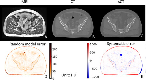
The histograms of the systematic and the random model error (displayed for error values larger than 10 HU) for different areas are shown in Figure 2. The four areas body, bone, air, and edge correspond to the entire region within the body contour, regions with CT numbers of the real CT greater than 250 HU, regions within the body contour with CT numbers smaller than −200 HU, and a band at the body contour with a width of 7 voxels, respectively. The systematic error of body, bone, air, and soft tissue, i.e., all voxels within the body contour except those from the air and bone areas, are listed in Table 1. The systematic error within the body contour in areas with air on the real CT was systematically biased, i.e., the model had difficulties predicting air cavities that are found on the CT based on the given MRI.

Figure 2. Histogram of the (A) random model and (B) systematic error for sCT in the test dataset Separated according to area defined by the CT numbers of the real CT. Relative histograms are shown as the volumes of the considered areas differ substantially. For random model error, data with values < 10 HU are omitted to highlight the behaviour at large errors.

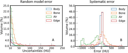
Table 1. The mean absolute error (MAE) and mean error (ME) between the sCT and CT Evaluated separately for the training and test dataset in different areas.

	MAE (HU)				ME (HU)
Dataset	Body	Bone	Air	Soft tissue	Body	Bone	Air	Soft tissue
Training	37 ± 3	138 ± 15	421 ± 88	26 ± 2	1 ± 7	28 ± 27	−409 ± 87	1 ± 5
Test	49 ± 5	191 ± 23	503 ± 70	33 ± 5	12 ± 11	102 ± 41	−494 ± 76	3 ± 10

Model-induced proton range errors

The random model error of the predicted proton range was low (< 0.2 mm) for all spots. It was distributed evenly across the 10 × 10 cm² spot grid (Figure 3A) and comparable for all patients.

Figure 3. Beam’s eye view (BEV) of the (A) random model error and (B) systematic error of proton range of 121 individually simulated lateral 200 MeV proton beams on a 10 × 10 cm² beam grid oriented in anterior-posterior (AP) and cranial-caudal direction (CC) for one patient in the test dataset.

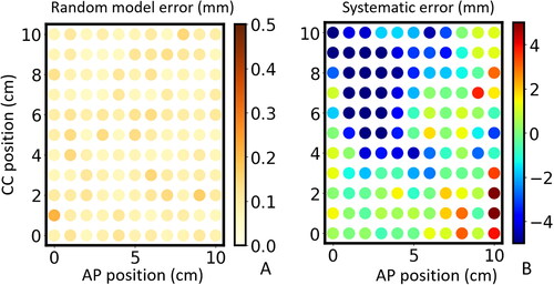
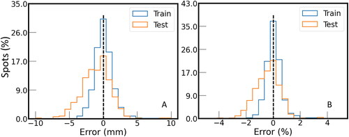
On the other hand, the systematic proton range errors were larger and were not evenly distributed in space (Figure 3B) and varied between patients. Absolute and relative values of systematic proton range errors (± STD) were estimated to be −1.0 (± 2.2) mm and −0.4 (± 0.9)%, respectively, for the test dataset and 0.1 (± 1.6) mm and 0.1 (± 0.6)% for the training dataset, respectively. The median absolute proton range error for the test and training datasets were 1.5 and 0.7 mm, respectively. The histograms of absolute and relative values of systematic proton range errors for all spots are shown in Figure 4A and B, respectively.

Figure 4. Histogram of (A) absolute and (B) relative values of systematic proton range errors of all beams simulated on the training and test dataset. The number of proton beams is normalised.

Figure 5 shows laterally integrated proton depth dose profiles as well as CT and sCT numbers along the beam path for four typical situations that resemble one ideal sCT prediction (I) as well as three predictions (II–IV) resulting in large systematic range errors for the considered spots. The corresponding CT, MRI, and sCT slices for these four proton spots are presented in Figure 6. It can be observed that:

Figure 5. Comparison of the distal part of the laterally integrated dose profiles (A) and corresponding CT number profiles along the beam path (B) of four exemplary proton beams (I-IV) simulated on corresponding CT (red) and sCT (blue) slices.

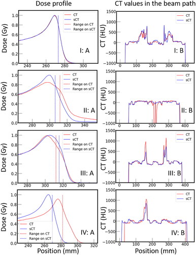
Figure 6. Comparison of CT (a), MRI (B) and corresponding sCT (C) for the same four exemplary patient slices (I-IV) as in Figure 5 with the simulated beam paths indicated as red lines.

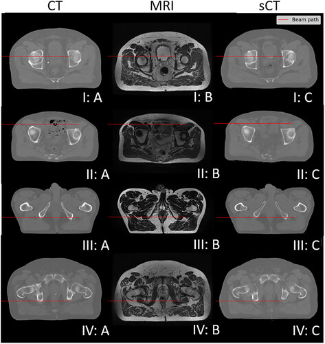
For case I, the depth dose distribution remained unaltered as the small differences between CT and sCT numbers averaged out along the beam path. For case II, air cavities in the CT substantially degraded the Bragg peak but were not predicted on the sCT resulting in a shorter range and steeper distal dose fall-off. For case III, the overall agreement between CT and sCT numbers was good, except for the maximum CT numbers of the sCT in the high-density bone areas, which were predicted to be lower than those in the CT resulting in a less degraded shape of the Bragg peak curve. For case IV, the shape of the sCT was consistent with the MRI but differed, particularly, in the outer regions of the image from the CT. There, the sCT appeared to be stretched, resulting in an effectively shorter proton range in the patient compared to the CT.

Correlation of errors

Spearman correlation between the relative values of systematic proton range error and the mean of the systematic sCT error along the beam path was observed to be −0.78. Low correlations were observed between the systematic proton range errors and the mean of the squared systematic sCT errors as well as the mean of the random sCT errors in the beam path, which are −0.04 and −0.03, respectively.

Discussion

In this work, a cGAN DL model, which showed promising performance for sCT prediction in previous studies [25–35], was trained and tested using the open-source dataset Gold Atlas [38], which contains CT-MRI pairs for 19 patients with cancer in the pelvis. Afterwards, the errors induced by the model were analysed. For the systematic error of sCT generation, the model performance was consistent with that in the previous work by Fetty et al. [25] using the same DL model and dataset. The random model error of sCT prediction was high at the edge of a patient, moderate at the bone edges, and much lower inside the body.

The systematic range errors of 200 MeV proton spots resulting only from the sCT prediction were distributed for the test dataset on the absolute and relative scales as −1.0 (± 2.2) mm and −0.4% (± 0.9)%, respectively. The random model error of the proton range, on the other hand, was found to be much smaller and below 0.2 mm for all beams. The median absolute proton range error was 1.5 mm, while other studies reported a median absolute error in proton range estimation with sCT of 1.7 mm for the liver [22] and 0.5 mm for the brain [48]. Although different models for different anatomical regions and datasets are not directly comparable [1], the errors observed in this work are in the same order of magnitude as those reported in the literature.

For 4.5% and 1.1% of the spots in the test and training dataset, respectively, large systematic proton range errors (more than 5 mm) were observed. These large errors were usually related to, e.g., objects such as low-density air cavities or high-density bone on CT that were not predicted 'correctly’ (cf., Figures 5 and 6, cases II and III), or general mismatch between CT and MRI (case IV). This is consistent with the systematic error maps between CT and sCT, where large errors in CT numbers were found near the boundaries of objects, e.g., between bone, tissue, and air. In accordance with this, random model error maps showed high uncertainty values at the edge of the body contour, i.e., the robustness of the predicted CT numbers is low at the edge of the body. We believe that this is also related to the mismatch in spatial extent, especially near the outer contour, between the CT and MRI in the training dataset. Previous work reported [22] that the sCT predicted by their cycle GAN model matched the associated MRI better than the corresponding real CT, which is consistent with our findings. Future applications of MRI-only proton therapy may benefit if the prediction algorithm generates an sCT that matches the input MRI (e.g., from daily imaging), rather than forcing an sCT geometry that matches that of the original CT, because organ locations and anatomy may differ in between MRI and CT imaging [22]. However, on the one hand, unwanted sCT errors could occur due to possible geometrical distortions or artefacts during MRI reconstruction. On the other hand, anatomical mismatch affects both model training (due to spoiled optimisation of the loss function) and testing (due to imperfect 'ground truth’). This mismatch issue might primarily be mitigated by improving data quality. First, image data pre-processing including accurate spatial distortion correction algorithms for MRI image reconstruction and CT-MRI registration could be improved. Research [49] reported that improved registration had a positive impact on sCT generation model training. Second, the similarity between the underlying MRI and CT images could be increased by minimising the effects of, e.g., setup changes (patient positioning) and anatomical changes (e.g., different gas filling in organs) between image acquisitions. Furthermore, improving the ground truth by using specific MRI sequences that provide better bone contrast is an option. A recent work using a Zero Echo Time (ZTE) MRI sequence, which provides better information on cortical bone and faster scanning times (65 s), achieved MAE (±STD) values within external contour, soft-tissue, and bone of 36 (±3), 7 (±1) and 98 (±14) HU for patients with cancer in the pelvis [50].

Error prediction indicating the confidence of model prediction would help in the future application of DL-based MRI-only proton therapy. A recent study of [42] reported that the square of the prediction error, including systematic error and random error, can be predicted using DL methods. The Spearman correlation between the systematic proton range error and the systematic sCT error was high. However, the correlation between the systematic proton range error and the currently predictable square of the prediction error was low. Future studies concerning the prediction of proton range error are needed.

This work has several limitations. The underlying CT-MRI dataset [38] was taken directly from the literature. MRI sequence selection and preprocessing, e.g., MRI reconstruction and deformable registration remained unchanged. Specifically, the registration strategy may not guarantee an ideal match of all objects on CT and MRI. The CT images were deformably registered using parameter files that were experimentally optimised through visual inspection. Image similarity was measured by mutual information and B-splines were used as a transformation model. The bladder contour delineated by five human experts was used for guidance [38]. Higher sCT errors were found at the edge of the body where a clear mismatch can be observed (cf. Figure 1, Figure 6 case I and IV). To our knowledge, there is no solution available for 'ideal’ pixel-to-pixel registration that allows 'ideal’ match for all objects. Further investigation of registration strategies, e.g., registration based on air-soft tissue-bone instead of clinical delineation, is desired for future development of sCT generation in proton therapy. Besides, more details on, e.g., CT scan voltage and time gap between the acquisition of MRI and CT are missing. These factors might limit the performance of the model. However, as previously suggested by [1], we also believe that keeping the dataset unchanged is useful for direct comparison between our work and potential future work. We avoided applying any extension of the pix2pix model that has been proposed by others [25–36] as most of these extensions were based on a specific dataset and it was not the intention to compare or validate them in this work. We believe that the most important cause of error was the mismatch between MRI and CT, which can hardly be resolved by changes to the model. In addition, the clinical impact of uncertainties, e.g., in patient setup, image acquisition, and CT-SPR conversion, was not quantitatively considered. Besides, the energy of all proton spots was set to 200 MeV, i.e., the spots did not resemble a clinical treatment field and, accordingly, no clinical dose distributions such as dose volume histograms were considered. Our motivation was to focus generally on range errors in sCT of proton spots that could be placed at the distal edge of the target volume in pelvic cases. Instead of sCT, in the future, SPR maps could be directly predicted using MRI and dual energy CT [51] to further reduce range uncertainty in proton beam simulations [52] and, eventually, the necessary dose margins around the target volume.

Conclusion

A cGAN model using an open-source pelvis MRI-CT dataset (Gold Atlas) was trained for uncertainty analysis. Systematic and random model errors of both the generated sCT and proton ranges on the sCT were estimated. The systematic errors of both sCT generation and proton range were comparable to similar work reported by others. The random model error of proton ranges was in general small and lower than 0.2 mm. The random model error of the sCT near the body contour (∼200 HU) was higher than that near a bone-soft tissue border (∼100 HU) and particularly higher than elsewhere in the body (<10 HU). Eliminating the mismatch between MR-CT pairs, especially at the edge of the body and for air-filled cavities, will be critical to improve proton range accuracy and enable future MRI-only proton therapy.

Disclosure statement

No potential conflict of interest was reported by the author(s).

Data availability statement

The data that support the findings of this study are available from [38]. Restrictions apply to the availability of these data. Data are available from https://zenodo.org/record/583096 with the permission of the authors.

Correction Statement

This article has been corrected with minor changes. These changes do not impact the academic content of the article.

References

- Boulanger M, Nunes J-C, Chourak H, et al. Deep learning methods to generate synthetic CT from MRI in radiotherapy: a literature review. Phys Med. 2021;89:265–281. doi: 10.1016/j.ejmp.2021.07.027.
- Hoffmann A, Oborn B, Moteabbed M, et al. MR-guided proton therapy: a review and a preview. Radiat Oncol. 2020;15(1):129. doi: 10.1186/s13014-020-01571-x.
- Tyagi N, Fontenla S, Zhang J, et al. Dosimetric and workflow evaluation of first commercial synthetic CT software for clinical use in pelvis. Phys Med Biol. 2017;62(8):2961–2975. doi: 10.1088/1361-6560/aa5452.
- Liu L, Jolly S, Cao Y, et al. Female pelvic synthetic CT generation based on joint intensity and shape analysis. Phys Med Biol. 2017;62(8):2935–2949. doi: 10.1088/1361-6560/62/8/2935.
- Largent A, Barateau A, Nunes J-C, et al. Pseudo-CT generation for MRI-only radiation therapy treatment planning: comparison among patch-based, atlAS-BASED, and bulk density methods. Int J Radiat Oncol Biol Phys. 2019;103(2):479–490. doi: 10.1016/j.ijrobp.2018.10.002.
- Dowling JA, Sun J, Pichler P, et al. Automatic substitute computed tomography generation and contouring for magnetic resonance imaging (MRI)-alone external beam radiation therapy from standard MRI sequences. Int J Radiat Oncol Biol Phys. 2015;93(5):1144–1153. doi: 10.1016/j.ijrobp.2015.08.045.
- Cusumano D, Placidi L, Teodoli S, et al. On the accuracy of bulk synthetic CT for MR-guided online adaptive radiotherapy. Radiol Med. 2020;125(2):157–164. doi: 10.1007/s11547-019-01090-0.
- Choi JH, Lee D, O'Connor L, et al. Bulk anatomical density based dose calculation for patient-specific quality assurance of MRI-Only prostate radiotherapy. Front Oncol. 2019;9:997. doi: 10.3389/fonc.2019.00997.
- Kemppainen R, Suilamo S, Ranta I, et al. Assessment of dosimetric and positioning accuracy of a magnetic resonance imaging-only solution for external beam radiotherapy of pelvic anatomy. Phys Imaging Radiat Oncol. 2019;11:1–8. doi: 10.1016/j.phro.2019.06.001.
- Arabi H, Koutsouvelis N, Rouzaud M, et al. Atlas-guided generation of pseudo-CT images for MRI-only and hybrid PET–MRI-guided radiotherapy treatment planning. Phys Med Biol. 2016;61(17):6531–6552. doi: 10.1088/0031-9155/61/17/6531.
- Guerreiro F, Burgos N, Dunlop A, et al. Evaluation of a multi-atlas CT synthesis approach for MRI-only radiotherapy treatment planning. Phys Med. 2017;35:7–17. doi: 10.1016/j.ejmp.2017.02.017.
- Persson E, Gustafsson C, Nordström F, et al. MR-OPERA: a multicenter/multivendor validation of magnetic resonance imaging–only prostate treatment planning using synthetic computed tomography images. Int J Radiat Oncol Biol Phys. 2017;99(3):692–700. doi: 10.1016/j.ijrobp.2017.06.006.
- Chen S, Quan H, Qin A, et al. MR image-based synthetic CT for IMRT prostate treatment planning and CBCT image-guided localization. J Appl Clin Med Phys. 2016;17(3):236–245. doi: 10.1120/jacmp.v17i3.6065.
- Huynh T, Gao Y, Kang J, et al. Estimating CT image from MRI data using structured random forest and auto-context model. IEEE Trans Med Imaging. 2016;35(1):174–183. doi: 10.1109/TMI.2015.2461533.
- Spadea MF, Pileggi G, Zaffino P, et al. Deep convolution neural network (DCNN) multiplane approach to synthetic CT generation from MR images—application in brain proton therapy. Int J Radiat Oncol Biol Phys. 2019;105(3):495–503. doi: 10.1016/j.ijrobp.2019.06.2535.
- Neppl S, Landry G, Kurz C, et al. Evaluation of proton and photon dose distributions recalculated on 2D and 3D unet-generated pseudoCTs from T1-weighted MR head scans. Acta Oncol. 2019;58(10):1429–1434. doi: 10.1080/0284186X.2019.1630754.
- Kazemifar S, Barragán Montero AM, Souris K, et al. Dosimetric evaluation of synthetic CT generated with GANs for MRI‐only proton therapy treatment planning of brain tumors. J Appl Clin Med Phys. 2020;21(5):76–86. doi: 10.1002/acm2.12856.
- Thummerer A, De Jong BA, Zaffino P, et al. Comparison of the suitability of CBCT- and MR-based synthetic CTs for daily adaptive proton therapy in head and neck patients. Phys Med Biol. 2020;65(23):235036. doi: 10.1088/1361-6560/abb1d6.
- Florkow MC, Guerreiro F, Zijlstra F, et al. Deep learning-enabled MRI-only photon and proton therapy treatment planning for paediatric abdominal tumours. Radiother Oncol. 2020;153:220–227. doi: 10.1016/j.radonc.2020.09.056.
- Liu Y, Lei Y, Wang Y, et al. Evaluation of a deep learning-based pelvic synthetic CT generation technique for MRI-based prostate proton treatment planning. Phys Med Biol. 2019;64(20):205022. doi: 10.1088/1361-6560/ab41af.
- Maspero M, Bentvelzen LG, Savenije MHF, et al. Deep learning-based synthetic CT generation for paediatric brain MR-only photon and proton radiotherapy. Radiother Oncol. 2020;153:197–204. doi: 10.1016/j.radonc.2020.09.029.
- Liu Y, Lei Y, Wang Y, et al. MRI-based treatment planning for proton radiotherapy: dosimetric validation of a deep learning-based liver synthetic CT generation method. Phys Med Biol. 2019;64(14):145015. doi: 10.1088/1361-6560/ab25bc.
- Shafai-Erfani G, Lei Y, Liu Y, et al. MRI-based proton treatment planning for base of skull tumors. Int J Part Ther. 2019;6(2):12–25. doi: 10.14338/IJPT-19-00062.1.
- Paganetti H. Relative biological effectiveness (RBE) values for proton beam therapy. Variations as a function of biological endpoint, dose, and linear energy transfer. Phys Med Biol. 2014;59(22):R419–R472. doi: 10.1088/0031-9155/59/22/R419.
- Fetty L, Löfstedt T, Heilemann G, et al. Investigating conditional GAN performance with different generator architectures, an ensemble model, and different MR scanners for MR-sCT conversion. Phys Med Biol. 2020;65(10):105004. doi: 10.1088/1361-6560/ab857b.
- Cusumano D, Lenkowicz J, Votta C, et al. A deep learning approach to generate synthetic CT in low field MR-guided adaptive radiotherapy for abdominal and pelvic cases. Radiother Oncol. 2020;153:205–212. doi: 10.1016/j.radonc.2020.10.018.
- Qi M, Li Y, Wu A, et al. Multi‐sequence MR image‐based synthetic CT generation using a generative adversarial network for head and neck MRI‐only radiotherapy. Med Phys. 2020;47(4):1880–1894. doi: 10.1002/mp.14075.
- Olberg S, Zhang H, Kennedy WR, et al. Synthetic CT reconstruction using a deep spatial pyramid convolutional framework for MR‐only breast radiotherapy. Med Phys. 2019;46(9):4135–4147. doi: 10.1002/mp.13716.
- Brou Boni KND, Klein J, Vanquin L, et al. MR to CT synthesis with multicenter data in the pelvic area using a conditional generative adversarial network. Phys Med Biol. 2020;65(7):075002. doi: 10.1088/1361-6560/ab7633.
- Koike Y, Akino Y, Sumida I, et al. Feasibility of synthetic computed tomography generated with an adversarial network for multi-sequence magnetic resonance-based brain radiotherapy. J Radiat Res. 2020;61(1):92–103. doi: 10.1093/jrr/rrz063.
- Maspero M, Savenije MHF, Dinkla AM, et al. Dose evaluation of fast synthetic-CT generation using a generative adversarial network for general pelvis MR-only radiotherapy. Phys Med Biol. 2018;63(18):185001. doi: 10.1088/1361-6560/aada6d.
- Tie X, Lam S, Zhang Y, et al. Pseudo‐CT generation from multi‐parametric MRI using a novel multi‐channel multi‐path conditional generative adversarial network for nasopharyngeal carcinoma patients. Med Phys. 2020;47(4):1750–1762. doi: 10.1002/mp.14062.
- Tang B, Wu F, Fu Y, et al. Dosimetric evaluation of synthetic CT image generated using a neural network for MR‐only brain radiotherapy. J Appl Clin Med Phys. 2021;22(3):55–62. doi: 10.1002/acm2.13176.
- Bourbonne V, Jaouen V, Hognon C, et al. Dosimetric validation of a GAN-based pseudo-CT generation for MRI-only stereotactic brain radiotherapy. Cancers. 2021;13(5):1082. doi: 10.3390/cancers13051082.
- Sharma A, Hamarneh G. Missing MRI pulse sequence synthesis using multi-modal generative adversarial network. IEEE Trans Med Imaging. 2020;39(4):1170–1183. doi: 10.1109/TMI.2019.2945521.
- Matt. H, Brige C, Mark, R, et al. Deep generative model for Synthetic-CT generation with uncertainty predictions. In: Martel AL, Abolmaesumi P, Stoyanov D, et al. editors. Med image comput comput assist interv – MICCAI 2020 [internet]. Cham: springer International Publishing; 2020 [cited 2023 May 11]. p. 834–844. Available from: 10.1007/978-3-030-59710-8_81.
- Isola P, Zhu J-Y, Zhou T, et al. Image-to-image translation with conditional adversarial networks. 2017 IEEE Conf Comput Vis Pattern Recognit CVPR [Internet]. Honolulu, HI: IEEE; 2017 [cited 2023 May 9]. p. 5967–5976. Available from: http://ieeexplore.ieee.org/document/8100115/.
- Nyholm T, Svensson S, Andersson S, et al. MR and CT data with multiobserver delineations of organs in the pelvic area-part of the gold atlas project. Med Phys. 2018;45(3):1295–1300. doi: 10.1002/mp.12748.
- Juntu J, Sijbers J, Dyck D, et al. Bias field correction for MRI images. In: kurzyński M, Puchała E, Woźniak M editors. Comput recognit syst [internet]. Berlin, Heidelberg: Springer Berlin Heidelberg; 2005 [cited 2023 Jul 18]. p. 543–551. Available from: 10.1007/3-540-32390-2_64.
- Srivastava N, Hinton G, Krizhevsky A, et al. Dropout: a simple way to prevent neural networks from overfitting. J Mach Learn Res. 2014;15:1929–1958.
- Perl J, Shin J, Schümann J, et al. TOPAS: an innovative proton monte carlo platform for research and clinical applications: TOPAS: an innovative proton monte carlo platform. Med Phys. 2012;39(11):6818–6837. doi: 10.1118/1.4758060.
- Hu S, Pezzotti N, Welling M, et al. Learning to predict error for MRI reconstruction. In: de Bruijne M, Cattin PC, Cotin S editors. Med image comput comput assist interv – MICCAI 2021 [internet]. Cham: springer International Publishing; 2021 [cited 2023 Jul 10]. p. 604–613. Available from: 10.1007/978-3-030-87199-4_57.
- Kendall A, Gal Y. What uncertainties do we need in bayesian deep learning for computer vision? 2017 [cited 2023 Jul 14]; Available from: https://arxiv.org/abs/1703.04977.
- Bragman FJS, Tanno R, Eaton-Rosen Z, et al. Uncertainty in multitask learning: joint representations for probabilistic MR-only radiotherapy planning. In: Frangi AF, Schnabel JA, Davatzikos C, editors. Med image comput comput assist interv – MICCAI 2018 [internet]. Cham: springer International Publishing; 2018 [cited 2023 Jul 14]. p. 3–11. Available from: 10.1007/978-3-030-00937-3_1.
- Hüllermeier E, Waegeman W. Aleatoric and epistemic uncertainty in machine learning: an introduction to concepts and methods. Mach Learn. 2021;110(3):457–506. doi: 10.1007/s10994-021-05946-3.
- Sedlmeier A, Gabor T, Phan T, et al. Uncertainty-based out-of-distribution classification in deep reinforcement learning. Proc 12th Int Conf Agents Artif Intell [Internet]. Valletta, Malta: SCITEPRESS - Science and Technology Publications; 2020 [cited 2023 Jul 5]. p. 522–529. Available from: doi: 10.5220/0008949905220529.
- Gal Y, Ghahramani Z. Dropout as a Bayesian approximation: representing model uncertainty in deep learning [Internet]. arXiv; 2016 [cited 2023 May 11]. Available from: http://arxiv.org/abs/1506.02142.
- Pileggi G, Speier C, Sharp GC, et al. Proton range shift analysis on brain pseudo-CT generated from T1 and T2 MR. Acta Oncol. 2018;57(11):1521–1531. doi: 10.1080/0284186X.2018.1477257.
- Florkow MC, Zijlstra F, Kerkmeijer LGW, et al. The impact of MRI-CT registration errors on deep learning-based synthetic CT generation. In: Angelini ED, Landman BA, editors. Med imaging 2019 image process [Internet]. San Diego, United States: SPIE; 2019 [cited 2023 Jul 12]. p. 116. Available from: doi: 10.1117/12.2512747.
- Wyatt JJ, Kaushik S, Cozzini C, et al. Comprehensive dose evaluation of a deep learning based synthetic computed tomography algorithm for pelvic magnetic resonance-only radiotherapy. Radiother Oncol. 2023;184:109692. doi: 10.1016/j.radonc.2023.109692.
- Näsmark T, Andersson J. Proton stopping power prediction based on dual‐energy CT‐generated virtual monoenergetic images. Med Phys. 2021;48(9):5232–5243. doi: 10.1002/mp.15066.
- Permatasari FF, Eulitz J, Richter C, et al. Material assignment for proton range prediction in monte carlo patient simulations using stopping-power datasets. Phys Med Biol. 2020;65(18):185004. doi: 10.1088/1361-6560/ab9702.